The Matthews correlation coefficient (MCC) is more reliable than balanced accuracy, bookmaker informedness, and markedness in two-class confusion ...
←
→
Page content transcription
If your browser does not render page correctly, please read the page content below
Chicco et al. BioData Mining    (2021) 14:13
https://doi.org/10.1186/s13040-021-00244-z

 METHODOLOGY                                                                                                                                   Open Access

The Matthews correlation coefficient
(MCC) is more reliable than balanced
accuracy, bookmaker informedness, and
markedness in two-class confusion matrix
evaluation
Davide Chicco1*†              , Niklas Tötsch2† and Giuseppe Jurman3

*Correspondence:
davidechicco@davidechicco.it            Abstract
† Davide Chicco and Niklas Tötsch

contributed equally to this work.
                                        Evaluating binary classifications is a pivotal task in statistics and machine learning,
1
  Krembil Research Institute,           because it can influence decisions in multiple areas, including for example prognosis or
Toronto, Ontario, Canada                therapies of patients in critical conditions. The scientific community has not agreed on
Full list of author information is
available at the end of the article     a general-purpose statistical indicator for evaluating two-class confusion
                                        matrices (having true positives, true negatives, false positives, and false negatives) yet,
                                        even if advantages of the Matthews correlation coefficient (MCC) over accuracy and F1
                                        score have already been shown.
                                        In this manuscript, we reaffirm that MCC is a robust metric that summarizes the
                                        classifier performance in a single value, if positive and negative cases are of equal
                                        importance. We compare MCC to other metrics which value positive and negative
                                        cases equally: balanced accuracy (BA), bookmaker informedness (BM), and
                                        markedness (MK). We explain the mathematical relationships between MCC and these
                                        indicators, then show some use cases and a bioinformatics scenario where these
                                        metrics disagree and where MCC generates a more informative response.
                                        Additionally, we describe three exceptions where BM can be more appropriate:
                                        analyzing classifications where dataset prevalence is unrepresentative, comparing
                                        classifiers on different datasets, and assessing the random guessing level of a classifier.
                                        Except in these cases, we believe that MCC is the most informative among the single
                                        metrics discussed, and suggest it as standard measure for scientists of all fields. A
                                        Matthews correlation coefficient close to +1, in fact, means having high values for all
                                        (Continued on next page)

                                      © The Author(s). 2021 Open Access This article is licensed under a Creative Commons Attribution 4.0 International License,
                                      which permits use, sharing, adaptation, distribution and reproduction in any medium or format, as long as you give appropriate
                                      credit to the original author(s) and the source, provide a link to the Creative Commons licence, and indicate if changes were
                                      made. The images or other third party material in this article are included in the article’s Creative Commons licence, unless
                                      indicated otherwise in a credit line to the material. If material is not included in the article’s Creative Commons licence and your
                                      intended use is not permitted by statutory regulation or exceeds the permitted use, you will need to obtain permission directly
                                      from the copyright holder. To view a copy of this licence, visit http://creativecommons.org/licenses/by/4.0/. The Creative
                                      Commons Public Domain Dedication waiver (http://creativecommons.org/publicdomain/zero/1.0/) applies to the data made
                                      available in this article, unless otherwise stated in a credit line to the data.
Chicco et al. BioData Mining     (2021) 14:13                                                                     Page 2 of 22

                    (Continued from previous page)
                    the other confusion matrix metrics. The same cannot be said for balanced accuracy,
                    markedness, bookmaker informedness, accuracy and F1 score.
                    Keywords: Matthews correlation coefficient, Balanced accuracy, Bookmaker
                    informedness, Markedness, Confusion matrix, Binary classification, Machine learning

                  Introduction
                  Evaluating the results of a binary classification remains an important challenge in machine
                  learning and computational statistics. Every time researchers use an algorithm to dis-
                  criminate the elements of a dataset having two conditions (for example, positive and
                  negative), they can generate a contingency table called two-class confusion matrix rep-
                  resenting how many elements were correctly predicted and how many were wrongly
                  classified [1–8].
                    Among the positive data instances, the ones that the algorithm correctly identified
                  as positive are called true positives (TP), while those wrongly classified as negative are
                  labeled false negatives (FN). On the other side, the negative elements that are correctly
                  labeled negative are called true negatives (TN), while those which are wrongly predicted
                  as positives are called false positives (FP).
                    When the predicted values are real numbers (∈ R), one needs a cut-off threshold τ to
                  discriminate between positives and negatives and properly fill the confusion matrix cate-
                  gories. The best practice suggests to compute the confusion matrices for all the possible
                  cut-offs. Then, these confusion matrices can be used to generate a receiver operating char-
                  acteristic (ROC) curve [9] or a precision-recall (PR) curve [10]. Finally, practitioners can
                  compute the area under the curve (AUC) of the ROC curve or of the PR curve to evaluate
                  the performance of the classification. The AUC ranges between 0 and 1: the closer to 1,
                  the better the binary classification.
                    Although popular and useful, the PR curve and ROC curve can be employed only when
                  the real prediction scores are available. Additionally, AUC as a metric suffers from several
                  drawbacks, both when used for ROC curves [11, 12] and when used for PR curves [13].
                  The Precision-Recall curve, especially, has flaws similar to those of the F1 score, being
                  based on the same statistical measures. To overcome these issues, Cao and colleagues [14]
                  recently introduced a new curve based on MCC and F1 score.
                    If the predictive scores are binary (usually represented as zeros and ones), however,
                  there is just a single confusion matrix to analyze. And to be informative, each category of
                  the confusion matrix (TP, TN, FP, FN), must not be evaluated independently, but rather
                  with respect to the other ones.
                    For this scope, scientists invented several confusion matrix rates in the past. Some of
                  them involve only two confusion matrix categories: sensitivity (Eq. 1), specificity (Eq. 2),
                  precision (Eq. 3), and negative predictive value (Eq. 4), among them, are particularly useful
                  to recap the predictive quality of a confusion matrix. We refer to these four rates as basic
                  confusion matrix rates.

                                                       TP
                        true positive rate (TPR) =                                                          (1)
                                                     TP + FN
Chicco et al. BioData Mining (2021) 14:13 Page 3 of 22
(worst value = 0; best value = 1)
TN
true negative rate (TNR) = (2)
TN + FP
(worst value = 0; best value = 1)
TP
positive predictive value (PPV) = (3)
TP + FP
(worst value = 0; best value = 1)
TN
negative predictive value (NPV) = (4)
TN + FN
(worst value = 0; best value = 1)
True positive rate is also called recall or sensitivity. True negative rate is also known as
specificity. Positive predictive value is also called precision.
These four binary rates indicate the ratios of correctly predicted positives (TP) with
respect to the total number of positive data instances (sensitivity) and the total number of
positive predictions (precision), and the ratios of correctly predicted negatives (TN) with
respect to the total number of negative data instances (specificity) and the total number
of negative predictions (negative predictive value).
Other confusion matrix scores involve three or even all the four confusion matrix
categories, therefore providing a more complete and informative response: Matthews
correlation coefficient (MCC) (Eq. 5), accuracy, F1 score, balanced accuracy (Eq. 6),
bookmaker informedness (Eq. 7), and markedness (Eq. 8).
Matthews correlation coefficient (MCC), in fact, measures the correlation of the true
classes c with the predicted labels l:
Cov(c,l) TP·TN−FP·FN
MCC = σc ·σl = √
(TP+FP)·(TP+FN)·(TN+FP)·(TN+FN)
(5)
(worst value = −1; best value = +1) where Cov(c, l) is the covariance of the true classes
c and predicted labels l whereas σc and σl are the standard deviations, respectively.
Balanced accuracy is the arithmetic mean of sensitivity and specificity (Eq. 6), and
strongly relates to bookmaker informedness (Eq. 7). Markedness, instead, is the arith-
metic mean of precision and negative predictive value (Eq. 8).
TPR + TNR
balanced accuracy (BA) = (6)
2
(worst value = 0; best value = 1)
bookmaker informedness (BM) = TPR + TNR − 1 (7)
(worst value = −1; best value = +1)
markedness (MK) = PPV + NPV − 1 (8)
(worst value = −1; best value = +1)
Accuracy and F1 score, although popular among the scientific community, can be
misleading [15, 16].
The Matthews correlation coefficient (Eq. 5) [17], instead, generates a high score only
if the classifier correctly predicted most of the positive data instances and most of the
negative data instances, and if most of its positive predictions and most of its negative
predictions are correct.Chicco et al. BioData Mining (2021) 14:13 Page 4 of 22
Although Eq. 5 is undefined whenever the confusion matrix has a whole row or a whole
column filled with zeros, by simple mathematical considerations it is possible to cover
such cases and thus having MCC defined for all confusion matrices [15].
Unfortunately, this is not the case for BA, BM and MK, whose definition relies on the
definition of the four basic rates TPR, TNR, PPV, NPV.
x
These four metrics have the shape f (x, y) = x+y , for x ∈ TP, TN and y ∈ FP, FN.
Now, lim f (x, y) = 0, but lim f (x, y) = 0 and lim f (x, y) = 0 for t ∈
(x,y)→(0,0) (x,y)→(0,0) (x,y)→(0,0)
x=0,y>0 x=0,y>0 y= 1−t
t x
(0, 1).
x
This implies that lim(x,y)→(0,0) x+y does not exist, and thus there is no meaningful value
these four metrics can be set to whenever their formula is not defined. Thus, when
(TP + FN) · (TN + FP) = 0 both BA and BM are undefined, and the same happens to MK
when (TP + FP) · (TN + FN) = 0.
Even if some studies forget about MCC [18, 19], it has been shown to be effective in
multiple scientific tasks [20, 21].
Since the advantages of MCC over accuracy and F1 score have been already dis-
cussed in the scientific literature [15], in this paper we focus on the benefits of MCC
over three other metrics: balanced accuracy (BA), bookmaker informedness (BM), and
markedness (MK).
The scientific community has employed balanced accuracy for a long time, but its ben-
efits over general accuracy were introduced by Brodersen and colleagues [22] in 2010,
and reaffirmed by Wei et al. [3] a few years later. Several researchers employed balanced
accuracy in different areas such as robotics [23], classical genetics [24–26], neuroimag-
ing [27], computational biology [28], medical imaging [29, 30], molecular genetics [31],
sports science [32], and computer vision applied to agriculture [33].
Also, Peterson and coauthors [34] showed that balanced accuracy can work well for
feature selection, while García et al. [35] took advantage of it to build a new classification
metric called Index of Balanced Accuracy.
Powers [36] introduced bookmaker informedness and markedness in 2003, but, to the
best of our knowledge, these two measures have not become as popular as balanced
accuracy in the machine learning community so far. Bookmaker informedness (BM) is
identical to Peirce’s I and Youden’s index (also known as Youden’s J statistic) which have
been introduced in 1884 and 1950, respectively [37, 38]. Youden’s index is often used to
determine the optimal threshold τ for the confusion matrix [39–41].
Bookmaker informedness has been used in several studies, most authored by Powers
[42–44], and few authored by other scientists (two in image recognition [45, 46], one in
text mining [47], and one in vehicle tracking [48]). Two studies show the effectiveness of
markedness in environmental sciences [49] and economics [50].
We organized the rest of the paper as follows. After this Introduction, we describe
the mathematical foundations of the analyzed rates in terms of confusion matrix
(“Mathematical background” section). We then report and discuss our discoveries
regarding the relationships between MCC and balanced accuracy, bookmaker informed-
ness, and markedness, describing some use cases and a real bioinformatics scenario
(“Results and discussion” section). We conclude this study by drawing some conclusions
about our analyses and describing some potential future development (“Conclusions”
section).Chicco et al. BioData Mining (2021) 14:13 Page 5 of 22
Mathematical background
As mentioned in the introduction, the entries of the confusion matrix (TP, TN, FP, FN) are
not meaningful individually but rather when they are interpreted relative to each other. In
this section, we introduce a redefinition with individually meaningful dimensions which
also proves helpful in the comparison of metrics.
Prevalence and bias
Prevalence (φ) measures how likely positive cases are in the test set
TP + FN
φ= (9)
N
where N represents the sample size of the test set. φ is independent of the classifier. On
the other hand, bias (β) measures how likely the classifier is to predict positive for the
test set.
TP + FP
β= = TPR · φ + (1 − TNR) · (1 − φ) (10)
N
β is dependent both on the underlying test set as well as the classifier because true positive
rate (TPR) and true negative rate (TNR) are classifier intrinsic.
We note that φ in a test dataset is often arbitrary. In many medical studies, for exam-
ple, the φ in the test dataset is completely unrelated to the prevalence in the population
of interest. This is due to the fact that the dataset was provided by physicians treating
patients suffering from a disease. Consequently, they have data on a limited number of
sick patients and a cohort of controls. Depending on the size of the control group, the
prevalence will vary. Unless the control group size is chosen in a way that the prevalence
in the overall dataset equals the prevalence in the population of interest, that means new
subjects being tested for the disease, the prevalence of the dataset is arbitrary.
Precision and negative predictive value depend on φ (“Interpretation of high values
of multi-category metrics” subsection). Since MK and MCC depend on precision and
negative predictive value, they are also affected by φ. If the prevalence in the dataset is
arbitrary and not reflective of the prevalence in the population of interest, these metrics
will also not reflect the performance of the classifier for the population of interest. In this
case, it might be best to ignore these metrics because they are not meaningful for the
application to the population of interest.
Redefining confusion matrix in terms of prevalence, TPR and TNR
All entries of a confusion matrix can be derived if N, φ, TPR and TNR are known [51, 52].
They can be represented in this way:
TP = N · TPR · φ (11)
FN = N · (1 − TPR) · φ (12)
TN = N · TNR · (1 − φ) (13)
FP = N · (1 − TNR) · (1 − φ) (14)
N and φ are entirely intrinsic to the dataset, and if N is small, there are only few
observations. As in all scientific studies, small sample sizes limit the reliability of the con-
clusions that can be drawn from the data. Since metrics such as MCC, BM and MK are
calculated from the confusion matrices, a small N leads to uncertainty in those metricsChicco et al. BioData Mining (2021) 14:13 Page 6 of 22
[53]. In practical applications, one needs to determine this uncertainty as described in the
literature [22, 53].
In this manuscript, we define examples of confusion matrices to illustrate similarities
and discrepancies between different metrics. Since MCC, BM and MK are independent
of N, we decided to compare the metrics for relative confusion matrices, that contain the
shares of the four categories (TP, TN, FP, and FN) rather than the counts, whose sum
equals 1. This way, N, and hence uncertainty, become irrelevant.
However, we advise against using relative confusion matrices to evaluate real-world
applications. It is important to communicate N in order to estimate how reliable the
obtained results are. For each use case, we display examples of corresponding count
confusion matrices alongside relative confusion matrices for the readership’s convenience.
TPR and TNR describe the classifier completely. Therefore, any metric that depends
on φ (such as PPV, NPV, MCC) does not describe the classifier objectively but rather
the performance of the classifier for a given dataset or prevalence. As mentioned ear-
lier (“Prevalence and bias” section), φ in the test set is not necessarily representative of the
φ in the population of interest. Therefore, one has to keep in mind if any metric including
φ of the test set is of real interest.
This redefinition also sheds light onto a shortcoming that MCC, BM, BA, and MK have
in common. All of these metrics try to capture the performance of a classifier in a single
metric, whereas actually there are three relevant ones (prevalence, TPR, TNR). Reducing
three dimensions into one leads to a loss of information. None of MCC, BM and marked-
ness (MK) can be as informative individually as the complete confusion matrix (CM). A
single metric is easier to interpret, though, and can under some conditions summarize
the quality of the classifier sufficiently well.
Results and discussion
Our results can be categorized in four parts. First, we demonstrate that balanced accu-
racy (BA) and BM are tightly related and can be used interchangeably (“BA and BM
contain equivalent information” subsection). Second, we derive the relationships between
MCC, BA, BM and MK (“Relationship between MCC and BA, BM, MK” subsection).
Third, we elucidate how strongly the metrics can deviate for the same confusion matrix by
showcasing selected use cases in greater detail (“Disagreements between MCC and BM”
subsection). Finally, we investigate which metric can truthfully measure how similar a
classifier behaves to random guessing (“Bookmaker informedness is the only metric that
measures how similar a classifier is to random guessing” subsection).
BA and BM contain equivalent information
BA and BM were developed independently by Brodersen and Powers [22, 54].
Inserting Eqs. 6 into 7 yields:
BM + 1
BA = (15)
2
Ultimately, BA and BM contain the same information. Both describe the classifier inde-
pendently of the test dataset. The accessible range is the only difference: BA ranges from
0 to 1 whereas BM ranges from –1 to 1. All conclusions drawn for BM can be transferred
to BA. In the rest of the manuscript, we will focus on the comparison between BM and
MCC because the ranges correspond.Chicco et al. BioData Mining (2021) 14:13 Page 7 of 22
Relationship between MCC and BA, BM, MK
To understand the differences between the metrics, we need to derive their mathematical
relationships.
Relationship between MCC and BM. MCC can be expressed in multiple ways. An
alternative to Eq. 5 is:
√ √
MCC = PPV · TPR · TNR · NPV − FDR · FNR · FPR · FOR (16)
We report the definition of FDR, FNR, FPR, FOR in the Supplementary information.
Based on the redefinition of the entries of the confusion matrix given earlier
(“Redefining confusion matrix in terms of prevalence, TPR and TNR” subsection), one
can also express all metrics in terms of N, φ, TPR and TNR. This approach facilitates
deriving their relationships and leads to:
MCC = (17)
φ 1−φ
= TPR · · TPR · TNR · TNR · +
β 1−β
1−φ φ
− (1 − TNR) · · (1 − TPR) · (1 − TNR) · (1 − TPR) · = (18)
β 1−β
φ 1−φ
= · · [TPR · TNR − (1 − TPR) · (1 − TNR)] = (19)
β 1−β
φ − φ2
= · (TPR + TNR − 1) = (20)
β − β2
φ − φ2
= · BM (21)
β − β2
Equation 21 shows us that MCC and BM always yield the same sign, that means that
both inform us if a classifier is informative or deceptive. While BM exclusively describes
classifier intrinsic TPR and TNR, MCC is also dependent on data intrinsic φ as well as β
which depends on both the classifier and the dataset.
φ−φ 2
Based on the β−β 2
factor, MCC can be larger or smaller than BM. The terms φ − φ 2
and β − β 2 are symmetric around 0.5 and peak at this value. If the imbalance in the
dataset (measured by |0.5 − φ|) is larger than the imbalance in the predictions (measured
by |0.5 − β|), MCC is lower than BM and vice versa.
Moreover, Eq. 21 shows that rankings of two classifiers A and B based on MCC and BM
can differ:
MCCA > MCCB (22)
BMB > BMA (23)
Substituting Eq. 21 into Inequation 22 leads to:
βA − βA2
BMB > BMA > · BMB (24)
βB − βB2
Since Inequation 24 can be fulfilled, using BM or MCC might lead to different conclu-
sions on which classifier performs best. We show an example ranking different classifiers
in a bioinformatics scenario in “Ranking of classifiers in a real bioinformatics scenario”
subsection.Chicco et al. BioData Mining (2021) 14:13 Page 8 of 22
Relationship between MCC and MK. MK is defined similarly to BM but based on
positive predictive value (PPV) and negative predictive value (NPV) instead of TPR and
TNR:
MK = PPV + NPV − 1 (25)
Analogously to Eq. 21 we arrive at:
β − β2
MCC = · MK (26)
φ − φ2
MCC is larger than MK if the imbalance in the dataset is larger than the imbalance in the
predictions, and vice versa. Equation 26 leads us to:
φ − φ2
MK = · BM (27)
β − β2
MK is even more impacted by φ and β than MCC. Its results are strongly biased by class
and prediction imbalance. Substituting Eq. 26 into Eq. 21 leads to:
√
MCC = ± MK · BM (28)
MCC is the geometric mean of BM and MK, as has been previously shown by Powers
[54]. Interpreting MCC this way, it becomes obvious that MCC is only high if the classifier
is well informed (BM is high) and if the real class is marked by the predicted label (MK is
high).
Visual comparison and correlation between MCC and BA, BM, MK. To better
understand the correlation between MCC and BA, between MCC and BM, and between
MCC and MK, we depicted three scatterplots having the Matthews correlation coefficient
on the x axis and each of the three other rates on the y axis (Fig. 1). We take advantage of
these scatterplots to overview the mutual relations between MCC and the other rates.
As one can notice, the shape of the scatterplot of MCC and BM (Fig. 1, left plot) is
identical to the one of MCC and BA (Fig. 1, central plot), only the scales on the y axis
differ. BM, in fact, ranges from –1 to +1, while balanced accuracy’s possible values go
from 0 to 1.
For each pair, the two measures are reasonably concordant, and close to the x = y
straight line. However, the scatterplot clouds are wide, especially when MCC ranges
between +0.1 and +0.9 and between –0.9 and –0.1, implying that for each value of MCC
there are several values of BM, BA, and especially MK (and viceversa).
Fig. 1 Relationships between MCC and BM, BA, and MK. Plots indicating the values of MCC in relationship
with BM (left), BA (centre), and MK (right) calculated for approximately 8 million confusion matrices with 40
thousand samples eachChicco et al. BioData Mining (2021) 14:13 Page 9 of 22
Overall, these scatterplots show that MCC is concordant with BM, BA, and MK when
the analyzed confusion matrices generate high true positive rate, high true negative rate,
high positive predictive value, and high negative predictive value.
However, the three plots also show some contradictions between pairs of rates when a
classifier performs well just for one of the two binary classes. For example, when MCC is
+0.2 and indicates poor performance, all the three other indicators can reach 0.9, meaning
almost perfect predictions. We will discuss these contradictory messages later in the use
cases UC1, UC2, and UC3 of the next section.
We conclude this section by quantitatively assessing the linear relation among the met-
rics in terms of the Pearson correlation coefficient (PCC) [55], a measure of linearity
between two sets of values. Interpreting the two sets of values as coordinates of points,
PCC is +1 when the points lie on a line with positive slope, PCC is –1 if the line has
negative slope, PCC is zero if the points are spread out on the plane.
For a given positive integer N and for a dataset with N samples, we consider all the
possible N+3 3 confusion matrices and, for each matrix, we compute the corresponding
MCC, BM and MK and then the Pearson correlation coefficient between MCC and BM,
MCC and MK and BM and MK, respectively. We list the resulting PCC values in the
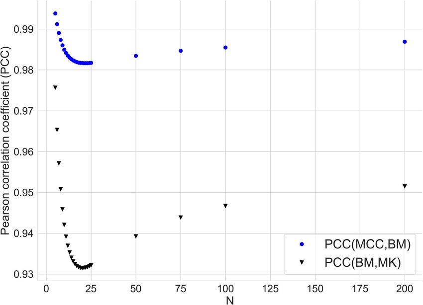
Supplementary information, and plot them in Fig. 2.
Note that, since BA and BM are analytically linked by the affine map (Eq. 15), their
mutual Pearson correlation coefficient is one, and thus we only consider BM in the cur-
rent analysis. All three series of PCC values are very high (close to 1), denoting a strong
linear relation between the three metrics. In details, PCC is slightly decreasing reach-
ing the minimum around N ≈ 25, then it increases, first quickly and then very slowly.
Further, PCC(MCC, BM) coincides with PCC(MCC, MK) for each N, even if BM and MK
Fig. 2 Pearson correlation between MCC, BM and MK as a function of number of samples NChicco et al. BioData Mining (2021) 14:13 Page 10 of 22
do not coincide: this aspect comes with no surprise, due to the symmetric form of their
expressions (Eqs. 7 and 8).
Disagreements between MCC and BM
While MCC ≈ BM ≈ MK in many instances, the most insightful cases are those
where the three metrics generate different results (Fig. 1). We present several use cases to
illustrate why outcomes may differ depending on the metric and how to interpret them.
High TPR and TNR, very low prevalence
Use case UC1. In this example we study a classification experiment with high TPR and
TNR, 0.99 and 0.95 respectively, and a very imbalanced dataset. Let us consider the
following relative confusion matrix:
TP = 9.99 × 10⁻⁴ FN = 9.99 × 10⁻⁶
relative CM1 = (29)
FP = 0.05 TN = 0.95
Assuming a sample size of 100,001, CM1 is an exemplary confusion matrix:
TP = 100 FN = 1
CM1 = (30)
FP = 5 000 TN = 94 900
MCC is 0.136, indicating that predictions from the classifier do not correlate well with
the real class. One should not make the mistake and consider the classifier to be similar
to random guessing (which always has BM=MCC=0). Objectively, the classifier is well
informed (BM = 0.94). Nevertheless, it clearly struggles to predict well for the given very
small φ.
Ultimately, MCC and BM answer different questions. BM informs us that the classi-
fier is substantially better than random guessing. Random guessing has BM = 0.0 because
it produces true positive (TP) at the same rate of false positive (FP). In UC1, this is
clearly not the case. The classifier predicts approximately 99% of reference positives as
positive and 95% of all reference negatives as negative. UC1 demonstrates that MCC
in general does not tell us if a classifier performs similarly to random guessing because
it is biased by class imbalance [52]. We are going to discuss this in greater detail later
(“Bookmaker informedness is the only metric that measures how similar a classifier is
to random guessing” subsection). In fact, the low MCC value warns us that correlation
between predicted and true class is low. This is equivalent to at least one of PPV, TPR,
TNR, NPV being low (Eq. 16), in this case PPV≈ 0.02.
A practical question would be if the classifier at hand is useful for practitioners, for
example to predict a disease. The results in Table 1 show us that applying the test consid-
erably increases our knowledge about the probability that a patient is infected. A positive
test result raises the probability to be infected by a factor of 19. Nevertheless, even those
patients that test positive are unlikely to be sick. On the other hand, those that receive a
negative test result are extremely unlikely to be sick. These findings illustrate that posi-
tive test results should not be taken at face value. Its discriminative power is not sufficient
for the tremendous class imbalance in the dataset. If this is required, a classifier with an
even higher TPR and TNR needs to be built in order to increase PPV. Yet, the present
classifier might still be helpful to identify patients which are almost certainly healthy
(receiving negative test results) from those that could profit from additional diagnostic
tests (receiving positive test results).Chicco et al. BioData Mining (2021) 14:13 Page 11 of 22
Table 1 Probability for positive data instance in UC1
Before testing φ 0.001
Testing positive PPV 0.019
Testing negative 1 – NPV 0.00001
The probability for a positive data instance, for example a patient that is truly sick, depends on the test result. While a positive test
result increases the probability substantially, it remains low. A negative test result decreases it
Misleading BA and BM, informative MCC and MK
Use case UC2. Here we analyze a use case where we have a very high number of true
positives, a high number of false negatives, and a very low number of false positives and
true negatives (Eq. 31):
TP = 8.99 × 10⁻¹ FN = 9.99 × 10⁻²
relative CM2 = (31)
FP = 9.99 × 10⁻⁶ TN = 8.99 × 10⁻⁵
If the sample size is 100,010, CM2 is an exemplary confusion matrix:
TP = 90, 000 FN = 10, 000
CM2 = (32)
FP = 1 TN = 9
We see that the classifier generates a large number of FN with respect to the number of
TN. Therefore, we can intuitively state that this classifier performed poorly: its negative
predictions are unreliable, since the NPV equals to 0.001.
Computing the confusion matrix rates, we can notice that the scores generated by the
Matthews correlation coefficient (MCC = +0.027) and the markedness (MK = 0.001)
confirm this messages: values around zero, in fact, mean inefficient classification.
The values of balanced accuracy and bookmaker informedness, however, contradict
MCC and MK. For this confusion matrix, in fact, we have BA = 0.9 and BM = 0.8, which
mean almost perfect prediction. This is a use case where BA and BM are clearly misleading:
they do not represent the low ratio of true negatives (TN= 8.99×10⁻⁵ ) over false negatives
(FN= 9.99 × 10⁻² ), that means the low negative predictive value, in this confusion matrix
(Eq. 31).
If a practitioner decided to evaluate this UC2 confusion matrix by only analyzing its
corresponding balanced accuracy and bookmaker informedness, she/he would overop-
timistically think that the classifier generated excellent predictions. The analysis of the
results achieved by MCC and MK, instead, would have kept her/him on the right track.
This conclusion closely resembles the one from UC1, because Eq. 31 would be similar
to Eq. 29 if class labels were swapped. Unlike F1 score, all the rates analyzed in this study
(MCC, BA, BM, and MK) have the advantage to be invariant to class label swapping.
Virtually uninformed classifier, slightly elevated MCC, high MK
Use case UC3. Whereas we have discussed examples of low MCC opposed to high BM
in UC1 and UC2, this use case UC3 will elaborate on the interpretation of low BM and
moderate MCC. Let us consider the following confusion matrix CM3 (Eq. 33):
TP = 0.999877792 FN = 0
relative CM3 = −4
(33)
FP = 1.11 × 10 TN = 1.11 × 10⁻⁵Chicco et al. BioData Mining (2021) 14:13 Page 12 of 22
If the sample size is 90,011, CM3 is an example of confusion matrix:
TP = 90 000 FN = 0
CM3 = (34)
FP = 10 TN = 1
Based on Eq. 33 one finds BM=0.091. The classifier at hand is only marginally better
than a “silly” rule predicting positive in all cases, which would lead to BM = 0. Both have
TPR = 1. Always predicting a positive class would lead to TNR = 0, while the presented
classifier has TNR = 0.091.
The MCC of CM3 is +0.301. While one would not consider the classifier to be good
based on this MCC, one would have a more favorable impression than based on BM.
MK is close to 1, that means almost perfect, because PPV is approximately 1 and NPV is
exactly 1. Since MCC is the geometric mean of BM and MK and MK is approximately 1,
√
MCC ≈ BM. This demonstrates that medium values of MCC cannot be interpreted in
the same way as medium values of BM.
Also, the correlation between predictions and ground truth is higher than the informed-
ness. Predictions in UC3, as measured by MK, are very reliable, not because of a well
informed classifier but rather because of the high φ.
This use case proves that MK does not reliably tell us how similar a classifier is to ran-
dom predictions. On the contrary, while the classifier is poorly informed, MK is close to
its maximum.
BM allows comparison across datasets, MCC does not
Use case UC4. The fact that MCC is dependent on φ leads to non-transferability across
datasets. This aspect needs to be considered when searching the scientific literature for
published classifiers that predict the same condition, for example a given disease.
Consider the following example. There are two publications A and B, describing two
different classifiers, for example neural networks with different architectures [56], listing
the corresponding confusion matrices and metrics (Table 2). You assume that the under-
lying datasets contain comparable samples. Based on the publications, one would like to
decide which classifier/architecture is preferable.
Comparing the Matthews correlation coefficients (Table 2), one would opt for classifier
A. Objectively, B outperforms A: MCC is only higher in publication A because the dataset
is balanced. The dataset of publication B is imbalanced, with φ = 0.05. Therefore, MCC is
low. Both TPR and TNR, the two metrics that evaluate the classifier independently of the
dataset, are higher for classifier B.
Table 2 Evaluation of two classifiers A and B on separate datasets
Classifier dataset TP FN TN FP φ TPR TNR BM MCC
(a) Relative CM
A 1 0.35 0.15 0.35 0.15 0.5 0.7 0.7 0.4 0.4
B 2 0.04 0.01 0.76 0.19 0.05 0.8 0.8 0.6 0.3
Classifier dataset TP FN TN FP φ TPR TNR BM MCC n+ n–
(b) Exemplary CM for a sample size of 200
A 1 70 30 70 30 0.5 0.7 0.7 0.4 0.4 100 100
B 2 8 2 152 38 0.05 0.8 0.8 0.6 0.3 10 190
In the literature, different publications compare classifiers for the same task on separate datasets. This poses a problem for the
comparability of metrics which are dependent on prevalenceChicco et al. BioData Mining (2021) 14:13 Page 13 of 22
Table 3 Evaluation of two classifiers A and B on the same two datasets
Classifier dataset TP FN TN FP φ TPR TNR BM MCC
(a) Relative CM
A 1 0.35 0.15 0.35 0.15 0.5 0.7 0.7 0.4 0.4
A 2 0.035 0.015 0.665 0.285 0.05 0.7 0.7 0.4 0.2
B 1 0.40 0.10 0.40 0.10 0.5 0.8 0.8 0.6 0.6
B 2 0.04 0.01 0.76 0.19 0.05 0.8 0.8 0.6 0.3
Classifier dataset TP FN TN FP φ TPR TNR BM MCC n+ n–
(b) Exemplary CM for a sample size of 200
A 1 70 30 70 30 0.5 0.7 0.7 0.4 0.4 100 100
A 2 7 3 133 57 0.05 0.7 0.7 0.4 0.2 10 190
B 1 80 20 80 20 0.5 0.8 0.8 0.6 0.6 100 100
B 2 8 2 152 38 0.05 0.8 0.8 0.6 0.3 10 190
Ideally, both classifiers are evaluated on both datasets as shown in this table. Otherwise, one should rely on metrics which are
independent of the prevalence such as BM. Matthews correlation coefficient (MCC) might be unreliable if one wants to compare
classification results across datasets
Comparing classifiers according to MCC requires that φ is identical in both datasets.
If one applied both classifiers to both datasets, it would become apparent that B outper-
forms A for either of them (Table 3). Often, reproduction is not possible (because the
datasets are not available) or tedious (because retraining the neural networks would con-
sume a lot of time and resources). Therefore, if the goal is to detect the best classifier,
we argue against comparing MCC of classifiers from different sources. In such cases, one
should rely on BM which is unbiased by class imbalance.
Interpretation of high values of multi-category metrics
When performing a binary classification, a practitioner would like to know if all four basic
rates (TPR, TNR, PPV and, NPV) are high by checking a single metric. As shown in Eq.
16, MCC generates a high score only if all four of them are high.
BM and BA are calculated based on only TPR and TNR (Eqs. 7 and 6). Therefore, it may
seem like BM is unrelated to PPV and NPV, but that is not the case, since these basic rates
can be calculated from TPR, TNR and, φ. Following our redefinition of the confusion
matrix (“Redefining confusion matrix in terms of prevalence, TPR and TNR” subsection),
we arrive at:
TPR · φ
PPV = (35)
TPR · φ + (1 − TNR) · (1 − φ)
TNR · (1 − φ)
NPV = (36)
(1 − TPR) · φ + TNR · (1 − φ)
If both TPR and TNR are high, which is the case for big values of BM and BA, at least
one of PPV and NPV must be high. One cannot know which one without knowing the
prevalence (Fig. 3). Therefore, a high BM guarantees that three of the four basic rates have
big values. If the dataset is balanced, both PPV and NPV are high if BM is high.
A high F1 score does not guarantee high TNR nor NPV because, for low φ, PPV can be
high even if TNR is low. Accuracy can be rewritten as:
accuracy = TPR · φ + TNR · (1 − φ) (37)Chicco et al. BioData Mining (2021) 14:13 Page 14 of 22
Fig. 3 Indicative example with high true positive rate (TPR) and high true negative rate (TNR). We show the
trend of the four basic rates if TPR = 0.9 and TNR = 0.8, and illustrate how positive predictive value (PPV) and
negative predictive value (NPV) depend on prevalence (φ). Bookmaker informedness (BM) equals 0.7 in this
example. At least one of PPV and NPV is high, even if φ varies. Only if φ is close to 0.6, both of them are high
Accuracy is high only if: (i) TPR and TNR are high; (ii) TPR and φ are high; or (iii) TNR
is high and φ is low. In case (i), at least one of PPV and NPV must be high as well. In case
(ii), PPV is guaranteed to be high; whereas in case (iii), NPV must be high.
It is well known that accuracy can be large although positive or negative instances are
predicted very poorly in highly imbalanced datasets [15].
Similar to Eqs. 35 and 36, TPR and TNR can be expressed in ways of PPV, NPV and, β:
PPV · β
TPR = (38)
PPV · β + (1 − NPV ) · (1 − β)
NPV · (1 − β)
TNR = (39)
(1 − PPV ) · β + NPV · (1 − β)
If MK is high, at least one of TPR and TNR must therefore be high as well. Similar to
the discussion above for BM, we cannot know which one without having identified β.
We can summarize that a high F1 score or accuracy guarantee that two of the basic rates
are high (Table 4). High BA, BM or MK guarantee that three of the basic rates are high. A
high MCC is the only multi-category metric discussed in this study that guarantees that
all four basic rates are high.
Bookmaker informedness is the only metric that measures how similar a classifier is to
random guessing
Often, papers introduce MCC with the notion that MCC = 0 signals that classifier perfor-
mance is no better than random guessing whereas a perfect classifier would have MCC =
+1. Although these statements are correct, one should avoid the misconception that MCCChicco et al. BioData Mining (2021) 14:13 Page 15 of 22
Table 4 Recap of the relationship between the multi-category metrics and the basic rates of the
confusion matrix
Scenario Basic rates condition # guaranteed high basic rates
high MCC means: high TPR, TNR, PPV, and NPV 4
high BA means: high TPR, TNR, and at least one of PPV and NPV 3
high BM means: high TPR, TNR, and at least one of PPV and NPV 3
high MK means: high PPV, NPV, and at least one of TPR and TNR 3
high F1 score means: high PPV and TPR 2
high accuracy means: high TPR and PPV, or high TNR and NPV 2
#: integer number. MCC: Matthews correlation coefficient (Eq. 5). BA: balanced accuracy (Eq. 6). BM: bookmaker informedness (Eq.
7). MK: markedness (Eq. 8). F1 score: harmonic mean of TPR and PPV (Supplementary information). Accuracy: ratio between
correctly predicted data instances and all data instances (Supplementary information). We call “basic rates” these four indicators:
TPR, TNR, PPV, and NPV
is a robust indicator of how (dis)similar a classifier is to random guessing. Only BM, and
BA, can address this topic truthfully without any distortion by φ and β.
Consider the example of three students taking an exam consisting of yes/no questions,
a scenario which is analogous to binary classification. The students randomly guess “yes”
and “no” to fill in the exam sheet because they did not prepare. The professor has the
correct solutions on their desk. While the professor is distracted, the students take the
opportunity to cheat and look up a fraction of the answers. The first one copies 25% of
the correct answers, the second one 50%, and the third one 75%.
We calculate BM, MCC and MK for the exams of the three students and display the
results in Fig. 4. BM is not at all affected by φ or β and always equals the lookup fraction.
φ corresponds to the share of questions where the correct answer would be “yes” whereas
β is the share of questions the students answered with "yes". In fact, we can define the
randomness of a classifier to be equal to 1 − BM. This will provide the correct answer
to the question: “How likely is the classifier to guess at random?”.
MCC and even more so MK can deviate from the respective lookup fraction if φ and
β are dissimilar. In this example, we know exactly that the students are 25%, 50% or 75%
informed since they have to randomly guess the rest. This fact is independent of φ and
β. Therefore, neither MCC nor MK yield a reliable estimate of how similar to random
guessing the answers of students are.
This extends to other classifiers. A value of MCC or MK close to zero should not be
considered evidence that a classifier is similar to random guessing. We note that this
deviation becomes even more extreme if φ or β approaches zero or one.
Ranking of classifiers in a real bioinformatics scenario
Similar to what we did for the study where we compared MCC with accuracy and F1
score [15], here we show a real bioinformatics scenario where the Matthews correlation
coefficient result being more informative than the other rates.
Dataset. We applied several supervised machine learning classifiers to microarray gene
expression of colon tissue collected by Alon and colleagues [57], who released it pub-
licly within the Partial Least Squares Analyses for Genomics (plsgenomics) R package
[58, 59]. This dataset comprises 2,000 gene probesets of 62 subjects; 22 of these sub-
jects are healthy controls and 40 have colon cancer (that is 35.48% negatives and 64.52%
positives) [60].Chicco et al. BioData Mining (2021) 14:13 Page 16 of 22
Fig. 4 BM, MCC and MK for classifiers with known randomness. We simulated classifiers with known amounts
of randomness. To that purpose, we generated random lists of reference classes with a given prevalence. A
fraction of those classes were copied (called lookup fraction) and used as predicted labels, the remaining
ones were generated randomly, matching a given bias. Matching the reference classes with the prediction
labels we determined bookmaker informedness, Matthews correlation coefficient and markedness (left,
center and right column respectively). The rows differ by the amount of randomness/lookup fraction
Experiment design. We used four machine learning binary classifiers to predict
patients and healthy controls in this dataset: Decision Tree [61], k-Nearest Neighbors
(k-NN) [62], Naïve Bayes [63], and Support Vector Machine with radial Gaussian
kernel [64].
Regarding Decision Trees and Naïve Bayes, we trained the classifiers on a training set
containing 80% of randomly selected data instances, and tested them on a test set con-
sisting of the remaining 20% data instances. For k-Nearest Neighbors (k-NN) and SVM,
instead, we divided the dataset into training set (60% data instances, randomly selected),
validation set (20% data instances, randomly selected), and the test set (remaining 20%
data instances). We took advantage of the validation set for the hyper-parameter opti-
mization grid search [16]: number k of neighbors for k-NN, and cost C value for the
SVM. For all the classifiers, we repeated the execution 10 times and registered the average
score for MCC, balanced accuracy, bookmaker informedness, markedness, and the four
basic rates (true positive rate, true negative rate, positive predictive value, and negative
predictive value).Chicco et al. BioData Mining (2021) 14:13 Page 17 of 22
We then ranked the results achieved on the test sets or the validation sets first based on
MCC, then based on BA, then on BM, and finally based on MK (Table 5). For the sake of
simplicity, we do not consider the uncertainty in the metrics caused by the limited sample
size and the resulting uncertainty in the rankings [53].
Results: different metric, different ranking. The four rankings we employed to report
the same results show two interesting aspects. First, the top classifier changes when we
the ranking rate changes.
In the MCC ranking, in fact, the top performing method is Decision Tree (MCC =
+0.447), while in the balanced accuracy ranking and in the bookmaker informedness
ranking the best classifier resulted being radial Naïve Bayes (BA = 0.722 and BM = 0.444).
And in the markedness ranking, even a different classifier occupied the top position:
Radial SVM with MK = 0.575. The ranks of the methods change, too: Decision Tree is
ranked first in the MCC ranking, but ranked second in the other rankings. And radial
SVM changes its rank in 3 rankings out of 4, occupying the second position in the MCC
standing, last position in the BA and BM standings, and top position in the MK stand-
ing. Only the rankings of balanced accuracy and bookmaker informedness have the same
standing, and that comes with no surprise since they contain equivalent information, as
we mentioned earlier (“BA and BM contain equivalent information” subsection).
A machine learning practitioner, at this point, could ask the question: which ranking
should I choose? As we explained earlier, in case the practitioner wants to give the same
importance to negatives and positives as well as to informedness and markedness, we
Table 5 Bioinformatics scenario: binary classification of colon tissue gene expression
Rank Method MCC BA BM MK TPR TNR PPV NPV
MCC ranking:
1 Decision Tree 0.447 0.715 0.429 0.477 0.728 0.701 0.774 0.702
2 Radial SVM 0.423 0.695 0.390 0.517 0.891 0.498 0.754 0.726
3 k-Nearest Neighbors 0.418 0.706 0.412 0.443 0.887 0.525 0.826 0.617
4 Naïve Bayes 0.408 0.722 0.444 0.375 0.778 0.667 0.875 0.500
BA ranking:
1 Naïve Bayes 0.408 0.722 0.444 0.375 0.778 0.667 0.875 0.500
2 Decision Tree 0.447 0.715 0.429 0.477 0.728 0.701 0.774 0.702
3 k-Nearest Neighbors 0.418 0.706 0.412 0.443 0.887 0.525 0.826 0.617
4 Radial SVM 0.423 0.695 0.390 0.517 0.891 0.498 0.754 0.726
BM ranking:
1 Naïve Bayes 0.408 0.722 0.444 0.375 0.778 0.667 0.875 0.500
2 Decision Tree 0.447 0.715 0.429 0.477 0.728 0.701 0.774 0.702
3 k-Nearest Neighbors 0.418 0.706 0.412 0.443 0.887 0.525 0.826 0.617
4 Radial SVM 0.423 0.695 0.390 0.517 0.891 0.498 0.754 0.726
MK ranking:
1 Radial SVM 0.423 0.695 0.390 0.517 0.891 0.498 0.754 0.726
2 Decision Tree 0.447 0.715 0.429 0.477 0.728 0.701 0.774 0.702
3 k-Nearest Neighbors 0.418 0.706 0.412 0.443 0.887 0.525 0.826 0.617
4 Naïve Bayes 0.408 0.722 0.444 0.375 0.778 0.667 0.875 0.500
Radial SVM: Support Vector Machine with radial Gaussian kernel. Positives: patients diagnosed with colon cancer. Negatives:
healthy controls. MCC: Matthews correlation coefficient(Eq. 5). BA: balanced accuracy (Eq. 6). BM: bookmaker informedness (Eq. 7).
MK: markedness (Eq. 8). TPR: true positive rate. TNR: true negative rate. PPV: positive predictive value. NPV: negative predictive
value. MCC, BM, MK value interval: [ −1, +1]. BA, TPR, TNR, PPV, NPV value interval: [ 0, 1].
Bold values represent the corresponding ranking for each metricChicco et al. BioData Mining (2021) 14:13 Page 18 of 22
suggest to focus on the ranking obtained by the MCC. A high value of MCC, in fact,
would mean that the classifier was able to correctly predict the majority of the posi-
tive data instances (TPR) and the majority of the negative data instances (TNR), and to
correctly make the majority of positive predictions (PPV) and the majority of negative
predictions (NPV). So, if the practitioner decided to base her/his study on the results of
the MCC, she/he would have more chances to have high values for the four basic rates,
than by choosing BA, BM, or MK.
Finally, we note that the differences in MCC between classifiers are small, whereas dif-
ferences of the four basic rates are relatively large. If it was desirable to have all basic rates
at a similar level, also meaning that none of them are low, Decision Tree would be the
best choice of classifiers in this scenario. SVM and k-Nearest Neighbors have high sensi-
tivity at the expense of specificity. Instead, if a high precision here was needed and a low
NPV was acceptable, the Naive Bayes classifier would be the most promising choice in
this setting. MCC does not capture these details: it only measures how well the classifiers
perform on all four basic rates together. Although MCC states that the classifiers perform
similarly well, we can see that they have both advantages and disadvantages, if compared
to each other in more detail.
Conclusions
The evaluation of binary classifications is an important step in machine learning and
statistics, and the four-category confusion matrix has emerged as one of the most power-
ful and efficient tools to perform it. To recap the meaning of a two-class confusion matrix,
researchers have introduced several statistical metrics, such as Matthews correlation
coefficient (MCC), accuracy, balanced accuracy (BA), bookmaker informedness (BM),
markedness (MK), F1 score, and others. Since the advantages of Matthews correlation
coefficient over accuracy and F1 score have been already unveiled in the past [15], in this
study we decided to compare MCC with balanced accuracy, bookmaker informedness,
and markedness, by exploring their mathematical relationships and by analyzing some
use cases.
From our analysis, we can confirm again that MCC results are generally more informa-
tive and truthful than BA, BM, and MK if the positive class and the negative class of the
dataset have the same importance in the analysis, and if correctly classifying the existing
ground truth data instances has the same importance of making correct predictions in
the analysis. Additionally, we can state that a high Matthews correlation coefficient (close
to +1) means always high values for all the four basic rates of the confusion matrix: true
positive rate (TPR), true negative rate (TNR), positive predictive value (PPV), and nega-
tive predictive value (NPV) (Table 4). The same deduction cannot be made for balanced
accuracy, bookmaker informedness, and markedness.
The situation changes if correctly classifying the existing ground truth data instances is
more important than correctly making predictions: in this case, BA and BM can be more
useful than MCC. Similarly, if making correct predictions is more relevant than correctly
identifying ground truth data instances, MK can be more informative than MCC. Instead,
if the positive data instances are more important than negative elements in a classification
(both for ground truth classification and for predictions), F1 score can be more relevant
than Matthews correlation coefficient.Chicco et al. BioData Mining (2021) 14:13 Page 19 of 22
In our analysis, we also showed two specific tasks for which bookmaker informedness
can be more useful than the other confusion matrix rates: to make a fair comparison
between two different classifiers evaluated on different datasets, and to detect the simi-
larity of a classification to random guessing. Moreover, we reported a real bioinformatics
scenario, where the usage of different rates can influence the ranking of classifiers applied
to microarray gene expression.
To conclude, as a general rule of thumb, we suggest the readership to focus on MCC
over BA, BM, and MK for any study by default, and to try to obtain a value close to +1 for
it: achieving MCC = +0.9, for example, guarantees very high F1 score, accuracy, marked-
ness, balanced accuracy, and bookmaker informedness, and even very high sensitivity,
specificity, precision, and negative predictive value. If a specific class is considered more
important (for example, predictions over ground truth classifications, or positives over
negatives), or the goal of the study is the comparison of classifiers across datasets or the
evaluation of the level of random guessing, we advise the practitioner to shift to BA, BM,
MK, or F1 score, as mentioned earlier.
In the future, we plan to compare the Matthews correlation coefficient with other met-
rics, such as Brier score [65], Cohen’s Kappa [66], K measure [67], Fowlkes-Mallows index
[68] and H-index [69].
Supplementary Information
The online version contains supplementary material available at https://doi.org/10.1186/s13040-021-00244-z.
Additional file 1: Known randomness simulation algorithm and formulas of the additional metrics.
Abbreviations
AUC: Area under the curve; BA: Balanced accuracy; BM: Bookmaker informedness; MCC: Matthews correlation coefficient;
MK: Markedness; NPV: Negative predictive value; PPV: Positive predictive value; PR: Precision-recall; ROC: Receiver
operating characteristic; TNR: True negative rate; TPR: True positive rate
Authors’ contributions
DC conceived the study; NT and GJ explored the mathematical relationships; DC and NT designed the use cases; DC
designed the bioinformatics scenario; NT investigated the random guessing aspect. All the three authors participated to
the article writing, review the article, and approved the final manuscript version.
Authors’ information
Davide Chicco (ORCID: 0000-0001-9655-7142) is with Krembil Research Institute, Toronto, Ontario, Canada.
Niklas Tötsch (ORCID: 0000-0001-7656-1160) is with Universität Duisburg-Essen, Essen, Germany.
Giuseppe Jurman (ORCID: 0000-0002-2705-5728) is with Fondazione Bruno Kessler, Trento, Italy.
Correspondence should be addressed to Davide Chicco: davidechicco@davidechicco.it
Funding
N.T. acknowledges funding from Deutsche Forschungsgemeinschaft through the project CRC1093/A7.
Availability of data and materials
Our software code is publicly available under the GNU General Public License version 3 (GPL 3.0) at: https://github.com/
niklastoe/MCC_BM_BA_MK
Ethics approval and consent to participate
Not applicable.
Consent for publication
Not applicable.
Competing interests
The authors declare they have no competing interests.Chicco et al. BioData Mining (2021) 14:13 Page 20 of 22
Author details
1 Krembil Research Institute, Toronto, Ontario, Canada. 2 Universität Duisburg-Essen, Essen, Germany. 3 Fondazione Bruno
Kessler, Trento, Italy.
Received: 1 October 2020 Accepted: 18 January 2021
References
1. Luca O. Model Selection and Error Estimation in a Nutshell. Berlin: Springer; 2020.
2. Naser MZ, Alavi A. Insights into performance fitness and error metrics for machine learning. 20201–25. arXiv preprint
arXiv:2006.00887.
3. Wei Q, Dunbrack Jr. RL. The role of balanced training and testing data sets for binary classifiers in bioinformatics.
PLoS ONE. 2013;8(7):e67863.
4. Bekkar M, Djemaa HK, Alitouche TA. Evaluation measures for models assessment over imbalanced data sets. J Inf
Eng Appl. 2013;3(10):27–38.
5. Ramola R, Jain S, Radivojac P. Estimating classification accuracy in positive-unlabeled learning: characterization and
correction strategies. In: Proceedings of Pacific Symposium on Biocomputing 2019. Singapore: World Scientific;
2019. p. 124–35.
6. Parker C. An analysis of performance measures for binary classifiers. In: Proceedings of ICDM 2011 – the 11th IEEE
International Conference on Data Mining Workshop. Vancouver: IEEE; 2011. p. 517–26.
7. Sokolova M, Lapalme G. A systematic analysis of performance measures for classification tasks. Inf Process Manag.
2009;45(4):427–37.
8. Rácz A, Bajusz D, Héberger K. Multi-level comparison of machine learning classifiers and their performance metrics.
Molecules. 2019;24(15):2811.
9. Bewick V, Cheek L, Ball J. Statistics review 13: receiver operating characteristic curves. Critic Care. 2004;8(6):508.
10. Saito T, Rehmsmeier M. The precision-recall plot is more informative than the ROC plot when evaluating binary
classifiers on imbalanced datasets. PLoS ONE. 2015;10(3):e0118432.
11. Halligan S, Altman DG, Mallett S. Disadvantages of using the area under the receiver operating characteristic curve
to assess imaging tests: a discussion and proposal for an alternative approach. Eur Radiol. 2015;25(4):932–9.
12. Wald NJ, Bestwick JP. Is the area under an ROC curve a valid measure of the performance of a screening or
diagnostic test? J Med Screen. 2014;21(1):51–56.
13. Raghavan V, Bollmann P, Jung GS. A critical investigation of recall and precision as measures of retrieval system
performance. ACM Trans Inf Syst (TOIS). 1989;7(3):205–29.
14. Cao C, Chicco D, Hoffman MM. The MCC-F1 curve: a performance evaluation technique for binary classification.
20201–17. arXiv preprint arXiv:2006.11278v1.
15. Chicco D, Jurman G. The advantages of the Matthews correlation coefficient (MCC) over F1 score and accuracy in
binary classification evaluation. BMC Genom. 2020;21(1):1–13.
16. Chicco D. Ten quick tips for machine learning in computational biology. BioData Min. 2017;10(35):1–17.
17. Matthews BW. Comparison of the predicted and observed secondary structure of T4 phage lysozyme. Biochim
Biophys Acta (BBA) Protein Struct. 1975;405(2):442–51.
18. Dinga R, Penninx BW, Veltman DJ, Schmaal L, Marquand AF. Beyond accuracy: measures for assessing machine
learning models, pitfalls and guidelines. bioRxiv. 2019;743138:1–20.
19. Handelman GS, Kok HK, Chandra RV, Razavi AH, Huang S, Brooks M, Lee MJ, Asadi H. Peering into the black box of
artificial intelligence: evaluation metrics of machine learning methods. Am J Roentgenol. 2019;212(1):38–43.
20. Jurman G, Riccadonna S, Furlanello C. A comparison of MCC and CEN error measures in multi-class prediction. PLoS
ONE. 2012;7(8):1–8.
21. Boughorbel S, Jarray F, El-Anbari M. Optimal classifier for imbalanced data using Matthews Correlation Coefficient
metric. PLoS ONE. 2017;12(6):1–17.
22. Brodersen KH, Ong CS, Stephan KE, Buhmann JM. The balanced accuracy and its posterior distribution. In:
Proceedings of ICPR 2010 – the 20th IAPR International Conference on Pattern Recognition. Istanbul: IEEE; 2010.
p. 3121–4.
23. Carrillo H, Brodersen KH, Castellanos JA. Probabilistic performance evaluation for multiclass classification using the
posterior balanced accuracy. In: Proceedings of ROBOT 2013 – the 1st Iberian Robotics Conference. Madrid:
Springer; 2014. p. 347–61.
24. Velez DR, White BC, Motsinger AA, Bush WS, Ritchie MD, Williams SM, Moore JH. A balanced accuracy function for
epistasis modeling in imbalanced datasets using multifactor dimensionality reduction. Genet Epidemiol. 2007;31(4):
306–15.
25. Hardison NE, Fanelli TJ, Dudek SM, Reif DM, Ritchie MD, Motsinger-Reif AA. A balanced accuracy fitness function
leads to robust analysis using grammatical evolution neural networks in the case of class imbalance. In: Proceedings
of GECCO 2008 – the 10th Annual Conference on Genetic and Evolutionary Computation. New York City:
Association for Computing Machinery; 2008. p. 353–354.
26. Gui J, Moore JH, Kelsey KT, Marsit CJ, Karagas MR, Andrew AS. A novel survival multifactor dimensionality
reduction method for detecting gene–gene interactions with application to bladder cancer prognosis. Hum Genet.
2011;129(1):101–10.
27. Frick A, Gingnell M, Marquand AF, Howner K, Fischer H, Kristiansson M, Williams SCR, Fredrikson M, Furmark T.
Classifying social anxiety disorder using multivoxel pattern analyses of brain function and structure. Behav Brain Res.
2014;259:330–5.
28. Ran S, Li Y, Zink D, Loo L-H. Supervised prediction of drug-induced nephrotoxicity based on interleukin-6 and-8
expression levels. BMC Bioinformatics. 2014;15(16):S16.
29. Berber T, Alpkocak A, Balci P, Dicle O. Breast mass contour segmentation algorithm in digital mammograms.
Comput Methods Prog Biomed. 2013;110(2):150–9.You can also read