Detecting Suspicious Texts Using Machine Learning Techniques - MDPI
←
→
Page content transcription
If your browser does not render page correctly, please read the page content below
applied
           sciences
Article
Detecting Suspicious Texts Using Machine
Learning Techniques
Omar Sharif 1 , Mohammed Moshiul Hoque 1, * , A. S. M. Kayes 2, * , Raza Nowrozy 2,3                  and
Iqbal H. Sarker 1
 1   Department of Computer Science and Engineering, Chittagong University of Engineering and Technology,
     Chittagong 4349, Bangladesh; omar.sharif@cuet.ac.bd (O.S.); iqbal@cuet.ac.bd (I.H.S.)
 2   Department of Computer Science and Information Technology, La Trobe University, Plenty Road, Bundoora,
     VIC 3086, Australia; r.nowrozy@latrobe.edu.au
 3   College of Engineering and Science, Victoria University, Ballarat Road, Footscray, VIC 3011, Australia
 *   Correspondence: moshiul_240@cuet.ac.bd (M.M.H.); a.kayes@latrobe.edu.au (A.S.M.K.)

 Received: 5 August 2020; Accepted: 12 September 2020; Published: 18 September 2020

 Abstract: Due to the substantial growth of internet users and its spontaneous access via electronic
 devices, the amount of electronic contents has been growing enormously in recent years through
 instant messaging, social networking posts, blogs, online portals and other digital platforms.
 Unfortunately, the misapplication of technologies has increased with this rapid growth of online
 content, which leads to the rise in suspicious activities. People misuse the web media to disseminate
 malicious activity, perform the illegal movement, abuse other people, and publicize suspicious
 contents on the web. The suspicious contents usually available in the form of text, audio, or video,
 whereas text contents have been used in most of the cases to perform suspicious activities. Thus, one of
 the most challenging issues for NLP researchers is to develop a system that can identify suspicious
 text efficiently from the specific contents. In this paper, a Machine Learning (ML)-based classification
 model is proposed (hereafter called STD) to classify Bengali text into non-suspicious and suspicious
 categories based on its original contents. A set of ML classifiers with various features has been used
 on our developed corpus, consisting of 7000 Bengali text documents where 5600 documents used for
 training and 1400 documents used for testing. The performance of the proposed system is compared
 with the human baseline and existing ML techniques. The SGD classifier ‘tf-idf’ with the combination
 of unigram and bigram features are used to achieve the highest accuracy of 84.57%.

 Keywords: natural language processing; suspicious text detection; Bengali language processing;
 machine learning; text classification; feature extraction; suspicious corpora

1. Introduction
      Due to the effortless access of the Internet, world wide web, blogs, social media, discussion
forums, and online platforms via digital gadgets have been producing a massive volume of digital
text contents in recent years. It is observed that all the contents are not genuine or authentic; instead,
some contents are faked, fabricated, forged, or even suspicious. It is very unpropitious with this rapid
growth of digital contents that the ill-usage of the Internet has also been multiplied which governs the
boost in suspicious activities [1]. Suspicious contents are increasing day by day because of ill-usage of
the Internet by a few individuals to promulgate fierceness, share illegal activities, bullying other people,
perform smishing, publicize incitement related contents, spread fake news, and so on. According to
the FBI’s Internet Crime Complaint Center (IC3) report, a total of 467,361 complaints received in the
year 2019 related to internet-facilitated criminal activity [2]. Moreover, several extremist users use

Appl. Sci. 2020, 10, 6527; doi:10.3390/app10186527                             www.mdpi.com/journal/applsci
Appl. Sci. 2020, 10, 6527                                                                             2 of 23

social media or blogs to spread suspicious and violent contents which can be considered one kind of
threat to national security [3].
       Around 245 million people are speaking in Bengali as their native tongue, which makes it the
7th most spoken language in the world [4]. However, research on Bengali Language Processing
(BLP) is currently in its initial stage, and there are no significant amount of works that have been
conducted yet like English, Arabic, Chinese, or other European languages that make Bengali a resource
constrained language [5]. As far as we are concerned, there has been no research conducted up to now
on suspicious text detection in the Bengali language. However, such systems are required to ensure
the security as well as mitigate national threats in cyber-space.
       Suspicious contents are those contents that hurt religious feelings, provoke people against
government and law enforcement agencies, motivate people to perform acts of terrorism,
perform criminal acts by phishing, smishing, and pharming, instigate a community without any
reason, and execute extortion acts [6–9]. As examples, social media has already used as a medium
of communication in Boston attack and the revolution in Egypt [10]. The suspicious contents
can be available in the form of video, audio, images, graphics, and text. However, text plays an
essential role in this context as it is the most widely used medium of communication in cyber-space.
Moreover, the semantic meaning of a conversation can be retrieved by analyzing text contents which is
difficult in other forms of content. In this work, we focus on analyzing text content and classifying the
content into suspicious or non-suspicious.
       A text could be detected as suspicious if it contained suspicious contents. It is impossible to detect
suspicious texts from the enormous amount of internet text contents manually [11]. Therefore, the automatic
detection of suspicious text contents should be developed. Responsible agencies have been demanding
some smart tool/system that can detect suspicious text automatically. It will also be helpful to identify
potential threats in the cyber-world which are communicated by text contents. Automatic detection
of suspicious text system can easily and promptly detect the fishy or threatening texts. Law and
enforcement authority can take appropriate measures immediately, which in turn helps to reduce
virtual harassment, and suspicious and criminal activities mediated through online. However, it is
a quite challenging task to classify the Bengali text contents into suspicious or non-suspicious class
due to its complex morphological structure, enormous numbers of synonym, and rich variations of
verb auxiliary with the subject, person, tense, aspect, and gender. Moreover, scarcity of resources
and lack of benchmark Bengali text dataset are the major barriers to build a suspicious text detection
system and make it more difficult to implement compared to other languages. Therefore, the research
question addressing in this paper is—“RQ: How can we effectively classify potential Bengali texts into
suspicious and non-suspicious categories?”
       To address this research question in this work, we first develop a dataset of suspicious and
non-suspicious texts considering a number of well-known Bengali data sources, such as Facebook
posts, blogs, websites, and newspapers. In order to process the textual data, we take into account
unigram, bigram, trigram features using tf-idf and a bag of words feature extraction technique.
Once the feature extraction has been done, we employ the most popular machine learning classifiers
(i.e., logistic regression, naive Bayes, random forest, decision tree, and stochastic gradient descent) to
classify whether a given text is suspicious or not. We have also performed a comparative analysis of
these machine learning models utilizing our collected datasets. The key contributions of our work are
illustrated in the following:

•     Develop a corpus containing 7000 text documents labelled as suspicious or non-suspicious.
•     Design a classifier model to classify Bengali text documents into suspicious or non-suspicious
      categories on developed corpus by exploring different feature combination.
•     Compare the performance of the proposed classifier with various machine learning techniques as
      well as the existing method.
•     Analyze the performance of the proposed classifier on different distributions of the
      developed dataset.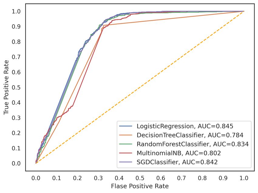
Appl. Sci. 2020, 10, 6527                                                                             3 of 23

•     Exhibits a performance comparison between human expert (i.e., baseline) and machine
      learning algorithms.

     We expect that the work presented in this paper will play a pioneering role in the development
of Bengali suspicious text detection systems. The rest of the paper organized as follows: Section 2
presents related work. In Section 3, a brief description of the development of suspicious Bengali corpus
and its several properties have explained. Section 4 explained the proposed Bengali suspicious text
document classification system and its significant constituents. Section 5 described the evaluation
techniques used to assess the performance of the proposed approach. Results of the experiments are
also presented in this section. Finally, in Section 6, we concluded the paper with a summary and
discussed the future scopes.

2. Related Work
      Suspicious contents detection is a well-studied research issue for the highly resourced languages
like Arabic, Chinese, English, and other European languages. However, no meaningful research
activities have been conducted yet to classify text with suspicious content in the BLP domain.
A machine learning-based system developed to detect promotion of terrorism by analyzing the contents
of a text. Iskandar et al. [12] have collected data from Facebook, Twitter, and numerous micro-blogging
sites to train the model. By performing a critical analysis of different algorithms, they showed that
Naïve Bayes is best suited for their work as it deals with probabilities [13]. Johnston et al. [14] proposed
a neural network-based system which can classify propaganda related to the Sunni (Sunni is a class
of Islamic believer group of Muslims: www.britannica.com/topic/Sunni) extremist users on social
media platforms. Their approach obtained 69.9% accuracy on the developed dataset. A method to
identify suspicious profiles within social media presented where normalized compression distance
was utilized to analyze text [15]. Jiang et al. [16] discusses current trends and provides future
direction to determine suspicious behaviour in various mediums of communications. The researchers
investigated the novelty of true and false news on 126,000 stories that tweeted 4.5 million times using
ML techniques [17]. An automated system explained the technique of detecting hate speech from the
Twitter data [18]. Logistic regression with regularization outperforms other algorithms by attaining
the accuracy of 90%. An intelligent system introduced to detect suspicious messages from Arabic
tweets [19]. This system yields maximum accuracy of 86.72% using SVM with a limited number of
data and class. Dinakar et al. [20] developed a corpus of YouTube comments for detecting textual
cyberbullying using a multiclass and binary classifier. A novel approach presented of detecting
Indonesian hate speech by using SVM, lexical, word unigram and tf-idf features [21]. A method
described to detect abusive content and cyberbullying from Chinese social media. Their model
achieved 95% accuracy by using LSTM and taking characteristic and behavioural features of a user [22].
Hammer [23] discussed a way of detecting violence and threat from online discussions towards
minority groups. This work considered the manually annotated sentences with bigram features of
essential words.
      Since Bengali is an under-resourced language, the amount of digitized text (related to suspicious,
fake, or instigation) is quite less. In addition to that, no benchmark dataset is available on the suspicious
text. Due to these reasons, very few research activities have carried out in this area of BLP, which are
mainly related to hate, threat, fake and abusive text detection. Ishmam et al. [24] compare machine
learning and deep learning-based model to detect hateful Bengali language. Their method achieved
70.10% accuracy by employing a gated recurrent neural network (GRNN) method on a dataset of
six classes and 5 K documents collected from numerous Facebook pages. The reason behind this poor
accuracy is the less number of training documents in each class (approximately 900). Most importantly,
they did not define the classes clearly, which is very crucial for the hateful text classification task.
Recent work explained a different machine and deep learning technique to detect abusive Bengali
comments [25]. The model acquired 82% accuracy by using RNN on 4700 Bengali text documents.
Ehsan et al. [26] discussed another approach of detecting abusive Bengali text by combining different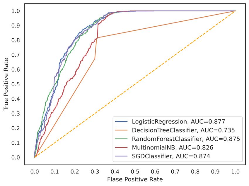
Appl. Sci. 2020, 10, 6527                                                                                      4 of 23

n-gram features and ML techniques. Their method obtained the highest accuracy for SVM with trigram
features. A method to identify malicious contents from Bengali text is presented by Islam et al. [27].
This method achieved 82.44% accuracy on an unbalanced dataset of 1965 instances by applying the
Naive Bayes algorithm. Hossain et al. [28] develop a dataset of 50 k instances to detect fake news
in Bangla. They have extensively analyzed linguistic as well as machine learning-based features.
A system demonstrated the technique to identify the threats and abusive Bengali words in social media
using SVM with linear kernel [29]. The model experimented with 5644 text documents and obtained
the maximum accuracy of 78%.
     As far as we aware, none of the remarkable research conveyed so far that focuses on detecting
suspicious Bengali text. Our previous approach used logistic regression with BoW features extraction
technique to detect suspicious Bengali text contents [30]. However, that work considered only 2000 text
documents and achieved an accuracy of 92%. In this work, our main concern is to develop the
ML-based suspicious Bengali text detection model trained on our new dataset by exploring various
n-gram features and feature extraction techniques.

3. A Novel Suspicious Bangla Text Dataset
    Up until this date, no dataset is available for identifying Suspicious Bengali Texts (SBT).
Therefore, we developed a Suspicious Bengali Text Dataset (SBTD), which is a novel annotated
corpus to serve our purpose. The following subsection explains the definition of SBT with its inherent
characteristics and details statistics of the developed SBTD.

3.1. Suspicious Text and Suspicious Text Detection
       Suspicious Text Detection (STD) system classifies a text ti eT from a set of texts T = {t1 , t2 , ..., tm }
into a class ci eC from a set of two classes C = {Cs , Cns }. The task of STD is to automatically assign ti
to ci : < ti , ci >.
       Deciding whether a Bengali text is suspicious or not is not so simple even for language experts
because of its complicated morphological structure, rich variation in sentence formation, and lack
of defining related terminology. Therefore, it is very crucial to have a clear definition of SBT for
making the task of STD smoother. In order to introduce a reasonable definition concerning the Bengali
language, several definitions of violence, incitement, suspicious, and hatred contents have analyzed.
Most of the information collected from the different social networking websites and scientific papers
summarized in Table 1.

      Table 1. Definitions of hatred, incitement and violent contents according to different social networking
      websites, organization, and scientific studies

    Source                       Definition
                                 “Contents that incite or facilitate serious violence pose credible threat to the
                                 public or personal safety, instructions to make weapons that could injure or
    Facebook
                                 kill people and threats that lead to physical harm towards private individuals
                                 or public figures” [6].
                                 “One may not promote terrorism or violent extremism, harasses or threaten
    Twitter
                                 other people, incite fury toward a particular or a class of people” [31].
                                 “Contents that incite others to promote or commit violence against
    YouTube                      individuals and groups based on religion, nationality, ethnicity, sex/gender,
                                 age, race, disability, gender identity/sexual orientation” [32].
                                 “Expression which incite, spread, promote or justify violence toward a
    Council of Europe (COE)
                                 specific individual or class of persons for a variety of reasons” [33].
                                 “Language that glorify violence and hate, incite people against groups based
    Paula et al.                 on religion, ethnic or national origin, physical appearance, gender identity
                                 or other” [7].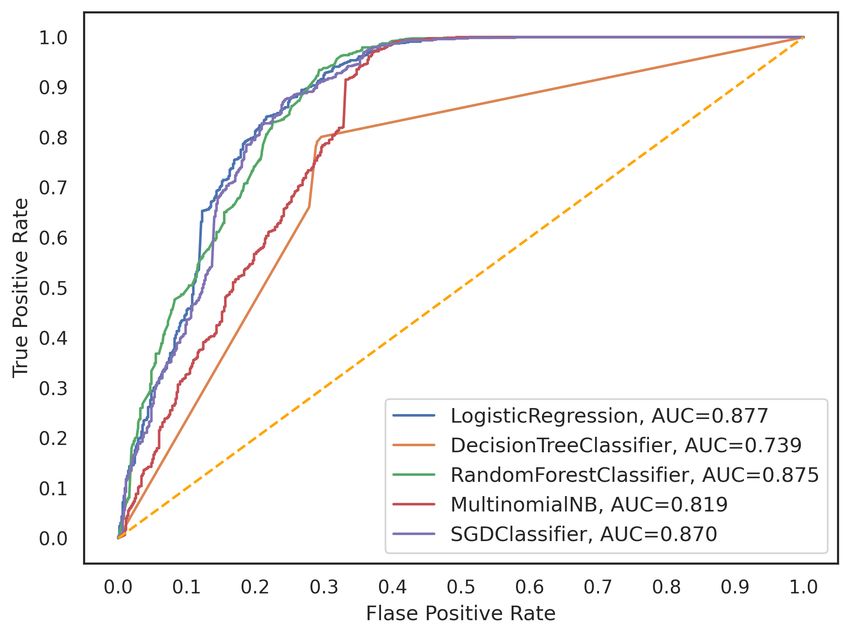
Appl. Sci. 2020, 10, 6527                                                                            5 of 23

     The majority of the quoted definitions focus on similar attributes such as incitement of violence,
promotion of hate and terrorism, and threatening a person or group of people. These definitions cover
the larger aspect of suspicious content from video, text, image, cartoon, illustrations and graphics.
Nevertheless, in this work, we concentrate on detecting suspicious content form the text contents
only. Analyzing the contents and properties of these definitions guided us to present a definition of
suspicious Bengali text as follows:

      “Suspicious Bengali texts are those texts which incite violence, encourage in terrorism,
      promote violent extremism, instigate political parties, excite people against a person
      or community based on some specific characteristics such as religious beliefs, minority,
      sexual orientation, race and physical disability.”

3.2. Development of SBT Corpora
    Bengali is the resource-constrained language due to its scarcity of digitized text contents and
unavailability of benchmark datasets. By considering the explanation of SBT and the characteristics of
suspect activity defined by the U. S. department of homeland security, we accumulated the text data
from various online sources [34]. We endorsed the same technique of developing datasets, as explained
by Das et al. [35]. Figure 1 illustrates the process of dataset development.

                                  Figure 1. Process of dataset accumulation.

     Data crowd-sourcing: Figure 2 shows the total number of texts collected from different sources in
terms of suspicious (S) and non-suspicious (NS) classes. We have crawled a total of 7115 texts among
them 3557 texts are S, and 3558 texts are NS. In the case of the suspicious class, 12.2% of source texts
collected from the website (W), 12% data collected from the Facebook comment (FC), and 10.2% from
the newspaper (N). Other sources such as Facebook posts (FP) and online blogs (OB) contributed 8.9%
and 5.4% of text data. On the other hand, a significant portion of non-suspicious source texts collected
from the newspapers (30.4%). A total of 7.8% of non-suspicious texts were collected from the OB,
5.6% from the W and 3.2% from the FC. A tiny portion of the texts was accumulated from various
sources (such as novels and articles) in both classes. As the sources of the newspapers, the three most
popular Bangladeshi newspapers are considered (such as the daily Jugantor, the daily Kaler Kontho,
and the daily Prothom Alo) for accumulating the texts.
     Data labelling: Crowd-sourced data are initially labelled by five undergraduate students of
Chittagong University of Engineering and Technology who have 8–12 months of experience in the
BLP domain. They are also doing their undergraduate thesis on BLP and attended several seminars,
webinars, and workshops on computational linguistics and NLP.
     Label verification: The expert verifies the data labels. A professor or a PhD student having more
than five years of experience or any researcher having vast experience in the BLP domain can be
considered as an expert. The final labels (Cns , Cs ) of data are decided by pursuing the process described
in Algorithm 1.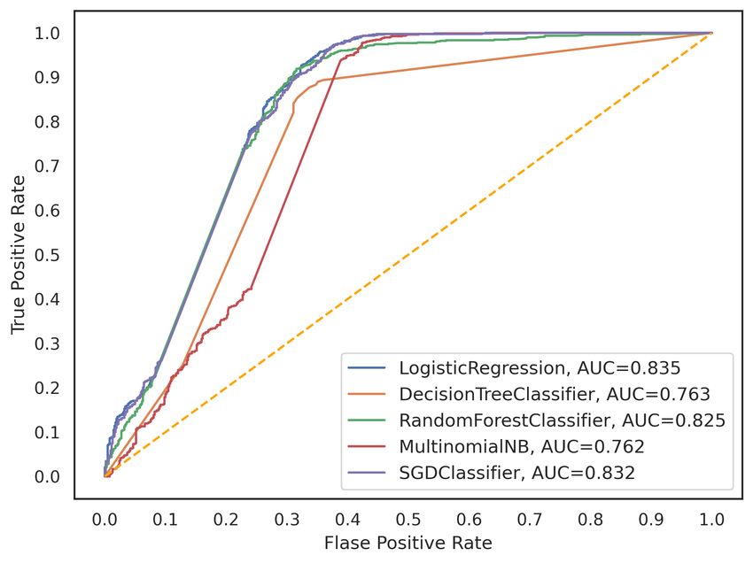
Appl. Sci. 2020, 10, 6527                                                                                  6 of 23

      Figure 2. Source texts distribution in suspicious (S) and non-suspicious (NS) categories. The acronyms
      FP, FC, W, OB, N, and M denote Facebook pages, Facebook comments, websites, online blogs,
      newspapers, and miscellaneous, respectively.

   Algorithm 1: Process of data labelling
      T ← Text Dataset;
      A ← Set of annotators;
      Final_Label ← will contain final labels;
      Initial_Label, Expert_Label;
      for ieT do
          CountS ← 0, Count NS ← 0 (initialization of suspicious and non-suspicious count);
          for a j eA do
              if a j == Cs then
                   CountS = CountS + 1;
              else
                   Count NS = Count NS + 1;
              end
          end
          Initial_Label = Count NS > CountS ? (0) : (1);
          Expert_Label = (0) || (1);
          if Initial_Label == Expert_Label then
              Final_Label [i ] = Initial_Label;
          else
              Final_Label [i ] = ‘x 0 ;
          end
          i = i + 1;
      end

      For each text in T, the annotator labels are counted. a j indicates the jth annotator label for the
ith text. If the annotator label is suspicious (Cs ), then suspicious count (CountS ) will be increased;
otherwise, the non-suspicious count (Count NS ) will increase. Majority voting [36] will decide the
initial label. If the non-suspicious count is greater than the suspicious count, then the initial label will
be non-suspicious (0); otherwise, suspicious (1). After that, the expert will label the text as either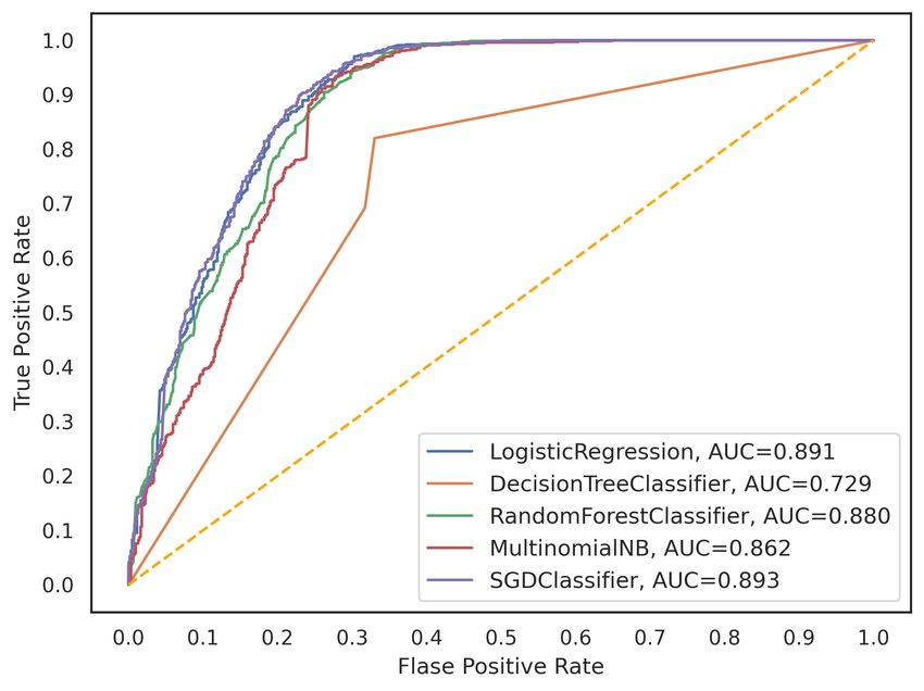
Appl. Sci. 2020, 10, 6527                                                                                          7 of 23

non-suspicious or suspicious. If the initial label matches the expert label, then it will be the final
label. When disagreement increased, the label marked with ‘x’, and the final label will be decided by a
discussion between the experts and the annotators. If they agree on a label, it will be added to SBTD;
otherwise, it will be discarded. It is noted that most of the disagreement was aroused for data of the
suspicious class. Among 900 disagreements, only 5–7% disagreement occurs for non-suspicious classes.
A small number of labels and their corresponding texts discarded from the crawled dataset due to
the disagreement between experts and annotators. Precisely, 57 for the suspicious class and 58 for the
non-suspicious class. We got 9.57% deviation on the agreement among annotators for suspicious class
and 2.34% deviation for the non-suspicious class. This deviation is calculated by averaging pairwise
deviation between annotators. Cohen’s kappa [37] between human expert and initial annotators are
88.6%, which indicates a high degree of similarity between them. Table 2 shows a sample data of our
corpus. Our data are stored in the corpus in Bangla form, but Banglish form and the English translation
is given here for better understanding.

                              Table 2. A sample text with corresponding metadata on SBTD.

                    Domain                  https://www.prothomalo.com/
                    Source                  Newspaper
                 Crawling Date              18 January 2019
                                            (Banglish form: “BPL a ek durdanto match gelo. Khulna Titans ke
                                            tin wicket a hariye dilo comilla victoria”). (English form: “A great
                     Text (ti )
                                            match was played in BPL. Comilla Victoria defeated Khulna Titans
                                            by 3 wickets”)
                   Final Label              0 (Non-Suspicious)

     Table 3 summarizes the several properties of the developed dataset. Creating SBTD was the most
challenging task for our work because all the texts demanded manual annotation. It took around ten
months of relentless work to build this SBTD. Some metadata have also been collected with the text.

                                            Table 3. Statistics of the dataset.

                            Attributes                Suspicious (Cs )            Non-Suspicious (Cns )
                   Number of documents                       3500                          3500
                        Total words                        95,629                        252,443
                    Total unique words                      18,236                        36,331
                   Avg. number of words                     27.32                         72.12
                   Maximum text length                        427                          2102
                   Minimum text length                         3                             5
                      Size (in bytes)                      688,128                       727,040

4. Proposed System
     The primary objective of this work is to develop a machine learning-based system that can
identify suspicious content in Bengali text documents. Figure 3 shows a schematic process of the
proposed system that is comprised of four major parts: preprocessing, feature extraction, training and
prediction. Input texts are processed by following several preprocessing steps explained in Section 4.1.
Feature extraction methods are employed on the processed texts to extract features. In the training
phase, exploited features are used to train the machine learning classifiers (i.e., Stochastic gradient
descent, Logistic regression, Decision tree, Random forest, and Multinomial Naïve Bayes). Finally,
the trained model will be used for classification in the prediction step. The following subsections
include the detailed explanation of the significant parts of the proposed system.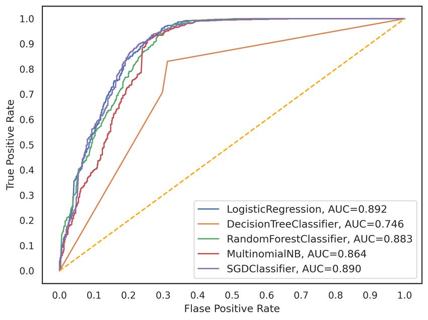
Appl. Sci. 2020, 10, 6527                                                                                     8 of 23

                    Figure 3. Schematic process of the proposed suspicious text detection system.

4.1. Preprocessing
      Preprocessing is used to transform raw data into an understandable form by removing
inconsistencies and errors. Suppose that a Bengali text document ti = (Banglish form) “Ei khulna titans
ke, tin wickete hariye dilo comilla victoria, ?...|” (English translation: Comilla Victoria defeated this
Khulna Titans by three wickets.) of the dataset T [] can be preprocessed according to the following steps:

•     Redundant characters removal: Special characters, punctuation, and numbers are removed from
      each text ti of the dataset T []. After this, ti becomes “Ei khulna titans ke tin wickete hariye dilo
      comilla victoria”.
•     Tokenization: Each text document ti is detruncated into its constituent words. A word vector of
      dimension k is obtained by tokenizing a text, ti having k words, where ti = w , w , ..., w .
     Tokenization gives a list of words of the input text such as ti = [‘Ei’, ‘khulna’, ‘titans’, ‘ke’, ‘tin’,
     ‘wickete’, ‘hariye’, ‘dilo’, ‘comilla’, ’victoria’]
•     Removal of stop words: Words that have no contribution in deciding whether a text ti is (Cs ) or
     (Cns ) is considered as unnecessary. Such words are dispelled from the document by matching
     with a list of stop words. Finally, after removing the stop words, the processed text as, ti =
     “Khulna titans ke tin wickete hariye dilo comilla victoria”. (English translation: Comilla Victoria
      defeated Khulna Titans by three wickets) will be used for training.

    With the help of the above operations, a set of processed texts is created. These texts are stored
chronologically in a dictionary in the form of array indexing A[t1 ]... A[t7000 ] with a numeric (0, 1) label.
Here, 0 and 1 represent non-suspicious and suspicious class, respectively.

4.2. Feature Extraction
     Machine learning models could not possibly learn from the texts that we have prepared.
Feature extraction performs numeric mapping on these texts to find some meaning. This work
explored the bag of words (BoW) and term frequency-inverse document frequency (tf-idf) feature
extraction techniques to extract features from the texts.
     The BoW technique uses the word frequencies as features. Here, each cell gives the count (c)
of a feature word ( f wi ) in a text document (ti ). Unwanted words may get higher weights than the
context-related words on this technique. The Tf-idf technique [38] tries to mitigate this weighting
problem by calculating the tf-idf value according to Equation (1):
                                                                                          m
                                  t f − id f ( f wi , ti ) = t f ( f wi , ti ) log                               (1)
                                                                                     |tem : f w et|

     Here, t f − id f ( f wi , ti ) indicates the tf-idf value of word f wi in text document (ti ), t f ( f wi , ti )
indicates the frequency of word f wi in text document (ti ), m means total number of text documents,
and |tem : f w et| represents the number of text document t containing word f w .
     Tf-idf value of the feature words (( f w )) puts more emphasis on the words related to the context
than other words. To find the final weighted representation of the sentences, compute the Euclidean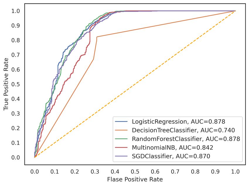
Appl. Sci. 2020, 10, 6527                                                                                                   9 of 23

norm after calculating t f − id f value of the feature words of a sentence. This normalization set high
weight on the feature words with smaller variance. Equation (2) computes the norm:
                                                              q
                                          Xnorm (i ) = Xi /       ( X1 )2 + ( X2 )2 + ... + ( Xn )2                            (2)

     Here, Xnorm (i ) is the normalized value for the feature word f wi and X1 , X2 , ..., Xn are the t f − id f
value of the feature word f w1 , f w2 , ..., f wn , respectively. Features picked out by both techniques have
been applied on the classifier.
     BoW and tf-idf feature extraction techniques are used to extract the features. Table 4 presents
the sample feature values for first five feature words ( f w1 , f w2 , f w3 , f w4 , f w5 ) of the first four text
samples (t1 , t2 , t3 , t4 ) in our dataset. Features exhibited by an array of size (m ∗ n) having m rows
and n columns. A total of 7000 text documents t1 , t2 , ..., t7000 are represented in rows while all the
feature words f w1 , f w2 , ..., f 3000 are represented in columns. In order to reduce the complexity and
computational cost, 3000 most frequent words considered as the feature words among thousands of
unique words.

              Table 4. Small fragment of extracted feature values for the first four texts of the dataset.

                                 c
                                         Technique            f w1        f w2       f w3        f w4        f w5
                       r
                                                                          Sample Feature Values
                                            BoW                1            0          4           6           2
                            t1
                                            tf-idf           0.35         0.03       0.42        0.59        0.23
                                            BoW                5            2          1           8          10
                            t2
                                            tf-idf           0.47         0.28       0.11        0.65        0.72
                                            BoW                0            1          3          12           5
                            t3
                                            tf-idf           0.04         0.11       0.22        0.75        0.44
                                            BoW                2            0          7           4           9
                            t4
                                            tf-idf           0.17         0.02       0.62        0.48        0.65

     The model extracted linguistic n-gram features of the texts. The N-gram approach is used to take
into account the sequence order in a sentence in order to make more sense from the sentences [39].
Here, ‘n’ indicates the number of consecutive words that can be treated as one gram. N-gram, as well
as a combination of n-gram features, will be applied in the proposed model.
     Table 5 shows the illustration of various n-gram features. The combination of two feature
extraction techniques and n-gram features will be applied to find the best-suited model for the
accomplishment of suspicious Bengali text detection.

          Table 5. Representation of different N-gram features for a sample Bangla text (Banglish form).

              N-grams                        “Khulna titans ke tin wickete hariye dilo comilla victoria”
              unigrams                ‘khulna’, ‘titans’, ‘ke’, ‘tin’, ‘wickete’, ‘hariye’, ‘dilo’, ‘comilla’, ‘victoria’
                                     ‘khulna titans’, ‘titans ke’, ‘ke tin’, ‘tin wickete’, ‘wickete hariye’, ‘hariye
               bigrams
                                                          dilo’, ‘dilo comilla’, ‘comilla victoria’
                                        ‘khulna titans ke’, ‘titans ke tin’, ‘ke tin wickete’, ‘tin wickete hariye’,
               trigrams
                                           ‘wickete hariye dilo’, ‘hariy dilo comilla’, ‘dilo comilla victoria’

4.3. Training
     Features that we obtained from the previous step were used to train the machine learning model
by employing different popular classification algorithms [40]. These algorithms are stochastic gradient
descent (SGD), logistic regression (LR), decision tree (DT), random forest (RF), and multinomial
naïve Bayes (MNB). We analyze these algorithms and explain their structure in our system in the
following subsections.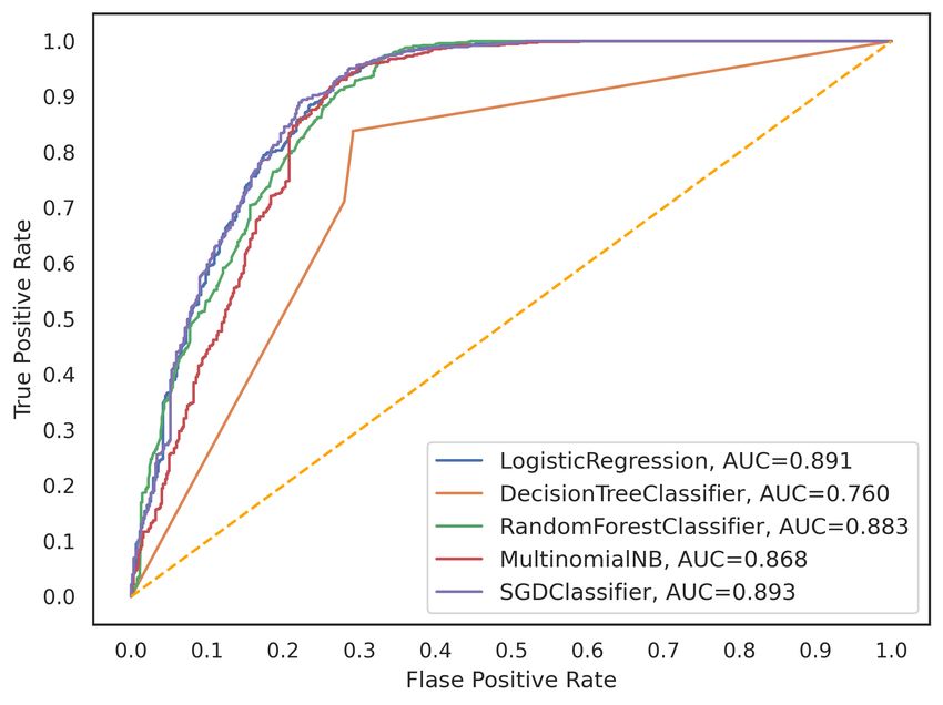
Appl. Sci. 2020, 10, 6527                                                                            10 of 23

4.3.1. Stochastic Gradient Descent
    Stochastic gradient descent (SGD) is a well-known technique used to solve ML problems [41]. It is
an optimization technique where a sample is selected randomly in each iteration instead of whole data
samples. Equations (3) and (4) represent the weight update process for gradient descent and stochastic
gradient descent at the jth iteration:
                                                          ∂J
                                          w j := w j − α                                           (3)
                                                         ∂w j
                                                                           ∂Ji
                                                 w j := w j − α                                          (4)
                                                                           ∂w j
      Here, α indicates the learning rate, J represents the cost over all training examples, and Ji is the
cost of the ith training example. It is computationally costly to calculate the sum of the gradient of the
cost function of all the samples; thus, each iteration takes a lot of time to complete [42]. To address this
issue, SGD takes one sample randomly in each iteration and calculate the gradient. Although it takes
more iteration to converge, it can reach the global minima with shorter training time. Algorithm 2
explains the process of SGD. C is the optimizer that takes θ and returns the cost and gradient. α and
theta0 represents the learning rate and the starting point of SGD, respectively.

   Algorithm 2: Process of SGD
      Function SGD(C, theta0, α, max_iter):
         θ = theta0;
         for i e max_iter do
             _ , gradient = C(θ);
             θ = θ − (α ∗ gradient);
             i++;
         end
      End Function

    We implemented the SGD classifier with ‘log’ loss function and the ‘l2’ regularization technique.
We choose a maximum number of iterations on a trial and error basis. Finally, 40 iterations are used
and samples are randomly shuffled during training.

4.3.2. Logistic Regression
     Logistic regression [43] is well suited for the binary classification problem. Equations (5)–(6)
define the logistic function that determines the output of logistic regression:

                                                                   1
                                             hθ ( x ) =                                                  (5)
                                                            1 + exp(−θ T x )

      Cost function is,
                                                                m
                                                           1
                                            C (θ ) =
                                                           m   ∑ c ( h θ ( x i ), y i )                  (6)
                                                               i −1
                                                     (
                                                         − log(1 − hθ ( x )) if y = 0
                              c ( h θ ( x ), y ) =
                                                         − log(hθ ( x ))              if y = 1

     Here, m indicates the number of training examples, hθ ( xi ) presents the hypothesis function of
the ith training example, and yi is the input label of ith training example. We used the ’l2’ norm to
penalize the classifier, and the ‘lbfgs’ optimizer is used for a maximum of 100 iterations. The default
value of the inverse of regularization strength is used with a random state 0.
Appl. Sci. 2020, 10, 6527 11 of 23
4.3.3. Decision Tree
The decision tree has two types of nodes: external and internal. External nodes represent
the decision class while internal nodes have the features essential for making classification [44].
The decision tree was evaluated in the top-down approach where homogeneous data were partitioned
into subsets. Its entropy determines the homogeneity of samples, which is calculated by the
Equation (7):
n
E(S) = ∑ pi log2 pi (7)
l =1
Here, pi is the probability of a sample in the training class, and E(S) indicates entropy of the
sample. We used entropy to determine the quality of the split. All of the features considered during
the split to choose the best split in each node. Random state 0 controls permutation of the features.
4.3.4. Random Forest
The Random Forest (RF) comprises of several decision trees which operate individually [45].
The ’Gini index’ of each branch is used to find the more likely decision branch to occur. This index
calculated by Equation (8):
c
Gini = 1 − ∑ ( p i )2 (8)
l =1
Here, c represents the total number of class and pi indicated the probability of the ith class. We
used 100 trees in the forest where the quality of split is measured by ‘gini’. Internal nodes are split if at
least two nodes are there and all the system features are considered in each node.
4.3.5. Multinomial Naïve Bayes
Multinomial Naïve Bayes (MNB) is useful to classify discrete features such as document or text
classification [46]. MNB follows multinomial distribution and uses a Bayes theorem where variables
V1 , V2 , ..., Vn of class C are conditionally independent of each other given C [47]. Equations (9) and (10)
used MNB for text classification in our dataset:
p (V | C ) p ( C )
p ( C |V ) =
p (V )
p(v1 |C ) p(v2 |C )...p(vn |C ) p(C )
p(C |(v1 , v2 , ..., vn ) = (9)
p(v1 ) p(v2 )...p(vn )
p(C ) ∏in=1 p(vi |C )
=
p(v1 ) p(v2 )...p(vn )
Here, C is the class variable and V = (v1 , v2 , ..., vn ) represents the feature vector. We assume that
features are conditionally independent. The denominator remains constant for any given input; thus,
it can be removed:
n
C = argmaxC p(C ) ∏ p ( vi |C ) (10)
i =1
Equation (10) is used to compute the probability of a given set of inputs for all possible values
of class C and pick up the output with maximum probability. Laplace smoothing used and prior
probabilities of a class are adjusted according to the data.
4.4. Prediction
In this step, the trained classifier models have been used for classification. The test set
TS = {t1 , t2 , t3 , ..., t x } has x test documents, which will be used to test the classifier model.Appl. Sci. 2020, 10, 6527 12 of 23
Predicted class (C ) is determined by using threshold ( Th ) on the predicted probability ( P) using
Equation (11):
(
Non − suspicious(Cns ) if P Th
The proposed approach classifies suspicious and non-suspicious classes as a binary classification,
so sigmoid activation function is used without tweaking the default value of Th . It ensured that both
train and test documents from the same distribution; otherwise, evaluation will not be accurate.
5. Experiments
The goal of the experiments is to analyze the performance of different machine learning classifiers
for various feature combinations. We will use several graphical and statistical measures to find
out the most suitable model that can perform well for the task of suspicious text classification.
Experimentation was carried out in an open-source Google colab platform with Python == 3.6.9
and TensorFlow == 2.2.1 [48]. Pandas == 1.0.3 data frame used for dataset preparation and training
and testing purpose, scikit-learn == 0.22.2 used. The dataset was partitioned into two independent sets:
training and testing. Data are randomly shuffled before partitioning to dispel any bias. The training
set is comprised of 80% of the total data (5600 text documents), and the testing set has 20% of the
total data (1400 text documents). In this section, we subsequently discuss the measures of evaluation
and analyze the results of experiments. In addition, we compare the proposed model with existing
techniques as well as the human baseline.
5.1. Measures of Evaluation
Various statistical and graphical measures are used to calculate the efficiency of the system. The
following terminologies have been used for evaluation purposes:
• True Positive (τp ): Texts (ti ) correctly classified as suspicious (Cs ).
• False Positive (Φ p ): Texts (ti ) incorrectly classified as suspicious (Cs ).
• True Negative (τn ): Texts (ti ) correctly classified as non-suspicious (Cns ).
• False Negative (Φn ): Texts (ti ) incorrectly classified as non-suspicious (Cns ).
• Precision: It tells how many of the ti are actually Cs among the ti that are classified as Cs .
Precision is calculated by Equation (12):
P = (τp )/(τp + Φ p ) (12)
• Recall: It gives the value of how many text documents ti classified correctly as Cs among total
suspicious texts. Recall can compute by using Equation (13):
R = (τp )/(τp + Φn ) (13)
• f 1 -score: This is a useful evaluation metric to decide which classifier to choose among several
classifiers. It is calculated by averaging precision and recall, which is done by Equation (14):
f 1 -score = (2 ∗ P ∗ R)/( P + R) (14)
As the dataset is balanced, the receiver operating characteristics (ROC) curve is therefore used for
the graphical evaluation. The trade-off between the true and false positive rate is summarized by it for
different probability thresholds.Appl. Sci. 2020, 10, 6527 13 of 23
5.2. Evaluation Results
We used scikit-learn, a popular machine learning library to implement ML classifiers.
Parameters of the classifiers tuned during experimentation. A summary of the parameters used
for each classifier is presented in Table 6.
The ‘L2’ regularization technique used with ‘lbfgs’ optimizer in logistic regression. The inverse
of the regularization strength set to 1. We select criterion as ‘entropy’ and ‘gini’ for DT and RF,
respectively, to measure the quality of a split. Both cases utilize all system features and select the best
split at each internal node of DT. We implement RF with 100 decision trees. Each node of the decision
branch is divided if it has at least two samples. In MNB, we applied adaptive smoothing and prior
probabilities adjusted according to the samples of the class. In the SGD classifier, we selected ’log’ loss
function and ‘l2’ regularization with the optimal learning rate. Samples were shuffled randomly with
a state 0 during training for a maximum of 40 iterations.
Table 6. Summary of the classifier parameters.
Classifiers Parameters
LR penalty = ‘l2 ’, C = 1.0, solver = ‘lbfgs’, max_iter = 100
criterion = ‘entropy’, splitter = ‘best’,
DT
max_features = n_features, random_state = 0
n_estimators = 100, criterion = ‘gini’,
RF
min_samples_split = 2, max_features = n_features
MNB alpha = 1.0, fit_prior = true, class_prior = none
loss = ‘log’, penalty = ‘l2 ’, learning_rate = ‘optimal’,
SGD
max_iter = 40, random_state = 0
5.2.1. Statistical Evaluation
The proposed system experimented with five different classification algorithms for BoW and tf-idf
feature extraction techniques with n-gram features. The final system evaluated with F1 = unigram,
F2 = bigram, F3 = trigram, F4 = (unigram + bigram) and F5 = (unigram + bigram + trigram) features.
Table 7 shows the comparison of performance between the classifiers for a different combination of
features. For the BoW FE technique, random forest with an F1 feature outdoes others by acquiring
83.21% accuracy. There exists a little (0.5–1)% margin among the classifiers for F1, F2, and F5 features.
All of the classifiers obtain the highest accuracy value by employing the F1 feature except DT and SGD.
DT performed well with F2 feature, whereas SGD performed for F4 features. All the classifiers showed
lower performance with F3 features. SGD achieved the highest precision value of 83.79%, and results
showed a minimum difference between precision and recall in SGD.
For the tf-idf FE technique, SGD with an F4 feature obtains the maximum accuracy of 84.57%
where the maximum precision value of 83.78% achieved for F1 features. By comparing the results of
two feature extraction techniques (i.e., BoW and tf-idf), impressive outcomes have observed in all the
evaluation parameters. Almost all the metric values have increased (2–3)% approximately by adopting
the tf-idf feature extraction technique. LR and RF obtained maximum accuracy with F1 features, MNB
and SGD gained with F4 feature and DT obtained with F2 features. Thus, in summary, the tf-idf feature
extraction and SGD classifier are well suited for our task as it outperforms the BoW technique with
other classifiers.
Figure 4 depicts the f 1 -score comparison among the classifiers for the tf-idf feature extraction
technique. We observed a tiny margin in the f 1 -score among the classifiers with F1 and F5 features.
All classifiers achieved a minimum f 1 -score for the F3 feature except DT. The DT method obtained
a minimum value of 78.74% with the F4 feature. LR and RF got the maximum value of 86.58% and
86.92%, respectively, for the F1 feature. DT obtained a maximum f 1 -score of 82.81% while MNB gotAppl. Sci. 2020, 10, 6527 14 of 23
86.57%. The results revealed that SGD with the F2 feature outperforms all other feature combinations
by obtaining an 86.97% f 1 -score.
Table 7. Performance comparison for different feature combinations where F1, F2, F3, F4, and F5
means unigram, bigram, trigram, a combination of unigram and bigram, and a combination of
unigram, bigram, and trigram features, respectively. A, P, and R denotes accuracy, precision, and
recall, respectively.
Classifier FE Features A (%) P (%) R (%)
F1 82.28 79.46 91.91
F2 81.64 77.24 94.99
BoW F3 78.07 72.18 98.58
F4 82.07 79.72 90.88
F5 82.21 79.57 91.52
LR
F1 84.00 81.14 92.81
F2 81.50 77.36 94.35
tf-idf F3 77.85 72.22 97.81
F4 83.85 80.75 93.19
F5 83.92 80.84 93.19
F1 76.00 76.78 81.51
F2 77.78 77.14 85.36
BoW F3 74.57 69.24 97.68
F4 75.57 76.67 80.61
F5 75.50 77.38 79.07
DT
F1 77.92 78.24 83.56
F2 79.57 77.85 88.44
tf-idf F3 76.14 70.69 97.56
F4 75.35 75.71 82.02
F5 76.71 76.93 83.05
F1 83.21 79.43 94.22
F2 80.50 78.68 89.08
BoW F3 76.00 70.49 97.81
F4 82.14 79.29 91.91
F5 83.20 79.82 93.45
RF
F1 83.71 78.54 97.30
F2 81.57 78.22 96.68
tf-idf F3 77.92 72.16 98.20
F4 83.21 78.14 96.91
F5 83.71 78.90 96.53
F1 81.57 79.10 90.88
F2 79.00 74.37 94.99
BoW F3 65.50 61.84 99.22
F4 81.14 77.77 92.55
F5 81.00 77.14 93.58
MNB
F1 83.78 81.29 92.04
F2 80.35 76.25 93.96
tf-idf F3 73.21 67.84 98.58
F4 83.85 80.55 93.58
F5 83.50 80.17 93.45Appl. Sci. 2020, 10, 6527 15 of 23
Table 7. Cont.
Classifier FE Features A (%) P (%) R (%)
F1 81.00 80.86 86.26
F2 81.00 76.58 94.86
BoW F3 78.21 72.31 98.58
F4 81.28 83.79 82.28
F5 78.57 81.30 79.84
SGD
F1 82.14 83.78 81.51
F2 82.00 78.06 94.09
tf-idf F3 78.92 73.54 97.04
F4 84.57 82.09 92.42
F5 83.92 81.04 93.53
Figure 4. f 1 -score comparison among different ML classifiers with F1, F2, F3, F4, and F5 features for
the tf-idf FE technique.
5.2.2. Graphical Evaluation
The ROC curve used as a measure of graphical evaluation as each class contains an equal number
of texts. Figures 5–9 exhibit the ROC curve analysis of the BoW and the tf-idf feature extraction
technique for F1, F2, F3, F4, and F5 features, respectively. For BoW with an F1 feature, logistic
regression and random forest both provide the similar AUC values of 87.8%. SGD achieved 87.0%
AUC, which increased by 2.3% by using the tf-idf FE technique. The AUC value of other algorithms
also increased by employing the tf-idf feature extraction technique.
With the F2 feature, LR obtained the maximum AUC value of 84.5%, while, for the F3 feature,
SGD achieved the maximum value. In both cases, the tf-idf feature extraction technique was used.
With tf-idf and the F4 feature, SGD beats others by getting a maximum AUC of 89.3%. The value
of all the classifiers increased except the decision tree where its value decreased by 0.06%. Results
with the F5 feature is quite similar to the F1 feature. However, LR outdoes SGD here by a margin of
0.02%. Critical analysis of results brings to the notation that the SGD classifier with the combination of
unigram and bigram feature for the tf-idf feature extraction technique achieved the highest value for
most of the evaluation parameters compared to others. The performance of the proposed classifier
(SGD) was analyzed further by varying the number of training documents to get more insight.Appl. Sci. 2020, 10, 6527 16 of 23
Figure 10 shows the accuracy versus the number of training examples graph. The analysis reveals
that the classification accuracy is increasing with the increased dataset and the tf-idf predominates the
BoW with an F2 feature.
(a) ROC curve for (BoW+F1) features (b) ROC curve for (tf-idf+F1) features
Figure 5. ROC curve analysis for the F1 feature where F1 represents the unigram feature.
(a) ROC curve for (BoW+F2) features (b) ROC curve for (tf-idf+F2) features
Figure 6. ROC curve analysis for the F2 feature where F2 represents the bigram feature.
(a) ROC curve for (BoW+F3) features (b) ROC curve for (tf-idf+F3) features
Figure 7. ROC curve analysis for the F3 feature where F3 represents the trigram feature.Appl. Sci. 2020, 10, 6527 17 of 23
(a) ROC curve for (BoW+F4) features (b) ROC curve for (tf-idf+F4) features
Figure 8. ROC curve analysis for the F4 feature where F4 represents a combination of unigram and
bigram features.
(a) ROC curve for (BoW+F5) features (b) ROC curve for (tf-idf+F5) features
Figure 9. ROC curve analysis for the F5 feature where F5 represents a combination of unigram, bigram,
and trigram features.
Figure 10. Effects of training set size on accuracy.Appl. Sci. 2020, 10, 6527 18 of 23
5.3. Human Baseline vs. ML Techniques
The performance of the classifiers compared with the human for further investigation. To eliminate
the chance of human biases in data labelling and evaluation phases, we have assigned two new experts
who manually label the testing texts into one of the predefined categories. Among 1400 test text
samples, 621 texts are from non-suspicious (Cns ) class and 779 texts are from suspicious (Cs ) class.
The accuracy of each class can be computed by the ratio between the number of correctly predicted
texts and the total number of texts of that class by using the confusion matrix. Suppose that a system
can correctly predict 730 texts among 779 suspicious texts; then, its accuracy in suspicious class will be
93.7% (730/779). As the tf-idf outperformed the BoW in the previous evaluation, we thus compared
the performance of the classifiers only for the tf-idf feature extraction technique with experts. Table 8
exhibits the summary of comparison.
Table 8. Accuracy comparison between experts and classifiers with the tf-idf FE technique.
Approach Cns Accuracy (%) Cs Accuracy (%)
Expert 1 98.71 98.58
Expert 2 99.19 98.33
LR + F1 72.94 92.81
LR + F2 65.37 94.35
LR + F3 52.81 97.81
LR + F4 72.14 93.19
LR + F5 72.30 93.19
DT + F1 70.85 83.56
DT + F2 68.43 88.44
DT + F3 42.44 97.56
DT + F4 57.69 82.02
DT + F5 68.76 83.05
RF + F1 66.66 97.30
RF + F2 67.63 96.68
RF + F3 52.49 98.20
RF + F4 66.02 96.91
RF + F5 67.63 96.53
MNB + F1 73.42 92.04
MNB + F2 63.28 93.96
MNB + F3 41.38 98.58
MNB + F4 71.65 93.58
MNB + F5 71.01 93.45
SGD + F1 72.30 81.51
SGD + F2 66.82 94.09
SGD + F3 56.19 97.04
SGD + F4 72.46 92.42
SGD + F5 70.04 93.53
The experts outperformed the ML classifiers in both classes. Experts can more accurately classify
non suspicious texts than suspicious texts. We found approximately 0.5% accuracy deviation between
experts. All of the classifiers done well on the suspicious class and performed very poorly on
the non-suspicious class. A significant difference has been observed between human baseline and
ML classifiers. All of the classifiers were able to identify suspicious texts more precisely than the
non suspicious texts. After manual analysis, we traced the reason behind this disparate behaviour.
The maximal portion of the non-suspicious texts was accumulated from the newspaper, and, on average,
each text has 72.12 words in it. ML-based classifiers did not consider the semantic meaning of a text
which is important for the classification of long texts. Thus, the system could not detect non-suspiciousAppl. Sci. 2020, 10, 6527 19 of 23
texts accurately. For this reason, the false-negative value becomes very high, which causes a drop in
the recall, and thus affects the system classification accuracy.
5.4. Comparison with Existing Techniques
As far as we aware, no meaningful research has been conducted up to now, which focused solely
on suspicious Bengali text classification. In addition to that, no benchmark dataset is available on SBT.
Therefore, the proposed work compared with the techniques has already been used on a quite similar
task. We implemented existing techniques on our developed dataset to investigate the performance
variation of the proposed approach with others. Table 9 shows the comparison in terms of accuracy for
the suspicious text classification.
Table 9. Performance comparison after employing existing techniques on our dataset.
Techniques Accuracy(%) on SBTD
SVM + BoW [19] 81.14
LR + unigram + bigram [49] 82.07
DT + tf-idf [50] 77.92
Naïve Bayes [51] 81.77
LR + BoW [30] 82.28
Our Proposed Technique 84.57
Naive Bayes [51] and SVM classifier with a BoW [19] feature extraction technique achieved a
quite similar accuracy—more than 81% accuracy on our developed dataset. LR with the combination
of unigram and bigram [49] achieved 82.07% accuracy, whereas LR with the BoW feature extraction
technique [30] also achieved similar results (82.28%). Only 77.92% accuracy was obtained for DT with
the tf-idf feature extraction technique [50], and the proposed method achieved the highest accuracy of
84.57% among existing approaches. Although the nature of the datasets is different, the result of the
comparison indicates that the proposed approach surpasses other existing techniques with the highest
accuracy on our developed dataset.
5.5. Discussion
After analyzing the experimental results, we can summarize that LR, DT, and RF do well with a
unigram feature while MNB and SGD obtained maximum accuracy with unigram and bigram feature
combination. In both cases, the tf-idf feature extraction technique is employed. Classifiers performed
poorly for trigram features. After comparing BoW and the tf-idf extraction technique, we noticed an
allusive rise for the weighted features of the texts. This increase happens because the BoW emphasizes
the most frequent words only, while the tf-idf emphasizes the context-related words more. LR, RF,
MNB, and SGD performed excellently on every feature combined with a little deviation of (0.5–0.8)%
between them. However, the performance of the decision tree is inferior compared to others due to
its limited ability to learn complex rules from texts. The AUC value is another performance measure
that indicates the model’s capability to make a distinction between classes. SGD obtained the highest
value of 0.893 AUC for the tf-idf, and LR and RF achieved the maximum AUC value of 0.878 for the
BoW feature extraction. After analysis, the reason behind the superior performance of SGD classifier is
pointed out. Here, SGD represents a linear classifier that is already proven as a well-suited model for
binary classification like ours [42]. It uses a simple approach of discriminative learning which can find
global minima more efficiently, thus resulting in better accuracy. By comparing these ML classifiers
in terms of their execution time, no significant difference has been reported. All the classifiers have
completed their execution before the 50 s mark.
Since the machine learning-based techniques mainly utilized word-level features, it is difficult
to adopt the sentence-level meanings appropriately. The system can not predict the class accurately
for this reason. Therefore, to shed light on the tendency for which text is complicated to predict inAppl. Sci. 2020, 10, 6527 20 of 23
suspicious detection, we analyze the predicted results. Consider an example, (Banglish form: “Sakib al
hasan khela pare na take bangladesh cricket team theke ber kore dewa dorkar”). (English translation:
Shakib Al Hasan cannot play, he needs to be dropped from the Bangladesh cricket team). This text may
excite the fans of Shakib Al Hasan because it conveys the disgraceful message about him. The proposed
approach should classify these texts as the suspicious class rather than the non-suspicious class.
Thus, the classification discrepancies happen due to the inability to capture the semantic relation
between words and sentence-level meanings of the texts. It is always challenging to classify such type
of text because these types of texts did not have any words that directly provoke people or pose any
threat. The proposed approach encountered a limited number of such texts during the training phase
and hence it failed to predict the class correctly. These deficiencies can be dispelled by employing
neural network-based architecture with the addition of diverse data in the existing corpus.
Although the result of the proposed SGD based model is quite reasonable compared to the
previous approaches, there are scopes to increase the overall accuracy of suspicious Bengali text
detection. Firstly, the proposed model did not consider the semantic relation between words in the
texts. For this reason, ML-based classifiers show poor accuracy for a non-suspicious class that has long
texts. The semantic relationship and corresponding machine learning rule-based model [52,53] could
also be effective depending on the data characteristics. Moreover, Deep learning techniques can be
used to find the intricate patterns from the texts that will help to comprehend the semantic relation,
but it requires a huge amount of data to effectively build the model [40,54]. Secondly, the number of
classes can be extended by introducing more sub-classes that have suspicious contents such as obscene,
religious hatred, sexually explicit, and threats. Finally, to improve the exactness of an intelligent
system, it is mandatory to train the model with a diverse and large amount of data. Therefore, a corpus
with more texts would help the system to learn more accurately and predict classes more precisely.
6. Conclusions and Future Research
In this paper, we have presented a machine learning based model to classify Bengali texts having
suspicious contents. We have used different feature extraction techniques with n-gram features in
our model. This work also computationally analyzed with a set of ML classification techniques by
taking into account the popular BoW and tf-idf feature extraction methods. Moreover, performance of
the classifiers is compared with human experts for error analysis. To serve our purpose, a dataset is
developed containing 7000 suspicious and non-suspicious text documents. After employing different
learning algorithms on this corpus, an SGD classifier and tf-idf feature extraction technique with the
combination of unigram and bigram features showed the best performance with 84.57% accuracy.
In the future, we plan to train the model with a large dataset to increase the overall performance.
Sub-domains of suspicious texts will be taken into account to make the dataset more diverse.
Furthermore, recurrent learning algorithms can be employed to capture the inherent sequential
patterns of long texts.
Author Contributions: Conceptualization, O.S. and M.M.H.; investigation, O.S., M.M.H., A.S.M.K., R.N. and
I.H.S.; methodology, O.S. and M.M.H.; software, O.S.; validation, O.S. and M.M.H.; writing—original draft
preparation, O.S.; writing—review and editing, M.M.H., A.S.M.K., R.N. and I.H.S. All authors have read and
agreed to the published version of the manuscript.
Funding: This research received no external funding.
Conflicts of Interest: The authors declare no conflict of interest.
References
1. Khangura, A.S.; Dhaliwal, M.S.; Sehgal, M. Identification of Suspicious Activities in Chat Logs using
Support Vector Machine and Optimization with Genetic Algorithm. Int. J. Res. Appl. Sci. Eng. Technol.
2017, 5, 145–153.
2. Internet Crime Complaint Center (U.S.), United States, F.B.O.I. 2019 Internet Crime Report. 2020. pp. 1–28.
Available online: https://www.hsdl.org/?view&did=833980 (accessed on 22 May 2020)You can also read