Object-Based Land Cover Classification of Cork Oak Woodlands using UAV Imagery and Orfeo ToolBox
←
→
Page content transcription
If your browser does not render page correctly, please read the page content below
remote sensing
Article
Object-Based Land Cover Classification of Cork Oak
Woodlands using UAV Imagery and Orfeo ToolBox
Giandomenico De Luca 1 , João M. N. Silva 2, * , Sofia Cerasoli 2 , João Araújo 3 ,
José Campos 3 , Salvatore Di Fazio 1 and Giuseppe Modica 1, *
 1    Dipartimento di Agraria, Università degli Studi Mediterranea di Reggio Calabria, Località Feo di Vito,
      I-89122 Reggio Calabria, Italy; delucagiandomenico@gmail.com (G.D.L.); salvatore.difazio@unirc.it (S.D.F.)
 2    Forest Research Centre, School of Agriculture, University of Lisbon, Tapada da Ajuda, 1349-017 Lisbon,
      Portugal; sofiac@isa.ulisboa.pt
 3    Spin.Works S.A., Avenida da Igreja 42, 6º, 1700-239 Lisboa, Portugal; joao.araujo@spinworks.pt (J.A.);
      jose.campos@spinworks.pt (J.C.)
 *    Correspondence: joaosilva@isa.ulisboa.pt (J.M.N.S.); giuseppe.modica@unirc.it (G.M.)

 Received: 18 February 2019; Accepted: 21 May 2019; Published: 24 May 2019

 Abstract: This paper investigates the reliability of free and open-source algorithms used in the
 geographical object-based image classification (GEOBIA) of very high resolution (VHR) imagery
 surveyed by unmanned aerial vehicles (UAVs). UAV surveys were carried out in a cork oak woodland
 located in central Portugal at two different periods of the year (spring and summer). Segmentation
 and classification algorithms were implemented in the Orfeo ToolBox (OTB) configured in the QGIS
 environment for the GEOBIA process. Image segmentation was carried out using the Large-Scale
 Mean-Shift (LSMS) algorithm, while classification was performed by the means of two supervised
 classifiers, random forest (RF) and support vector machines (SVM), both of which are based on
 a machine learning approach. The original, informative content of the surveyed imagery, consisting
 of three radiometric bands (red, green, and NIR), was combined to obtain the normalized difference
 vegetation index (NDVI) and the digital surface model (DSM). The adopted methodology resulted in
 a classification with higher accuracy that is suitable for a structurally complex Mediterranean forest
 ecosystem such as cork oak woodlands, which are characterized by the presence of shrubs and herbs
 in the understory as well as tree shadows. To improve segmentation, which significantly affects the
 subsequent classification phase, several tests were performed using different values of the range
 radius and minimum region size parameters. Moreover, the consistent selection of training polygons
 proved to be critical to improving the results of both the RF and SVM classifiers. For both spring
 and summer imagery, the validation of the obtained results shows a very high accuracy level for
 both the SVM and RF classifiers, with kappa coefficient values ranging from 0.928 to 0.973 for RF
 and from 0.847 to 0.935 for SVM. Furthermore, the land cover class with the highest accuracy for
 both classifiers and for both flights was cork oak, which occupies the largest part of the study area.
 This study shows the reliability of fixed-wing UAV imagery for forest monitoring. The study also
 evidences the importance of planning UAV flights at solar noon to significantly reduce the shadows
 of trees in the obtained imagery, which is critical for classifying open forest ecosystems such as cork
 oak woodlands.

 Keywords: Geographic Object-Based Image Analysis (GEOBIA); Land cover classification; Unmanned
 Aerial Vehicles (UAVs); Orfeo ToolBox (OTB); cork oak woodlands; machine learning algorithms;
 Random Forest (RF); Support Vector Machines (SVM); Spectral separability; Accuracy assessment

Remote Sens. 2019, 11, 1238; doi:10.3390/rs11101238                          www.mdpi.com/journal/remotesensing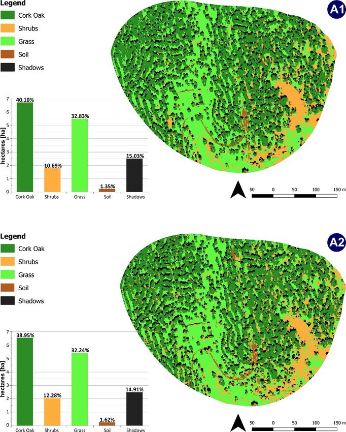
Remote Sens. 2019, 11, 1238                                                                          2 of 22

1. Introduction
       Cork oak woodlands characterize forested Mediterranean landscapes, and their ecological and
economic values are largely recognized, although not adequately valorized [1]. This ecosystem covers
about 2.2 million hectares across the globe, but the most extensive groves are located on the Atlantic
coast of the Iberian Peninsula, to the extent that Portugal and Spain produce 75% of the world’s
cork [2]. Cork is the sixth-most important non-wood forest product globally, and it is used to produce
wine stoppers and a wide variety of other products, including flooring components, insulation and
industrial materials, and traditional crafts. The most frequent landscape in the Mediterranean region is
characterized by open woodland systems in which scattered mature trees coexist with an understory
composed of grassland for livestock or cereal crops and shrubs. The ecosystem has high conservation
value and provides a broad range of goods and services besides cork [2]. It is important to increase the
knowledge and skills that enable the use of the most innovative technologies to monitor these forest
ecosystems in the support of forest management.
       The use of unmanned aerial vehicles (UAVs) or UA systems (UASs) in forest and environmental
monitoring [3–15] is currently in an expansion phase, encouraged by the constant development of
new models and sensors [3,16,17]. Detailed reviews focusing on the use of UAVs in agro-forestry
monitoring, inventorying, and mapping are provided by Tang and Shao [16], Pádua et al. [3], and
Torresan et al. [18]. Additionally, the short time required for launching a UAV mission makes it possible
to perform high-intensity surveys in a timely manner [16,19,20], thus granting forest practices with
more precision and efficiency while opening up new perspectives in forest parameter evaluation.
Therefore, UAVs are particularly suitable for multi-temporal analysis of small- and medium-sized land
parcels and complex ecosystems, for which frequent surveys are required [17].
       There is a large diversity of UAV applications, mainly as a result of the variety of available
sensors [21]. The most common sensors assembled on UAVs are passive sensors, which include classic
RGB (red, green, blue) cameras, NIR (near-infrared), SWIR (short-wave infrared), MIR (mid-infrared),
TIR (thermal infrared), and their combinations in multispectral (MS) and hyperspectral (HS) cameras
and active sensors such as RADAR (radio detection and ranging) and LiDAR (laser imaging detection
and ranging) [3,16]. An increasingly common agro-forestry application that uses multispectral images
acquired from sensors assembled on UAVs is land cover classification [18,22].
       Until a decade ago, most of the classification methods for agro-forestry environments were based
on the statistical analysis of each separate pixel (i.e., pixel-based method), and performed well when
applied to satellite imagery covering large areas [23–25]. The recent emergence of very high resolution
(VHR) images, which are becoming increasingly available and cheaper to acquire, has introduced
a new set of possibilities for classifying land cover types at finer levels of spatial detail. Indeed, VHR
images frequently show high intra-class spectral variability [19,20,26]. On the other hand, the higher
spatial resolution of these images enhances the ability to focus on an image’s structure and background
information, which describe the association between the values of adjacent pixels. With this approach,
spectral information and image classification are largely improved [27].
       Recently, object-based image analysis (OBIA) has emerged as a new paradigm for managing
spectral variability, and it has replaced the pixel-based approach [27,28]. OBIA works with groups of
homogeneous and contiguous pixels [19] (i.e., geographical objects, also known as segments) as base
units to perform a classification, so it differs from the classic pixel-oriented methods that classify each
pixel separately; thus, the segmentation approach reduces the intra-class spectral variability caused
by crown textures, gaps, and shadows [19,27,28]. OBIA includes two main steps: (i) identification,
grouping, and extraction of significant homogeneous objects from the input imagery (i.e., segmentation);
(ii) labeling and assigning each segment to the target cover class (classification) [19,20,28].
       More recently, considering that OBIA techniques are applied in many research fields, when
referring to a geospatial context, the use of GEOBIA (geographic OBIA) [27,29,30] has become the
preferred method. Moreover, GEOBIA should be considered as a sub-discipline of GIScience, which
is devoted to obtaining geographic information from RS imagery analysis [27,29,30]. GEOBIA has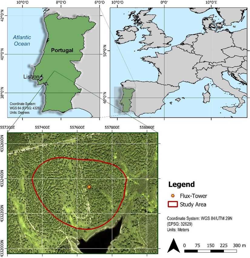
Remote Sens. 2019, 11, 1238                                                                               3 of 22

proven to be successful and often superior to the traditional pixel-based method for the analysis of
very high resolution UAV data, which exhibits a large amount of shadow, low spectral information,
and a low signal-to-noise ratio [6,19,20,26].
      The availability of hundreds of spectral, spatial, and contextual features for each image object can
make the determination of optimal features a time-consuming and subjective process [20]. Therefore,
high radiometric and geometric resolution data require the simultaneous use of more advanced and
improved computer software and hardware solutions [26]. Several works dealing with the classification
of forest ecosystems or forest tree species by coupling GEOBIA and UAV imagery can be found in the
literature [4,15,16,22,31]. Franklin and Ahmed [31] reported the difficulty in performing an accurate
tree crown reconstruction, characterizing fine-scale heterogeneity or texture, and achieving operational
species-level classification accuracy with low or limited radiometric control. Deciduous tree species
are typically more difficult to segment into coherent tree crowns than evergreens [31] and tend to be
classified with lower accuracies [32].
      In terms of using GEOBIA algorithms, most studies are implemented by means of proprietary
software (e.g., [4,6,11,15,19,31]). Considering their cost, especially in an operational context, it can
be argued that only a relatively restricted group of operators can use them. Nowadays, several free
and open-source software packages for geospatial (FOSS4G) analysis with GEOBIA algorithms are
available, thus making their use accessible to a larger number of end users [20]. Among others, a very
promising FOSS4G package equipped with GEOBIA algorithms is Orfeo ToolBox (OTB), developed
by the French Centre National d’Etudes Spatiales (CNES). OTB can be operated either autonomously
or through a second open-source software (i.e., QGIS), used as a graphical interface that enables
a graphical analysis of data processing in real time [33,34].
      This work was conducted in the framework of a wider project aiming to derive a methodology for
monitoring the gross primary productivity (GPP) of Mediterranean cork oak (Quercus suber L.) woodland
by integrating spectral data and biophysical modeling. The spatial partition of the ecosystem into different
coexisting vegetation layers (trees, shrubs, and grass), which is the task encompassed by this study,
is essential to the fulfillment of the objective of the overarching project. The main objective of this work
was to develop a supervised classification procedure of the three vegetation layers in a Mediterranean
cork oak woodland by applying a GEOBIA workflow to VHR UAV imagery. In order to optimize the
procedure, two different algorithms were compared: support vector machine (SVM) and random forest
(RF). In addition, data from two contrasting surveying periods—spring and summer—were also compared
in order to assess the effect of the composition of different layers (i.e., no living grass in the summer period)
on the classification accuracy. In order to increase the processing quality, we tested a methodology based
on the combination of spectral and semantic information to improve the classification procedure through
the combined use of three informative layers: R-G-NIR mosaics, NDVI (normalized difference vegetation
index), and DSM (digital surface model).
      The paper is organized as follows. Section 2 provides details about the study area and the dataset,
and gives a general description of OTB. Section 3 deals with methodological issues by explaining
preprocessing, segmentation, classification methods and tools, and the performed accuracy analyses.
In Section 4, the obtained results are shown, and they are discussed in Section 5. Section 6 summarizes
the results and highlights the limitations of the present research, open questions, and suggested future
research directions.

2. Materials

2.1. Study Area
     The study area is located in Central Portugal (39º08’ N; 08º19’ W) and covered by a Mediterranean
cork oak woodland (Figure 1). The climate is typically Mediterranean with hot and dry summers, while
most of the precipitation is concentrated between autumn and early spring (from October to April).
Quercus suber is the only tree species present, and the understory is composed of a mixture of shrubs and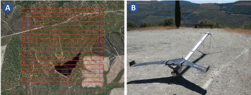
to the fluxes [37].

2.2. Dataset

2.2.1 Data Acquisition
  Remote Sens. 2019, 11, 1238                                                                                      4 of 22
     We used a fixed-wing UAV (SpinWorks S20; Figure 2) with a wingspan of 1.8 m and a modified
RGB camera with a radiometric resolution of 8 bit per channel in which the blue channel was replaced
byherbaceous    species [35].
   an NIR channel.            The shrubby
                        The main           layer is composed
                                    characteristics           primarily
                                                     of the S20         of two species,
                                                                are summarized          Cistus1,salvifolius
                                                                                   in Table                 and
                                                                                                  while further
  Ulex airensis, while the herbaceous layer is dominated by C3 species, mainly grasses and legumes. The site
descriptive details can be found in Soares et al. [38]. Flight planning (Figure 2) was carried out using
  is a permanent research infrastructure where carbon, water, and energy are regularly measured by eddy
the ground station software integrated with the S20 system that was developed by the SpinWorks
  covariance [36]. The study area is delimited by the 70% isoline of the flux tower footprint—an estimate
company [38].
  of the extent and position of the surface contributing to the fluxes [37].

        Figure 1. The top figure shows the location of the study area in Central Portugal. Below, the location of
     Figure    1. The
        the flux      top
                  tower   figure
                        and       shows
                             the 70%      theoflocation
                                     isoline             of theclimatology
                                                 the footprint   study arearepresenting
                                                                            in Central Portugal.
                                                                                        the study Below,
                                                                                                  area are the location
                                                                                                            identified
     of in
         thea UAV
              flux tower   and the 70% isoline of the footprint climatology representing the study area are
                    orthomosaic.
     identified in a UAV orthomosaic.
  2.2. Dataset

  2.2.1. Data Acquisition
        We used a fixed-wing UAV (SpinWorks S20; Figure 2) with a wingspan of 1.8 m and a modified
  RGB camera with a radiometric resolution of 8 bit per channel in which the blue channel was replaced by
  an NIR channel. The main characteristics of the S20 are summarized in Table 1, while further descriptive
  details can be found in Soares et al. [38]. Flight planning (Figure 2) was carried out using the ground
  station software integrated with the S20 system that was developed by the SpinWorks company [38].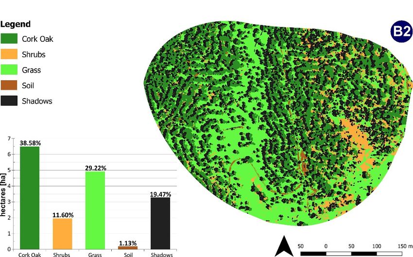
Remote Sens. 2019, 11, 1238                                                                                  5 of 22
Remote Sens. 2019, 11, x FOR PEER REVIEW                                                                              5 of 22

     Figure
          Figure  2. Flight
            2. Flight  planplan (red)
                            (red) andand  flight
                                      flight     path
                                              path    (yellow)(A).
                                                    (yellow)   (A). The
                                                                    The fixed-wing
                                                                        fixed-wingUAV
                                                                                   UAVS20 before
                                                                                        S20      take-off
                                                                                            before        (B). (B).
                                                                                                    take-off
           Table 1. Technical characteristics of the S20 unmanned aerial vehicle (UAV) and the onboard camera [38],
2.2.2 Flight
          andData  Processing
              features of the two and
                                  flightsOutputs
                                          (spring and summer).
     Photogrammetric and image processing                 proceduresofwere
                                              Technical Characteristics    S20 carried out and are synthetically
depicted in Maximum
              the workflow         (Figure 3). In this procedure, each image
                          take-off weight                                             2.0 kg
                                                                                                taken in-flight has the
geographical Maximum
              position weight
                          and elevation      logged   using
                                  of the payload (sensors)   the  navigation     system
                                                                                      0.4 kgand   the onboard computer.
              Maximum flight
With this information,           autonomy
                           the raw                                                      2h
                                       dataset is processed using a structure-from-motion                (SFM) technique
              Cruising speed                                                        60 km h−1
during which the identification of common features in overlapping images is carried out.
              Maximum operating range drone- pilot station                            20 km
Subsequently,productivity
                 a 3D point        cloud
                             (hectares      is generated from which a digital
                                       per hour)                                    200 ha h−1surface model (DSM) is
interpolated, Bands
              which in turn is used to orthorectify each image. Finally,                all ofNIR
                                                                                Red, Green,    these images are stitched
              Pixel resolution                                                       12.1 Mpx
together in an orthomosaic. Two orthomosaics were derived from two flights that were carried out
              Size of the sensor                                                  7.6 × 5.7 mm
in different seasons    of 2017: spring (5 April at 13:00) and summer
              Field of view                                                             (13degrees
                                                                              73.7 × 53.1     July at 11:00) (Table A1).
Moreover, eachFocusorthomosaic was radiometrically corrected in post-processing       24 mm            using a calibrated
              Ground   sample   distance (GSD)                       5  cm pixel−1 at 100 m of flight height
reflectance panel imaged before and after each of the flights. The use of the same scene in two
different periods allowed for testing the       Features of the twoalgorithm’s
                                                  classification    flights         capacity to take into account the
              Covered area                                                         100 hectares
differences caused     by variation in the phenological status as it changed
              Flight height                                                           100 m throughout the various
biological cycles of the
              Sidelap  andmain    plant species. The resultant mosaics have
                            overlap                                               60%an   extension
                                                                                        and  90%       of 100 ha (a square
              N ◦ of photos                                                            1500
of 1000 × 1000 m) and a resampled GSD (ground sample distance) of 10 cm.
                 Duration of flights                                    41 min (spring), 28 min (summer)

         Table 1. Technical characteristics of the S20 unmanned aerial vehicle (UAV) and the onboard
     2.2.2. Flight Data Processing
                        camera [38],and
                                     andOutputs
                                         features of the two flights (spring and summer).
          Photogrammetric and image processing procedures were carried out and are synthetically depicted
                                          Technical characteristics of S20
     in the workflow (Figure 3). In this procedure, each image taken in-flight has the geographical position and
    Maximum      take-off
     elevation logged       weight
                        using  the navigation system and the onboard computer. With this  2.0 information,
                                                                                               kg           the raw
    Maximum      weight of
     dataset is processed      the apayload
                            using             (sensors)
                                     structure-from-motion   (SFM) technique during which 0.4 kg
                                                                                               the identification of
    Maximum      flight autonomy
     common features      in overlapping images is carried out. Subsequently, a 3D point    2 hcloud is generated
    Cruising
     from whichspeed
                   a digital surface model (DSM) is interpolated, which in turn is used 60 km  tohorthorectify
                                                                                                   -1          each
     image.   Finally, all of these  images  are
    Maximum operating range drone- pilot station stitched together in an orthomosaic.    Two
                                                                                          20 km orthomosaics   were
     derived from (hectares
    productivity    two flightsper
                                 thathour)
                                      were carried out in different seasons of 2017: spring  (5 April
                                                                                        200 ha   h-1 at 13:00) and
     summer
    Bands      (13 July  at 11:00)  (Table A1).  Moreover,  each orthomosaic   was Red, Green, NIRcorrected in
                                                                                    radiometrically
     post-processing using a calibrated reflectance panel imaged before and after each of the flights. The use
    Pixel  resolution                                                                   12.1 Mpx
     of the same scene in two different periods allowed for testing the classification algorithm’s capacity to
    Size of the sensor                                                                7.6 × 5.7 mm
     take into account the differences caused by variation in the phenological status as it changed throughout
    Field of view                                                                 73.7 × 53.1 degrees
     the various biological cycles of the main plant species. The resultant mosaics have an extension of 100 ha
    Focus
     (a square of 1000 × 1000 m) and a resampled GSD (ground sample distance) of24        10 mm
                                                                                             cm.
    Ground sample distance (GSD)                                    5 cm pixel-1 at 100 m of flight height
                                             Features of the two flights
    Covered area                                                                 100 hectares
    Flight height                                                                    100 m
    Sidelap and overlap                                                         60% and 90%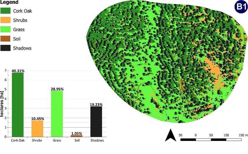
Remote Sens. 2019, 11, 1238                                                                                 6 of 22
Remote Sens. 2019, 11, x FOR PEER REVIEW                                                                             7 of 22

         Figure
     Figure        Workflow ofof
             3. 3.Workflow     thethe
                                   preprocessing, segmentation,
                                        preprocessing,           classification,
                                                           segmentation,         and validationand
                                                                              classification,   steps validation
                                                                                                      implementedsteps
         to derive an object-based land cover map   for cork oak woodlands     from UAV   imagery.
     implemented to derive an object-based land cover map for cork oak woodlands from UAV imagery.

3.3. Segmentation
     Segmentation is the first phase of the object-oriented classification procedure, and its result is a
vector file in which every polygon represents an object. Original images are subdivided into a set of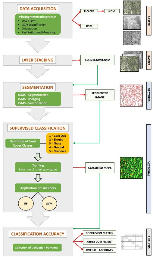
Remote Sens. 2019, 11, 1238                                                                             7 of 22

2.3. ORFEO ToolBox (OTB)
     OTB is an open-source project for processing remotely sensed imagery, developed in France
by CNES (www.orfeo-toolbox.org, accessed 10 April 2019) [39]. It is a toolkit of libraries for image
analysis and is freely accessible and manageable by other open-source software packages as well as
command-line [33,34,40]. The algorithms implemented in OTB were applied in this work through the
QGIS software (www.qgis.org, accessed 10 April 2019). The OTB version used was 6.4.0; it interfaced with
QGIS 2.18 Las Palmas, which was installed on an outdated workstation (Table A2). This is an important
detail that highlights the fluidity of OTB because it works even with underperforming hardware.
In OTB, the algorithms used in the phase of image object analysis were Large-Scale Mean-Shift (LSMS)
segmentation for the image segmentation, and SVM and RF for the object-based supervised classification.

3. Methods
     The implemented workflow can be simplified into four main steps: preprocessing, segmentation,
classification, and accuracy assessments (Figure 3).

3.1. Preprocessing
      For both the spring and summer flights, a DSM with a GSD of 10 cm was derived for its usefulness
in further classification stages since trees, shrubs, and grass have very different heights. For every
informative layer used in the next stage of classification, and therefore for every input layer, a linear band
stretching (rescale) to a range at 8 bits, from 0 (minimum) to 255 (maximum), was performed. The aim of
this process, as described in Immitzer et al. [41], was to normalize each band to a common range of values
in order to reduce the effect of potential outliers on the segmentation. Subsequently, for both raster files
(spring and summer) containing the R-G-NIR bands, a layer stacking process was performed by merging
NDVI and DSM data to obtain two final five-band orthomosaics. This step was necessary because OTB
segmentation procedure requires a single raster image as input data. Successively, a window of the
original scene was made so that only a smaller area of interest, corresponding to the footprint of the flux
tower, was classified (approximately 16.85 ha).

3.2. Spectral Separability
     In order to measure the separability of the NDVI and the DSM layers of different types of vegetation
present in the study area (cork oak, shrubs, and grass) and, consequently, their importance for the
classification provided by the original spectral bands (R-G-NIR), we implemented the M-statistic,
defined originally by Kaufman and Remer and modified as follows:

                                                     µ1 − µ2
                                              M=                                                           (1)
                                                     (σ1 + σ2)

where µ1 is the mean value for class 1, µ2 is the mean value for class 2, σ1 is the standard deviation for
class 1, and σ1 is the standard deviation for class 2. M-statistic expresses the difference in µ (the signal)
normalized by the sum of their σ (that can be interpreted as the noise) (i.e., the separation between
two samples by class distribution). Larger σ values lead to more overlap of the two considered bands,
and therefore to less separability. If M < 1, classes significantly overlap and the ability to separate
(i.e., to discriminate) the regions is poor, while if M > 1, class means are well separated and the regions
are relatively easy to discriminate.

3.3. Segmentation
     Segmentation is the first phase of the object-oriented classification procedure, and its result is
a vector file in which every polygon represents an object. Original images are subdivided into a set
of objects (or segments) that are spatially adjacent, composed of a set of pixels with homogeneity or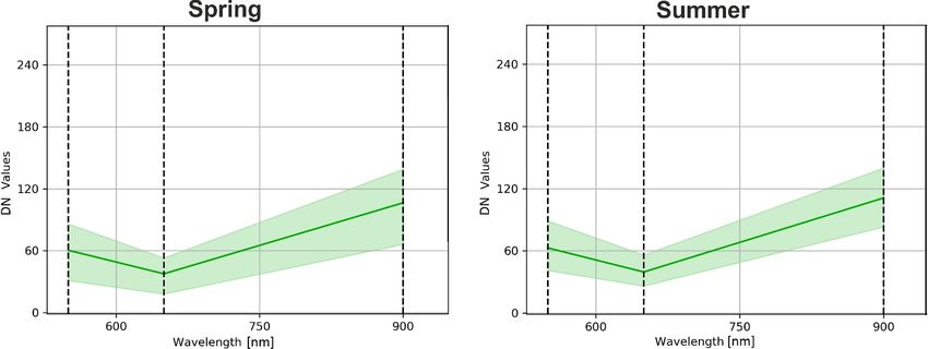
Remote Sens. 2019, 11, 1238                                                                            8 of 22

semantic meaning, and collectively cover the whole image. The shape of every notable object should
be ideally represented by one real object in the image [19,27]. Segmentation focuses not only on the
radiometric information of the pixels, but also on the semantic properties of each segment, on the
image structure, and on other background information (color, intensity, texture, weft, shape, context,
dimensional relations, and position) whose values describe the association between adjacent pixels.
     The Large-Scale Mean-Shift (LSMS)-segmentation algorithm is a non-parametric and iterative clustering
method that was introduced in 1975 by Fukunaga and Hostetler [42]. It enables the performance of tile-wise
segmentation of large VHR imagery, and the result is an artifact-free vector file in which each polygon
corresponds to a segmented image containing the radiometric mean and variance of each band [33,34].
This method allows for the optimal use of the memory and processors, and was designed specifically for
large-sized VHR images [42]. The OTB LSMS-segmentation procedure is composed of four successive
steps [33,34]:

1.    LSMS-smoothing;
2.    LSMS-segmentation;
3.    LSMS-merging;
4.    LSMS-vectorization.

      In the first phase, we tested the reliability of LSMS-smoothing in the segmentation process by
adopting different values of the spatial radius (i.e., the maximum distance to build the neighborhood
from averaging the analyzed pixels [35]). Starting from the default value of the spatial radius (5),
we tested the following values: 5–10, 15, 20, and 30. However, considering that LSMS-smoothing
did not improve the results of the segmentation process and is an optional step, we omitted it. Thus,
we started from the second step (LSMS-segmentation).
      For this step, the literature was reviewed to make an informed choice of the values of the different
parameters. However, all examined publications focus on the urban field and the use of satellite
imagery. This highlights the lack of previous application of the method to the classification of plant
species from UAV imagery. Thus, several tests were completed to assess different values of the range
radius, defined as the threshold of the spectral signature distance among features and expressed
in radiometry units [34,35]. This parameter is based on the Euclidean distance among the spectral
signature’s values of pixels (spectral difference). Therefore, the range radius will have at least the
same value of the minimum difference to discriminate these two pixels as two different objects. First,
we measured the Euclidean distance of spectral signatures in several regions of interest, with particular
attention given to cork oak. After that, we tested numerous values around the recorded minimum
spectral distances (i.e., all values between 5 and 30 with steps of 1 unit).
      Given the segmentation result, the third step dealt with merging small objects with larger adjacent
ones with the closest radiometry. The minsize (minimum size region) parameter enables the specification
of the threshold for the size (in pixel) of the regions to be merged. If, after the segmentation, a segment’s
size is lower than this criterion, the segment is merged with the segment that has the closest spectral
signature [33,34]. For this parameter, we measured a number of smaller cork oak crowns so as to
determine a suitable threshold value (Figure A1).
      The last step is LSMS-vectorization, in which the segmented image is converted into a vector file
that contains one polygon per segment.

3.4. Classification and Accuracy Assessment
     The classification was implemented for five land cover classes: cork oak, shrubs, grass, soil,
an shadows. There are several object-oriented classification machine learning algorithms implemented
in OTB, both unsupervised and supervised (e.g., RF, SVM, normal Bayes, decision tree, k-nearest
neighbors). In our case, two supervised methods were tested: RF and SVM. These commonly used
classifiers, as also specified in Li et al. [43] and Ma et al. [25], were deemed to be the most suitable
supervised classifiers for GEOBIA because their classification performance was excellent. In supervised
Remote Sens. 2019, 11, 1238 9 of 22
algorithms, decision rules developed during the training phase are used to associate every segment of
the image with one of the preset classes. Supervised classification has become the most commonly
used type for the quantitative analysis of remotely sensed images, as the resulting evaluation is found
to be more accurate when accurate ground truth data are available for comparison [25,44,45].
3.4.1. Choice and Selection of the Training Polygons
Before the selection of the training polygons, it was important to carry out an on-field exploratory
survey of the region under study. After this, for each of the five land cover classes, 150–350 polygons
were selected from each of the two five-band orthomosaics. These training polygons were manually
selected by on-screen interpretation while taking into consideration a good distribution among the five
land cover classes and the different chromatic shades characterizing the study area. As explained by
Congalton and Green [46], to obtain a statistically consistent representation of the analyzed image, the
accuracy assessment requires that an adequate number of samples should be collected per each land
cover class. To this end, we considered it appropriate to select a total number of trainer polygons that
did not deviate from 2% of the total number of segments of the entire image (5.48% and 3.01% in terms
of covered surface for spring and summer images, respectively). Regarding the distribution among
land cover classes, the number of samples was defined according to the relative importance of that
class within the classification objectives.
3.4.2. Implementation of Support Vector Machine (SVM) and Random Forest (RF) Classification
Algorithms
SVM is a supervised non-parametric classifier based on statistical learning theory [47,48] and on
the kernel method that has been introduced recently for the application of image classification [49].
SVM classifiers have demonstrated their efficacy in several remote sensing applications in forest
ecosystems [49–52].
This classifier aims to build a linear separation rule between objects in a dimensional space
(hyperplane) using a ϕ(·) mapping function derived from training samples. When two classes are
nonlinearly separable, the approach uses the kernel method to realize projections of the feature space
on higher dimensionality spaces, in which the separation of the classes is linear [33,34]. In their simplest
form, SVMs are linear binary classifiers (−1/+1) that assign a certain test sample to a class using one
of the two possible labels. Nonetheless, a multiclass classification is possible, and is automatically
executed by the algorithm.
Random forest is an automatic learning algorithm introduced by Leo Breiman [53] and improved
with the work of Adele Cutler [54]. It consists of a set of decision trees and uses bootstrap aggregation,
namely, bagging, in order to create different formation subsets for producing a variety of trees, any one
of which provides a classification result. The algorithm classifies the input vector with every single
decision tree and returns the classification label, which is the one with the most “votes”. All of the
decision trees are trained using the same parameters but on different training sets. The algorithm
produces an internal and impartial estimation of the generalization error using so-called out-of-bag
(OOB) samples, which contain observations that exist in the original data and do not recur in the
bootstrap sample (i.e., the training subset) [54].
The experiences of Trisasongko et al. [55] and Immtzer et al. [41] show that the default values of
the OTB parameters for training and classification processes seem to provide optimal results. In view of
this, in this study we used default values for both classification algorithms. With SVM, we used a linear
kernel-type with a model-type based on a C value equal to 1. For the RF algorithm, the maximum
depth of the tree was set to 5, while the maximum number of trees in the forest was fixed to 100.
The OOB error was set to 0.01.Remote Sens. 2019, 11, 1238 10 of 22
3.4.3. Accuracy Assessment
Accuracy assessment was implemented on the basis of systematic sampling through a regular
square grid of points with dimensions of 20 × 20 m; the sampling procedure was applicable to the
whole study area. After that, we selected all polygons containing the sampling points, and for each of
them we compared the ground truth with the predicted vegetation class. Thus, confusion matrices
for RF and SVM algorithms were generated. Finally, producer’s and user’s accuracy and the kappa
coefficient (Khat) were calculated.
4. Results
4.1. Spectral Separability
The spectral separability allows the ranking of the variables in their ability to discriminate the
different land cover classes, and provides an insight of their usefulness in the segmentation and
classification procedures. Results show that NDVI plays an important role, being the variable with
the highest value of the M-statistic in the summer flight and the second in the spring flight (Table 2).
During the summer period, NDVI maximizes the contrast between the evergreen cork oak trees and
the senescent herbaceous vegetation. Besides the spectral variables, the separability obtained with the
data concerning the vegetation height (DSM) is important to discriminate between trees/shrubs and
trees/grass, in particular in the spring flight when the herbaceous layer is green.
Table 2. Spectral separability (M-statistic) provided by red, green, NIR, NDVI, and DSM for both flights
(spring and summer). Land cover classes are denoted as follows: 1 = cork oak; 2 = shrubs; 3 = grass.
The highest value of the statistic is highlighted for each pair of classes.
Spring
Red Green NIR NDVI DSM
M1,2 0.021 2.148 0.004 0.250 1.040
M1,3 0.473 0.700 0.387 0.777 1.199
M2,3 0.494 0.673 0.420 0.450 0.032
Summer
Red Green NIR NDVI DSM
M1,2 0.402 0.228 0.487 0.823 0.568
M1,3 0.139 0.308 0.303 2.000 0.739
M2,3 0.306 0.559 0.240 0.75 0.135
4.2. Segmentation
The absence of suitable material in the literature from which to take a cue for the choice of
parameter values drastically influenced the testing approach. The attainment of the optimal final values
of the parameters of the LSMS-segmentation algorithm was effectively possible only by performing
a long series of attempts using small sample areas according to theoretical fundamentals.
Adopting spatial radius values lower than 10 led to results that were similar to those obtained without
the smoothing step, while higher values in the smoothing phase worsened the obtained segmentation
(Figure 4). Moreover, with values of the spatial radius that were lower than 10, the computation time of
the smoothing process was around 10 hours, and it reached around thirty-six hours with a value of 30.
Therefore, we decided to eliminate the smoothing step from our final workflow. In the second phase of
our tests, we optimized the range radius and the minimum region size. We discarded range radius values
lower than 6 because they led to over-segmentation, while values over 7 led to under-segmentation,
which is characterized by poor segmentation for cork oak (Figure 4). For the minsize, we adopted
a threshold obtained by measuring a number of smaller cork oak crowns (minimum values of about
2.5 m2 , corresponding to the adopted threshold of 250 pixels).Remote Sens. 2019, 11, 1238 11 of 22
Remote Sens. 2019, 11, x FOR PEER REVIEW 11 of 22
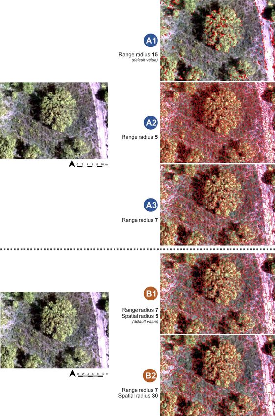
Figure4.4. Visual
Figure Visual comparison
comparison fromfrom some
some ofof the
the numerous
numerous tests
tests carried
carried out
outfor
forthe
theestimation
estimationofof
segmentation accuracy. On the left, a portion of the R-G-NIR image is shown; on the right,the
segmentation accuracy. On the left, a portion of the R-G-NIR image is shown; on the right, thesame
same
area is shown with the superimposed vector file containing the segmentation polygons
area is shown with the superimposed vector file containing the segmentation polygons (segments). (segments).
The
The top
top images,
images, from
from A1A1to to
A3,A3, show
show thethe segmentation
segmentation results
results obtained
obtained without
without thethe smoothing
smoothing step
step and
a and
rangea radius
range of
radius of default
15 (the 15 (thevalue),
default5,value), 5, and
and 7. The 7. The
lower lower
images, B1 images, B1 and
and B2, show theB2, show the
segmentation
segmentation
results with theresults with step
smoothing the smoothing
and a spatialstepradius
and a of
spatial
5 (theradius
defaultof value)
5 (the default
and 30.value) and 30.Remote Sens. 2019, 11, 1238 12 of 22
Remote Sens. 2019, 11, x FOR PEER REVIEW 12 of 22
TheTheevaluation
evaluationofofdifferent
differentcombinations
combinations of these parameters,
of these parameters,and andtherefore
thereforeofofthethe obtained
obtained
segmentations, was performed by means of visual interpretation by superimposing
segmentations, was performed by means of visual interpretation by superimposing them over them overthethe
orthomosaic.
orthomosaic.We Weobtained
obtainedthe
themost
most satisfactory resultsafter
satisfactory results aftersetting
settingthe
therange
rangeradius
radius value
value to to 7 and
7 and
thethe
size of tiles to 500 × 500 pixels. These values proved to be the most reliable for both
size of tiles to 500 × 500 pixels. These values proved to be the most reliable for both spring and spring and
summer imagery. The region merge step followed the segmentation stage, from
summer imagery. The region merge step followed the segmentation stage, from which 26,815 and which 26,815 and
49,575
49,575segments
segmentswerewereobtained
obtainedfor
forthe
the spring
spring and summer
summerflights,
flights,respectively.
respectively.Figure
Figure 4 shows
4 shows a set
a set
of of
examples
examplesofofthe thesegmentation
segmentationprocedure
procedure with the the superimposition
superimpositionofofthe thevector
vectorfile
file containing
containing
segments
segments onon the
the RGBimage
RGB imagefrom
fromaasmall
smallportion
portion of the study
study area.
area.
4.3.4.3.
Classification
Classificationand
andAccuracy
AccuracyAssessment
Assessment
In In
thethe training
training phase,
phase, 586586 polygons
polygons forfor
thethe spring
spring image
image andand
10671067 polygons
polygons for summer
for the the summer
image
image (corresponding to 2.18% and 2.15% of the total number, respectively) were
(corresponding to 2.18% and 2.15% of the total number, respectively) were selected. Details on selected. Details onthe
the surface
surface distribution
distribution and spectral
and spectral characteristics
characteristics of the
of the training
training and
and validationpolygons
validation polygons according
according to
thetofive
theland-use
five land-use classes
classes are provided
are provided in Appendix
in Appendix A (Tables
A (Tables A3 and
A3 and A4).A4).
TheThe
twotwo resulting
resulting landland
cover
cover maps are shown in
maps are shown in Figures 5 and 6. Figures 5 and 6.
Figure
Figure 5. 5. Mapsofofthe
Maps theland
landcover
coverclassification
classification for
for the
thespring
springflight
flightobtained
obtainedfrom
fromrandom
random forest (RF)
forest (RF)
(A1)
(A1) and
and supportvector
support vectormachine
machine(SVM)
(SVM) (A2)
(A2) algorithms.
algorithms. Bar
Barcharts
chartsshow
showthe
thesurface distribution
surface distribution
according
according toto the
the fivedefined
five definedland
landcover
coverclasses.
classes.39% for SVM (38.95% spring, 38.58% summer). The shrubs class represents about 10% according to
RF in both spring and summer imagery, while for the SVM algorithm, shrubs form about 12% of the
classified area. The grass class accounts for about 32.5% of the area (32.83% RF, 32.24% SVM) from
the spring flight, while for the summer flight, this value is about 29% (28.95% RF, 29.22% SVM).
Shadows cover 15.03% (RF) and 14.91% (SVM) in the spring image, while in the summer image,
Remote Sens. 2019, 11, 1238 13 of 22
shadows amount to just over 19% (19.23% RF, 19.47% SVM). The class representing bare soil does not
exceed 1.62%.
Figure 6.
Figure Maps of
6. Maps of the
the land
land cover
cover classification
classification for
for the
the summer
summer flight
flight obtained
obtained from
from random
random forest
forest
(RF) (B1) and support vector machine (SVM) (B2) algorithms. Bar charts show the surface distribution
(RF) (B1) and support vector machine (SVM) (B2) algorithms. Bar charts show the surface distribution
according to
according to the
the five
five defined
defined land
land cover
cover classes.
classes.
The incidence of the cork oak class is almost the same for both classifiers and in both flights, with
Table 3 reports the confusion matrices for the accuracy assessment, while Table 4 reports the
values ranging between just over 40% for the RF classifier (40.10% spring, 40.31% summer) and nearly
kappa values and the overall accuracy for both RF and SVM classification algorithms and for both
39% for SVM (38.95% spring, 38.58% summer). The shrubs class represents about 10% according to
spring and summer flights. On the basis of 479 and 393 validation polygons for spring and summer
RF in both spring and summer imagery, while for the SVM algorithm, shrubs form about 12% of the
flights, respectively, the user’s accuracy for the cork oak class is 97.37% (spring) and 98.73% (summer)
classified area. The grass class accounts for about 32.5% of the area (32.83% RF, 32.24% SVM) from the
for RF, while for SVM it is 98% (spring) and 96.18% (summer). The values of the producer's accuracy
spring flight, while for the summer flight, this value is about 29% (28.95% RF, 29.22% SVM). Shadows
are 98.67% (spring) and 95.68% (summer) for RF, and 98% (spring) and 97.42% (summer) for SVM.
cover 15.03% (RF) and 14.91% (SVM) in the spring image, while in the summer image, shadows amount
For the shrubs class, the user's accuracy of the RF classifier is between 80% (summer) and about 98%
to just over 19% (19.23% RF, 19.47% SVM). The class representing bare soil does not exceed 1.62%.
Table 3 reports the confusion matrices for the accuracy assessment, while Table 4 reports the
kappa values and the overall accuracy for both RF and SVM classification algorithms and for both
spring and summer flights. On the basis of 479 and 393 validation polygons for spring and summer
flights, respectively, the user’s accuracy for the cork oak class is 97.37% (spring) and 98.73% (summer)
for RF, while for SVM it is 98% (spring) and 96.18% (summer). The values of the producer’s accuracy
are 98.67% (spring) and 95.68% (summer) for RF, and 98% (spring) and 97.42% (summer) for SVM.Remote Sens. 2019, 11, 1238 14 of 22
For the shrubs class, the user’s accuracy of the RF classifier is between 80% (summer) and about 98%
(spring), and for SVM it is about 90% in the spring flight, while it dropped to 66% in the summer flight.
Table 3. Confusion matrices for both classification algorithms, random forest (RF) and support vector
machines (SVM), and for both flights (spring and summer). Land cover classes are denoted as follows:
1 = cork oak; 2 = shrubs; 3 = grass; 4 = soil; 5 = shadows.
Ground Truth
RF Spring Total User’s accuracy
1 2 3 4 5
1 148 1 3 0 0 152 97.37%
2 1 104 1 0 0 106 98.11%
Classified 3 0 0 43 2 0 45 95.56%
4 0 0 0 8 0 8 100%
5 1 0 1 0 96 98 97.96%
Total 150 105 48 10 96 479
Producer’s accuracy 98.67% 99.05% 89.58% 80% 100%
Ground Truth
SVM Spring Total User’s accuracy
1 2 3 4 5
1 147 1 2 0 0 150 98%
2 2 96 7 1 0 106 90.57%
Classified 3 1 8 38 1 0 48 79.17%
4 0 0 0 8 0 8 100%
5 0 0 1 0 96 97 98.97%
Total 150 105 48 10 96 479
Producer’s accuracy 98% 91.43% 79.17% 80% 100%
Ground Truth
RF Summer Total User’s accuracy
1 2 3 4 5
1 155 0 2 0 0 157 98.73%
2 5 40 2 0 3 50 80.00%
Classified 3 0 0 97 0 1 98 98.98%
4 0 0 2 5 0 7 71.43%
5 2 0 3 0 75 80 93.75%
Total 162 40 106 5 79 392
Producer’s accuracy 95.68% 100% 91.51% 100% 94.94%
Ground Truth
SVM Summer Total User’s accuracy
1 2 3 4 5
1 151 1 3 0 2 157 96.18%
2 1 33 10 0 6 50 66%
Classified 3 0 1 94 0 3 98 95.92%
4 0 0 2 5 0 7 71.43%
5 3 10 1 0 66 80 82.50%
Total 155 45 110 5 77 392
Producer’s accuracy 97.42% 73.33% 85.45% 100% 85.71%
Table 4. Kappa index and overall accuracy for both classification algorithms, random forest (RF) and
support vector machine (SVM), and for both flights (spring and summer).
Imagery Kappa Value Overall Accuracy
RF Spring 0.973 97.6%
SVM Spring 0.935 94.1%
RF Summer 0.928 94.9%
SVM Summer 0.847 89.0%
A similar difference is registered for the producer’s accuracy, whose values are close to 100%
for RF, while for SVM, they are 91.43% and 73.33% in spring and summer, respectively. The grass classRemote Sens. 2019, 11, 1238 15 of 22
is classified with a user’s accuracy of 95.56% (spring) and 98.98% (summer) for RF and 79.17% (spring)
and 95.92% (summer) for SVM.
The producer’s accuracy reaches 89.58% (spring) and 91.51% (summer) with RF, and 79.17%
(spring) and 85.45% (summer) for SVM. Table 4 indicates an overall accuracy of 97.6% for RF and
94.1% for SVM in the spring image, with kappa values ranging from 0.973 to 0.935 for RF and SVM,
respectively. The overall accuracy for the summer mosaic is 94.9% for RF and 89% for SVM, with kappa
values of around 0.928 for RF and 0.847 for SVM.
Both classifiers (RF and SVM) did not require particular computational resources. Both imagery
classification steps, including the training phase, took a few seconds (from 1 to 10 seconds; in this
computing time, we excluded the selection of trainers that we performed manually).
5. Discussion
5.1. Segmentation
Given that it was expected to worsen the results, the smoothing step of the standard segmentation
workflow provided in OTB was omitted because it reduces the contrast necessary to discriminate
between the cork oak and shrub classes. The optimization of the range radius and minsize values led
to a consistent separation between cork oak, shrubs, and grass classes.
To accomplish the segmentation step with the high structural and compositional heterogeneity of the
site, we adopted a low-scale factor of objects, and this was effective. Actually, in the LSMS-segmentation
algorithm, the scale factor can be only managed through the adopted values of the range radius and
minimum region size parameters. As reported by scholars [56–59], even today, the visual interpretation
of segmentation remains the recommended method to assess the quality of the obtained results.
Taking into account the high geometrical resolution of our imagery (i.e., GSD = 10 cm), a low scale
of segmentation was preferable; thus, relatively low values of the range radius and minimum region
size were used. Even though producing very small segments, in some cases, leads to over-segmentation
(i.e., a single semantic feature is split into several segments, which then need to be merged), a low scale
of objects effectively resulted in a high degree of accuracy. It allowed the identification of polygons
that represent every small radiometric difference in tree crowns, as well as small patches of grass and
shrubs (Figure 3). As highlighted in several studies [29,60–62], a certain degree of over-segmentation
is preferable to under-segmentation to improve the classification accuracy, as can be clearly inferred
from the results in Tables 3 and 4.
It is important to underline a very significant difference in the number of polygons in the
segmentation results of the two different mosaics, despite our application of region merging using
the same threshold size (250 pixels). As shown in the results section, the summer image presents
almost twice the number of polygons relative to the spring image. This might be explained by a higher
chromatic difference caused by a high contrast of vegetation suffering from drought (especially Cistus
and the herbaceous layer) and by an increased presence of shadows (an increase of more than 4% of
the study area compared with the spring image). Actually, the summer flight was performed earlier
in the day (11:00) than the spring one (13:00), so the flights were subjected to different sun elevation
angles (Table A1). Nevertheless, Figure 3 shows that the obtained segmentation correctly outlines
the boundaries of the tree crowns, as well as the shrub crowns and the surrounding grass spots,
discriminating one from the other. The segmentation results also clearly differentiate between the
bare soil and the vegetation, even in the presence of small patches. As reported in recent studies that
performed forest tree classification [18,59], the additional information provided by the DSM and NDVI
significantly improves the delimitation and discrimination of segments, which was true in our case
as well. This is more relevant in conditions in which the three vegetation layers are spatially close,
because discrimination based only on spectral information has proven very difficult to achieve in such
environments. An additional detail to mention is that the algorithm was able to accurately recognize
the shadows, an important “disturbing factor” for image processing, since they are usually hardlyRemote Sens. 2019, 11, 1238 16 of 22
distinguished from other objects. This is the reason why shadows were specifically considered as
a separate class category.
5.2. Classification and Accuracy Assessment
The GEOBIA paradigm coupled with the use of machine learning classification algorithms is
currently considered an excellent “first-choice approach” for the classification of forest tree species
and the general derivation of forest information [28,31,41,55,63]. As reported by Trisasongko et al. [55]
and Immtzer et al. [41] and confirmed in this study, the default values of the OTB parameters for
training and classification processes provide optimal results, and they were maintained in the final test.
Moreover, both classifiers were very fast, requiring just around 10 seconds for their execution.
Generally, the quality of the classification can be considered good according to the quality errors,
which are intrinsic to the image. This is confirmed by the kappa coefficient, whose values ranged
from 0.928 to 0.973 for RF and from 0.847 to 0.935 for SVM. For both spring and summer imagery,
the comparison between the SVM and RF algorithms does not reveal large differences in the classification
maps, and any differences detected are in very small polygons. However, a comparison of the kappa
results with the overall accuracy reveals that the RF algorithm turns out to be more accurate than SVM
for both flights, and this is also reflected by the confusion matrix. The most repeated error, particularly in
the images classified with SVM, is confusion between the shrubby class and the shadows class, limited to
the edges of the shadows. On the contrary, shrubs are clearly distinguished from tree crowns in the
whole scene.
The classes, if taken independently, can be analyzed through the user’s and the producer’s
accuracy, which indicate commission and omission errors, respectively. For both flights and both
algorithms, the cork oak class obtains better classification accuracy, with values that are always higher
than 95%. On the other hand, the lowest accuracy is obtained for the shrubs class with the SVM
algorithm and the summer flight.
It can be noted from observing the confusion matrix that shrubs are more often confused with
shadows or herbaceous vegetation than they are with trees. A preliminary visual analysis is sufficient
to notice a common error in all of the maps: some polygons representing the edges of the shadows
(at which there is a chromatic transition from the shadow to the adjacent cover) are confused with
shrubs, but the confusion of shrubs with grass instead can be justified. It is hard to formulate a reliable
assessment of the results for the bare soil class because of the low number of samples, even if the result
is representative of the real distribution and width of the class in the whole region (Remote Sens. 2019, 11, 1238 17 of 22
for the same season leads to almost the same results, with small differences. Differences between the
seasons with the same classification algorithm can be also considered small, and the classifier does not
appear to be affected by the cyclical and biological behavior of the species. In fact, with the use of the
NDVI information layer, the algorithms similarly distinguished herbaceous vegetation from shrubs,
even if they were clearly affected by drought. The larger problem to be faced is related to the large area
of shadows in the summer mosaic.
6. Conclusions
Technological development for accurately monitoring vegetation cover plays an important role in
studying ecosystem functions, especially in long-term studies. In the present work, we investigated
the reliability of coupling the use of multispectral VHR UAV imagery with GEOBIA classification
implemented in OTB free and open-source software. Supervised classification was implemented by
testing two object-based classification algorithms, random forest (RF) and support vector machine (SVM).
The overall accuracy of the classification was optimal, with overall accuracy values that never fell
below 89% and kappa coefficient values that were at least 0.847. Both classifiers obtained good levels
of accuracy, although the RF algorithm provided better results than SVM for both images. This process
does not seem to have been examined in previous studies; as far as we are aware, this study is the first
that uses multispectral R-G-NIR images with DSM and NDVI for the classification of forest vegetation
from UAV images using open-source software (OTB).
An open question worth investigating relates to the application of our findings to other forest
ecosystems. The OTB suite is free and open-source software that is regularly updated and has proven
to provide free processing tools with a steep learning curve coupled with robust results in forest
ecosystems that have a complex vertical and horizontal structure. Moreover, as our findings show,
OTB can effectively process UAV imagery when implemented on low-power hardware. Therefore,
the proposed workflow may be highly valuable in an operational context.
However, some open questions and future research directions remain worthy of investigation.
On the one hand, further investigation into the use of smoothing to try to optimize potential usefulness
should be carried out in different operational conditions. On the other hand, for the issue with tree
shadows, our experience in this study reveals that flight schedules can significantly affect the quality of
the obtained imagery, especially in open forest ecosystems such as cork oak woodlands. The summer
imagery is affected by about 30% more shadowed area than the spring one.
Our findings confirm the reliability of UAV remote sensing applied to forest monitoring and
management. Moreover, although a massive amount of UAV hyperspectral and LiDAR data can be
obtained with ultra-high spatial and radiometric resolutions, these sensors are still heavy, too expensive,
and in most cases require two flights to obtain radiometric and topographic information. Our sensor,
which is based on standard R-G-NIR imagery, has the significant advantage of being a very affordable
solution in both scientific and operational contexts. Additionally, mounting this sensor on a fixed-wing
UAV enables the surveying of surfaces spread over hundreds of hectares in a short time and has thus
proven to be a very cost-effective and reliable solution for forest monitoring.
Author Contributions: Conceptualization, J.M.N.S., S.C., and G.M.; methodology, G.D.L., J.M.N.S., and G.M.;
formal analysis, G.D.L., J.M.N.S., and G.M.; investigation, G.D.L.; data curation, G.D.L., J.M.N.S., J.A. and G.M.;
writing—original draft preparation, G.D.L., J.M.N.S., S.C. and G.M.; writing—review and editing, all the authors.
Funding: G.D.L. was funded by the European Union Erasmus+ program (Erasmus+ traineeship 2017–2018
Mobility Scholarship). We would like to thank the support from the MEDSPEC project (Monitoring Gross Primary
Productivity in Mediterranean oak woodlands through remote sensing and biophysical modelling), funded
by Fundação para a Ciência e Tecnologia (FCT), Ministério da Ciência, Tecnologia e Ensino Superior, Portugal
(PTDC/AAG-MAA/3699/2014). CEF is a research unit funded by FCT (UID/AGR/00239/2013).
Acknowledgments: Authors acknowledge the Herdade da Machoqueira do Grou for permission to undertake
this research. The authors would like to express their great appreciation to the four anonymous reviewers for their
very helpful comments provided during the revision of the paper.Remote Sens. 2019, 11, x FOR PEER REVIEW 18 of 22
Conflicts
Remote of Interest:
Sens. 2019, 11, 1238 The authors declare no conflict of interest. The funders had no role in the design of the22
18 of
study; in the collection, analyses, or interpretation of data; in the writing of the manuscript, or in the decision to
publish the results.
Conflicts of Interest: The authors declare no conflict of interest. The funders had no role in the design of the
Appendix
study; A
in the collection, analyses, or interpretation of data; in the writing of the manuscript, or in the decision to
publish the results.
Table A1. Meteorological conditions characterizing the two flights (spring and summer).
Appendix A
Flight Sun Sun
UTC Reference Takeoff Landing Wind
Date Duration Elevation Azimuth
Table A1.
ZoneMeteorological
Time conditions
LT characterizing
LT the two flights (spring and summer).
Conditions
(minutes) (deg) (deg)
Flight Sun Sun
05-04-2017 UTC+1
UTC 13:00
Reference 12:37
Takeoff 13:18
Landing 41 Strong
Wind 56.14 163.81
Date Duration Elevation Azimuth
Zone Time LT LT Conditions
13-07-2017 UTC+1 11:00 10:49 11:17 28
(minutes) Light 51.97
(deg) 105.33
(deg)
05-04-2017 UTC+1 13:00 12:37 13:18 41 Strong 56.14 163.81
13-07-2017 UTC+1 11:00 10:49 11:17 28 Light 51.97 105.33
Table A2. Main technical specification of the workstation used for data processing.
Model Main
Table A2. Dell technical
Precision specification
Workstation T7500 of the workstation used for data processing.
Processor Intel Xeon CPU E5503 @ 2.00 GHz, 1995 MHz, 2 Kernels, 2 Logical Processors
Model
RAM installed
Dell Precision Workstation T7500
6.00 GB
Processor
System Type x64-based Xeon
Intel PC CPU E5503 @ 2.00 GHz, 1995 MHz, 2 Kernels, 2 Logical Processors
RAM installed 6.00 GB
System Type x64-based PC
Figure A1.Spectral
A1.
Figure Spectralsignature
signatureofofcork
corkoaks
oaksin
in spring
spring and
and summer UAV imagery
summer UAV imagery (green,
(green,red,
red,and
andNIR
NIR
bands). The transparent area shows minimum and maximum values
bands). The transparent area shows minimum and maximum values range. range.
Table A3. Surface distribution of training and validation polygons according to the five defined land
cover classes. Land cover classes are denoted as follows: 1 = cork oak; 2 = shrubs; 3 = grass; 4 = soil;
5 = shadows.
Table A3. Surface distribution of training and validation polygons according to the five defined land
cover classes. Land cover classes are denoted as follows: 1 = cork oak;Validation
Trainers 2 = shrubs; 3 = grass; 4 = soil; 5
= shadows. Spring Summer Spring Summer
Class Area [ha] Area [ha]
Trainers AreaValidation
[ha] Area [ha]
1 0.1119 0.0963 0.1257 0.05
Spring Summer Spring Summer
2 0.0586 0.0891 0.0599 0.01
Class
3 Area [ha]
0.6017 Area [ha]
0.2095 Area [ha]
0.8970 Area [ha]
0.490
41 0.0702
0.1119 0.0258
0.0963 0.0162
0.1257 0.022
0.05
52 0.0613
0.0586 0.0759
0.0891 0.0473
0.0599 0.032
0.01
Number of polygons 586 1067 479 393
3 0.6017 0.2095 0.8970 0.490
4 0.0702 0.0258 0.0162 0.022
5 0.0613 0.0759 0.0473 0.032
Number of polygons 586 1067 479 393You can also read