Living Cost Gap in the European Union Member States - MDPI
←
→
Page content transcription
If your browser does not render page correctly, please read the page content below
sustainability

Article
Living Cost Gap in the European Union
Member States
Andrius Kučas * , Boyan Kavalov and Carlo Lavalle
 European Commission, Joint Research Centre (JRC), 21027 Ispra, Italy; boyan.kavalov@ec.europa.eu (B.K.);
 carlo.lavalle@ec.europa.eu (C.L.)
 * Correspondence: andrius.kucas@ec.europa.eu; Tel.: +39-033-278-9445

 Received: 16 September 2020; Accepted: 24 October 2020; Published: 28 October 2020

 Abstract: The living cost gap refers to the differential amongst income, expenditures, and poverty
 lines. It is important since it addresses a number of aspects that point towards historic and continued
 living standards. The purpose of this study is to identify, measure, and compare the living cost
 gap in the Europe Union member states. Twenty-nine indicators/criteria from Eurostat and World
 Bank, covering the period 2008–2017, are employed. In order to rank and compare living cost gap
 by countries, objective functions for each criterion are defined and applied. The importance of each
 criterion is assessed independently. The composite living cost gap indicator for each MS is calculated
 using multiple criteria decision support methods. The relationship between the compound annual
 growth rates of this indicator and each single criterion is estimated and evaluated. The findings of the
 study suggest that living cost gap is higher where unemployment rates and households’ expenditure
 on basic needs (housing, food etc.), are larger, while living cost gap is lower where households’ income
 and expenditure on optional needs are higher. The living cost gap in the majority of countries tends
 to narrow/decrease, along with the increase in the household income and expenditures. Our research
 highlights the need to mitigate unemployment and households’ low net income in order to alleviate
 living cost gap. The analysis and assessment of living cost gap might help identifying the most
 vulnerable social profiles and groups, and hence might contribute to the adequate formulation
 and implementation of targeted policy responses and interventions at European Union, national,
 and regional level.

 Keywords: household; income; expenditures; multiple-criteria decision making; compound annual
 growth rate

1. Introduction
     Territorial inequalities have long been studied and dealt with in the literature and in policy [1–8],
but still many research questions remained unanswered and many issues unsolved [9]. Therefore,
there is historical and continuous interest to analyse territorial disparities through new lenses and
produce knowledge useful to understand the cost of living combining the characteristics of places and
social connections [10]. By definition, the cost of living is the amount of money needed to sustain a
certain standard of living by affording basic expenses. An increasing divergence in living standards
and costs is being recently observed across Europe, partially because much of Europe’s economic
growth has been uneven, mostly occurring in larger regions [8,11].
     The notion ”Living Cost Gap” (LCG) refers to the differential amongst income [12,13],
expenditure [14,15], employment [16–18], and poverty [19,20], usually aggravated by economic
crises and recessions [20–23].

Sustainability 2020, 12, 8955; doi:10.3390/su12218955                      www.mdpi.com/journal/sustainability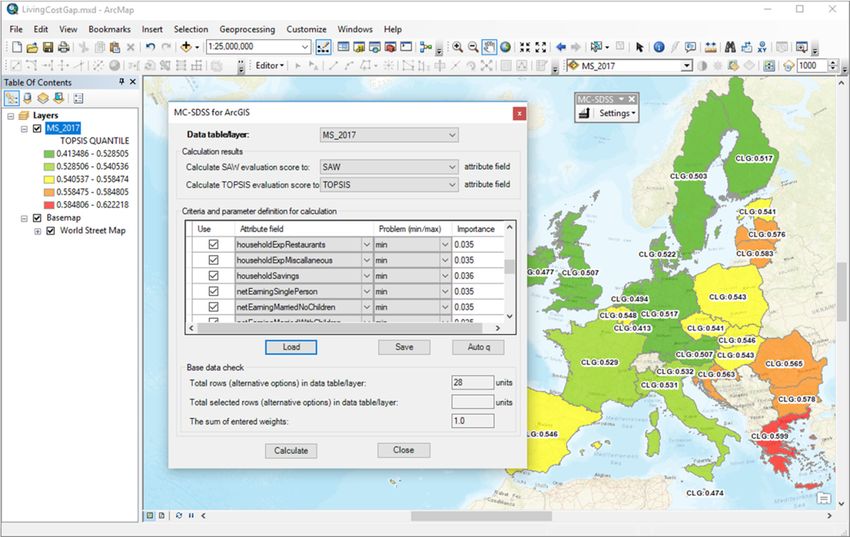
Sustainability 2020, 12, 8955                                                                         2 of 26

      The LCG challenge is important since it addresses a number of aspects that point towards a
historic and continued living standards and expected stress-related behaviour when the living cost
burden occurs [20,24–27].
      The most attractive places to live are generally defined by the optimum ratio between income
and expenses [28,29]. Other factors such as housing conditions and life satisfaction [25], personal
safety and security [26], availability of good transport infrastructure [30], education [28], attractive
labour market [31], and reduced risk of poverty [20,32] might be considered as additional benefits for
the households.
      Due to a generally favourable combination of those factors, people tend to live in urbanised areas
(cities, towns, or suburbs). Consequently, the non-urbanised (rural) areas are becoming less populated.
Amongst others, this is due to the consolidation of innovation-driven and efficient production toolsets
in the primary sector (agriculture, forestry and fisheries) that largely dominates the economy of rural
areas. This phenomena reduces the labour demand, resulting in declining employment and retarded
growth of rural income [33]. It is not very likely that growth in secondary and tertiary sectors of
economy in rural areas can solve poverty problems in the foreseeable future, especially in many
backward regions [34]. On the other hand, the negative impacts in large cities, such as labour crowding
and elevated cost of living, may boost the appeal of smaller urban centres and rural regions [11].
      It is therefore important to monitor the evolution of those factors taken altogether, i.e., territorial
volatility, while urban areas expand and population increases. In such a way, one prevents attractive
areas to transform into less attractive or unattractive ones due to fewer and/or poorer job offers, higher
risk of poverty, and less affordable living cost. The lack of job opportunities and thus sufficient income
to guarantee a minimum standard of living or even–minimum level for surviving, leads to poverty,
deprivation, and ultimately boosts LCG.
      The rising awareness of the negative effects from urban poverty, followed by LCG, has resulted in
a rapidly increasing number of requests for new policy incentives aimed at reducing the risk of poverty
and vulnerability, more affordable living cost costs, more and better opportunities for employment,
and income earning [19,35]. In a broader context, there is growing demand for comprehensive scientific
knowledge and tools to enhance environmental, economic, and social values of separate processes
by managing them in accordance with the principles of integrated sustainability [36]. However,
decision-makers often deal with problems that involve multiple conflicting criteria [37–40]. Closing or
at least narrowing the LCG is a challenging and complex process that requires evaluation of many
diverse criteria, alongside with geospatial analysis. The identification of the living cost component of
LCG is the first step in tackling the LCG challenge. Comprehensive studies to detect LCG in the EU
Member States (MS) seem to be largely missing.
      The multi-criteria spatial decision support techniques have been chosen for the purpose of this
study, since they allow multiple criteria-based ranking of MS by using tightly integrated [37] geographic
information systems (GIS) and multiple criteria decision-making (MCDM) approaches, along with
general decision support input concerning analytical approaches and interpretations.
      The overall purpose of this study is therefore to:

1.     Develop flexible LCG identification framework, which could help decisions-makers in preparation
       of LCG mitigation measures;
2.     Identify LCG change trends across MS;
3.     Provide solution to identify which criterion (and under which circumstances) become more
       important for identification of LCG;
4.     Estimate and evaluate relationship between compound annual growth rates (CAGR) of LCG and
       CAGR of each criterion, across MS.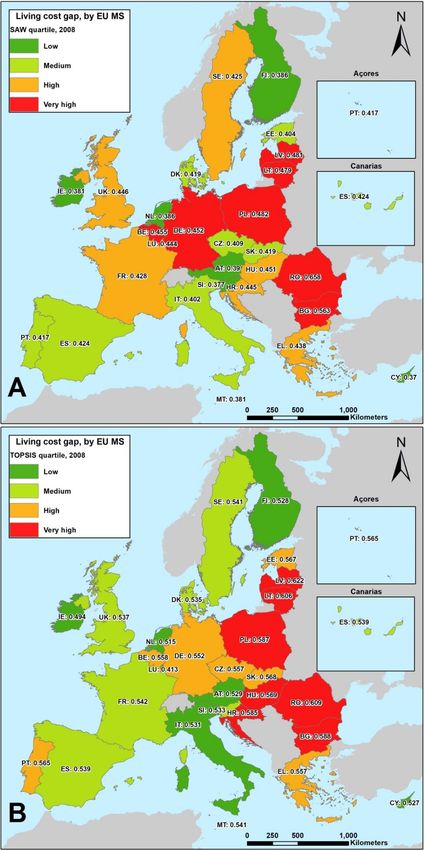
Sustainability 2020, 12, 8955                                                                      3 of 26

2. Materials and Methods

2.1. Study Area and Source Data Preparation
      Open and publicly available data from Eurostat and World Bank for the period 2008–2017
(Table A1) were used for the identification of LCG in the 28 MS, assessed in this study and to create the
composite LCG indicator.
      The methodology comprised of 27 Eurostat [41–53] and 2 World Bank [54] indicators (called
“criteria” in our study) at national level that were aggregated and processed in order to assess the LCG
in the MS and consequently, to allow for comparison of LCG across MS.
      For further analysis, all criteria were grouped based on criteria relationship with the households.
Four criteria and household relationship types were defined and applied for grouping:

•     Hypothetical distance from household: adjacent, neighbouring, and distant;
•     Economic decision scale relationship with household: micro, mezzo, macro;
•     Location effect on household: local, national, international;
•     Impact of decision makers on household: individual, external.

     Criterion and household relationship type can be described by spatial-temporal means. The criteria
that might be impacted by decisions made at household level (e.g., net income, savings) are more
adjacent than the criteria that cannot be impacted by decisions made at household level with immediate
effect (e.g., labour market, gross domestic product (GDP), trade flows, etc.) on living standards.
     Based on the relationship type, we grouped these determinants (criteria) into three categories
(Table A2), as follows:

•     Adjacent–micro–local–individual (e.g., household net earnings, savings);
•     Neighbouring–mezzo–national–external (e.g., GDP, labour market, housing availability);
•     Distant–macro–international–external (e.g., migration, remittance flows, trade flows);

     Adjacent–micro–local–individual group was subsequently broken down into further three
sub-categories (Table A2), as follows: income, basic, and optional expenditures;
     Criteria grouping enabled separate evaluation and objective function definition (addressing the
highest LCG) for each criterion (Table A2).
     The overall input data preparation was orchestrated in order to find the highest LCG across MS,
detect changes in LCG between 2008 and in 2017 respectively (Table A2), and find the indicators that
impact LCG the most.

2.2. The LCG Assessment Framework
     The objective criterion importance [55] has been calculated based on selected
minimization/maximization functions. The function to maximize/minimize has been called “objective
function.” Criterion importance values (Table A3) have been then used as an input for the ranking
of MS using simple additive weighting (SAW) and technique for order preference by similarity to
ideal solution (TOPSIS) techniques [38]. The two methods have been applied for result validation
reasons and also because they employed the same inputs, but via two different ranking approaches.
The ranking outcomes have been considered reliable if both methods had generated similar results.
The final SAW and TOPSIS values ranged from 0 (worst) to 1 (best) and altogether built the so-called
composite LCG indicator. A higher rank value means higher LCG. The SAW and TOPSIS values for
each MS have been separately calculated for 2008 and 2017 (Tables A4 and A5) and later compared
with each other.
     The so-identified composite LCG and LCG changes were visualized on a map by using quartile
mapping technique to facilitate LCG comparisons amongst countries. In order to better understand
which criterion had the strongest impact on LCG change, we calculated compound annual growth rates
(CAGR) [56] of SAW (Table A4), TOPSIS (Table A5), and for all criteria (Table A6). Finally, we checked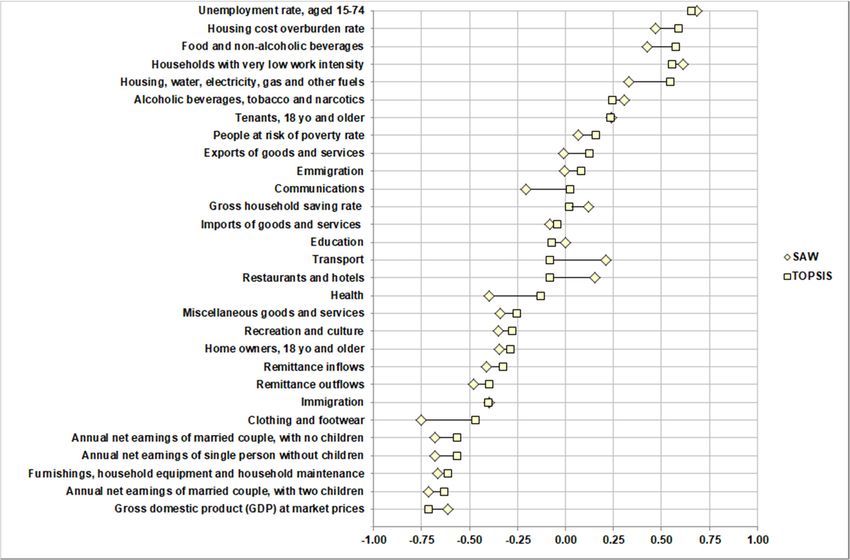
Sustainability 2020, 12, 8955 4 of 26
the relationship (Pearson correlation) between CAGR of each criterion and CAGRs of SAW (Table A4)
and TOPSIS (Table A5) across MS (Table A6).
A Unified Modelling Language [57] based sequence diagram illustrates workflow and describes
all data and information flows within the framework (Figure 1).
Sustainability 2020, 12, x FOR PEER REVIEW 4 of 29
Figure1.1.Decision
Figure Decisionflowchart
flowchartfor
formultiple
multiplecriteria
criteriaanalysis
analysisofofLCG.
LCG.
Theadvanced
The advanced level
level license ofof ArcGIS
ArcGISDesktop
Desktopversion
version10.6
10.6software
softwaredeveloped
developed by by
ESRI Inc.,
ESRI
Redlands,
Inc., CA, CA,
Redlands, USA,USA,
has been applied
has been for data
applied for analyses and mapping.
data analyses and mapping.To calculate the objective
To calculate the
importance
objective of criteria
importance of and country’s
criteria LCG ranks,
and country’s LCGa ranks,
customa SDSS
custom[58], MC-SDSS
SDSS for ArcGIS
[58], MC-SDSS for software
ArcGIS
extension
software [55], has[55],
extension beenhas
used (Figure
been used A1). ThisA1).
(Figure extension implements
This extension full decision-making
implements workflow
full decision-making
(Figure A2)
workflow including
(Figure calculation
A2) including of criteria
calculation importance,
of criteria SAW,SAW,
importance, and and
TOPSIS values
TOPSIS within
values GIS
within
environment.
GIS environment.
2.3.
2.3.Definition
DefinitionofofLCG
LCGUsing
UsingObjective
ObjectiveFunctions
Functions
AAUnified
UnifiedModelling
ModellingLanguage
Language[57]
[57]based
basedsequence
sequencediagram
diagramillustrates
illustratesworkflow
workflowand anddescribes
describes
allalldata
dataand
andinformation
informationflows
flowswithin
withinthe
theframework
framework(Figure
(Figure1).1).
Household
Householdmanagement
managementdecisions
decisionsarearetypically
typicallyguided
guidedby bymultiple
multipleobjectives
objectivesmeasured
measuredinina a
range
rangeofoffinancial
financialand
andnon-financial
non-financialcriteria.
criteria.InInorder
ordertotoperform
performranking
rankingofofMS,
MS,thetheimportance
importanceofof
every
everycriteria has
criteria been
has calculated
been (Table
calculated A3)A3)
(Table based on the
based defined
on the objective
defined function
objective that addresses
function the
that addresses
LCG issue (Table A2).
the LCG issue (Table A2).
We assume that LCG is the highest where the following criteria (Table A1) and its objective
functions (minimization/maximisation) have been presented simultaneously across the MS (criteria
grouping according Table A2):
i. Households with lowest (minimisation) net income and lowest savings;
ii. Households with highest (maximisation) expenditures on basic needs (housing, food, and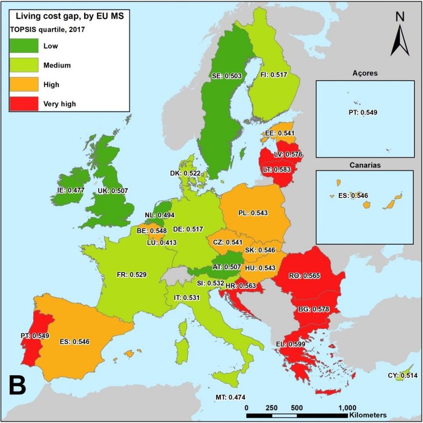
Sustainability 2020, 12, 8955                                                                              5 of 26

    We assume that LCG is the highest where the following criteria (Table A1) and its objective
functions (minimization/maximisation) have been presented simultaneously across the MS (criteria
grouping according Table A2):

i.       Households with lowest (minimisation) net income and lowest savings;
ii.      Households with highest (maximisation) expenditures on basic needs (housing, food,
         and transport) to maintain a minimum level of survival only;
iii.     Households with lowest (minimisation) expenditures on optional needs (education, health,
         clothing, other miscellaneous goods, etc.);
iv.      Households that are exposed to few employment opportunities and low GDP. MS where
         unemployment, low work intensity, and income poverty rates are the highest (maximisation)
         and GDP is lowest (minimisation);
v.       Households that are exposed to housing gap issues. MS where the housing cost overburden
         rate and the prevalence of rented houses are the highest (maximisation) and home ownership
         is the lowest (minimisation);
vi.      Households exposed to socio–economic challenges that only partially depend upon MS.
         MS where immigration, import of goods (MS expenditure) and remittance inflow (households
         demand for external support) are the highest (maximisation) and where emigration, export
         of goods (MS income), and remittance outflow (support capacity for households outside the
         country) are the lowest (minimisation).

      The detailed description of each indicator and its objective function (focusing on the “highest
LCG”) is provided in Table A2. To test the objective functions and the linkages amongst the criteria,
a criteria importance calculation algorithm [55] has been applied.

2.4. Calculation of Objective Criteria Importance
      Before calculating the criteria importance, we normalised the source data (Table A1) by adjusting
values measured on different scales to a notionally common scale using objective functions. The higher
the importance value qi [55], the more important the criterion is. All resulting criteria importance
values (Table A3) then have to be tested. The sum of importance values for all criteria has to be equal
to 1. This is a mandatory condition for further ranking via SAW and TOSPIS methods.
      In order to assess agreement (regarding LCG) amongst all criteria we used Kendall’s [59] coefficient
of concordance (Kendall’s W or W). W ranges from 0 (no agreement) to 1 (complete agreement). If W = 1,
then all the criteria are unanimous. If W = 0, then there is no overall agreement among the criteria
regarding LCG and criteria values may be regarded as random. Intermediate values of W indicate
greater or lesser degree of unanimity among various criteria considered (Table A3).
      In our study, W = 0.001 (for all criteria in Table A3) shows that criteria are still valid, but, there is no
overall agreement among the criteria regarding LCG. All criteria selected are essentially random (might
be also conflicting) and can be used for LCG identification across MS using SAW and TOPSIS methods,
because these two different methods are dedicated to cope with conflicting criteria. The calculation
of objective criteria importance values (including data normalisation and W) for each period was
performed using original objective criteria importance calculation algorithm [55] implemented within
custom made MC-SDSS for ArcGIS extension [55].

2.5. Calculation of LCG Using SAW Method
      The SAW method [38,60] is a multiple-criteria decision-making technique consisting of assigning
to each alternative a sum of values, each one associated to the corresponding evaluation criterion,
and weighted according to the relative importance of the corresponding criterion. The final SAW value
is calculated by summing up all the weighted criteria for certain alternatives. The input data used
for SAW calculations: MS as alternatives, normalised Eurostat, and World bank data as criteria and
criteria importance values (Table A3).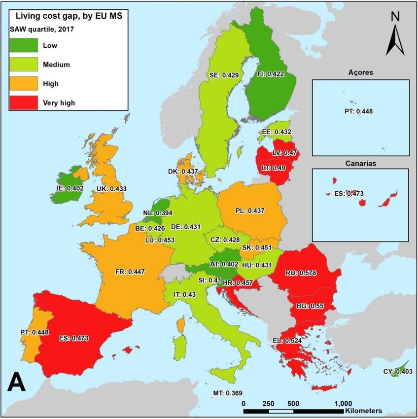
Sustainability 2020, 12, 8955                                                                        6 of 26

     The alternative (certain MS amongst all MS) that best fit the objective function (highest LCG) is
the one with the highest SAW value. MS with the lowest SAW values fit objective function (highest
LCG) the least, which means that such MS have lowest LCG (Table A4).

2.6. Calculation of LCG Using TOPSIS Method
     TOPSIS [38] defines a “similarity index” (relative proximity) by combining the geometric proximity
to the positive-ideal solution and the remoteness of the negative-ideal solution. The alternative that fits
the objective function (LCG) the best should have the shortest distance from the positive-ideal solution
and the longest distance from the negative-ideal solution. The input data used for calculations is the
same as in case of the SAW method that is described earlier.
     The alternative (certain MS amongst all MS) that best fit the objective function (highest LCG) is the
one with the highest TOPSIS value. MS with the lowest TOPSIS values fit objective function (highest
LCG) the least, which means that such MS have lowest LCG (Table A5).
     The calculation of SAW and TOPSIS values for each period and for each MS was performed
using SAW and TOPSIS calculation algorithms [38,60] implemented within custom made MC-SDSS for
ArcGIS extension [55].

3. Results

LCG and LCG Change Trends
     The analysis was focused on identifying the temporal LCG change within and across MS. In order
to address the LCG changes, we identified the LCG for the MS within the 2008–2017 period (Tables A4
and A5) by calculating SAW and TOPSIS values on annual basis. The maps show the SAW and TOPSIS
values (composite LCG indicator) for the baseline year 2008 (Figure 2A,B) and for the final year 2017
(Figure 3A,B).
     According the findings from (Figure 2A,B), the highest LCG in 2008, estimated along both methods,
was observed in two geographical parts of the EU—the Baltic Sea area (Latvia, Lithuania, and Poland)
and the Black Sea area (Romania and Bulgaria), while the lowest LCG was revealed in a more scattered
pattern, namely in Finland, Ireland, the Netherlands, Luxembourg, Austria, and Cyprus. It is worth
nothing that Belgium, Germany, Hungary, Croatia, and Greece appear also as countries with rather high
LCG. Combined with the results for the very high LCG, these observations mean that the whole Eastern
wing of the EU (except Cyprus), generally suffered of substantial LCG pressure in 2008. On the other
hand, Spain, Malta, Italy, Slovenia, and Denmark were peculiar with relatively low LCG. The picture
for the remaining EU countries assessed—Sweden, Estonia, Czechia, Slovakia, France, the United
Kingdom, and Portugal—was mixed. The following additional conclusions about LCG by 2008 could
be thereby revealed:

•     Estonia was more similar to Finland, rather than to the other two Baltic States;
•     The situation in the Benelux area was very diverse;
•     Czechia and Slovakia were rather similar;
•     The Southern layer of the EU, which in other contexts is often put together and demonstrates
      similarities, was very distinct.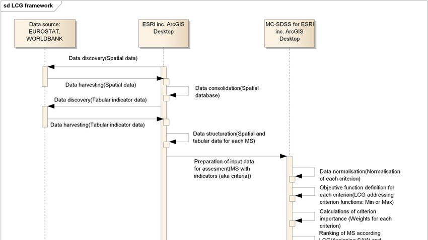
Sustainability 2020, 12, 8955                                                                              7 of 26
Sustainability 2020, 12, x FOR PEER REVIEW                                                                 7 of 29

      Figure 2.
      Figure 2. Quartile
                Quartile map
                         map of
                             of composite
                                composite LCG
                                            LCG indicator
                                                 indicator expressed
                                                           expressed in
                                                                      in SAW  (A) and
                                                                         SAW (A)  and TOPSIS
                                                                                       TOPSIS (B)
                                                                                              (B) values
                                                                                                  values for
                                                                                                         for
      2008 within
      2008 withinthe
                  theEU.
                      EU.Map
                          Maplabels
                                labelsdisplay:
                                       display:MS
                                                MS  name
                                                  name     abbreviation,
                                                        abbreviation,  SAWSAW  value
                                                                            value (A),(A),
                                                                                       andand TOPSIS
                                                                                           TOPSIS     value
                                                                                                  value (B).
      (B).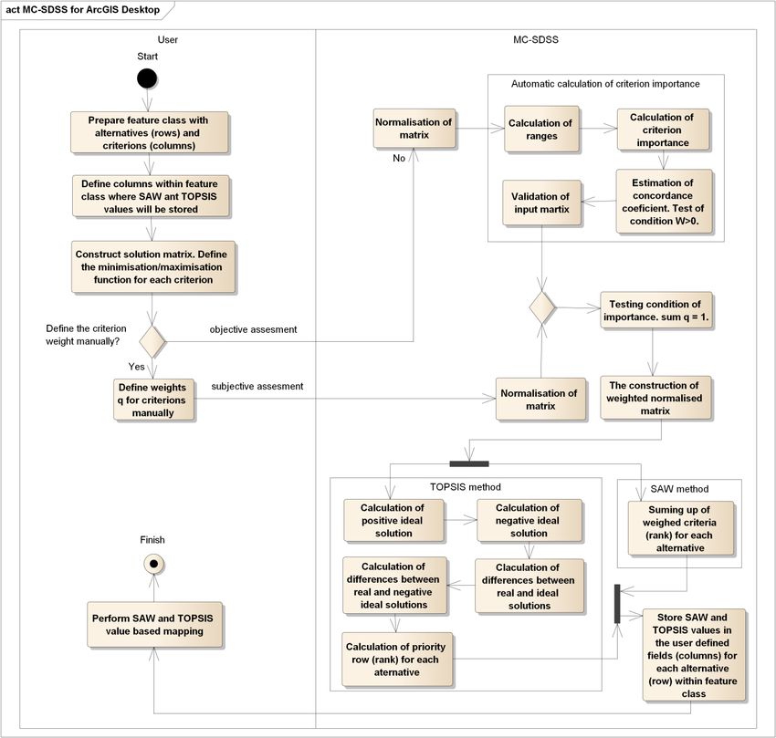
Sustainability 2020, 12, 8955                                                                              8 of 26
Sustainability 2020, 12, x FOR PEER REVIEW                                                                 9 of 29

      Figure
      Figure 3.
             3. Quartile
                Quartile map
                         map of
                             of composite
                                composite LCG
                                            LCG indicator
                                                 indicator expressed
                                                           expressed in
                                                                      in SAW
                                                                         SAW (A)
                                                                              (A) and
                                                                                  and TOPSIS
                                                                                       TOPSIS (B)
                                                                                              (B) values
                                                                                                  values for
                                                                                                         for
      2017 within the
      2017 within  theEU.
                       EU.Map
                          Maplabels
                                labelsdisplay:
                                       display:MS
                                                MSname
                                                    name  abbreviation,
                                                        abbreviation,  SAWSAW  value
                                                                            value (A),(A),
                                                                                       andand TOPSIS
                                                                                           TOPSIS     value
                                                                                                  value (B).
      (B).
Sustainability 2020, 12, 8955                                                                     9 of 26

     In 2017, the group of the countries with the highest LCG (Figure 3A,B) did not undergo major
modifications and again the two Baltic States (Latvia and Lithuania) and the two Black Sea EU members
(Romania and Bulgaria) landed there. Poland improved a little bit and went up to the group of high
LCG, but Greece and Croatia worsened and joined the club of the MS with the highest LCG. In such a
way, the very high LCG class got concentrated in the South-eastern wing of the EU, located on the
Balkan Peninsula. At the other end—the group of the lowest LCG—there were no major changes either.
Ireland, the Netherlands, Luxembourg, and Austria retained their membership. The downward LCG
change for Finland and Cyprus was negligible, while another small MS, Malta, substituted Cyprus
in this group. The LCG situation on the Iberian Peninsula (Portugal and Spain) worsened, while it
improved in Belgium, Germany, Poland, Hungary, Sweden, and to some extent in the United Kingdom.
The remaining MS assessed (France, Italy, Slovenia, Czechia, Slovakia, Denmark, and Estonia) did not
change much their relative LCG ranking.
     Besides the above relative ranking, the absolute LCG values, revealed along both SAW and TOPSIS
methods, suggests a more balanced situation across the EU. No extreme values (0 or 1) were ever
detected in any MS. The LCG values ranged between 0.38 and 0.66 both for 2008 and 2017, i.e., around
the mean of 0.5 (−0.13 and +0.16 respectively to the mean). This observation means that LCG existed
as a phenomenon even in the best performing (in terms of LCG) countries, but, on the other hand,
there were no MS really facing a dramatic LCG challenge. The similar ranges of SAW and TOPSIS
values also indicates that that so-revealed results are reliable, especially in the extreme cases, while
the sensitivity is obviously greater in the middle of the sample. Altogether, these findings imply with
quite some certainty that the LCG issue was relatively moderate in the EU both in 2008 and 2017.

4. Discussion

4.1. Possible Framework Advantages and Drawbacks
      Combining 29 indicators from different sources (Table A1) into a single multidimensional composite
indicator allows identifying the LCG, which otherwise would not be feasible by analysing those 29
indicators separately. The composite LCG indicator therefore reveals more comprehensively the critical
LCG across the EU than the separate statistical indicators alone.
      The basic variable inputs for both methods were the same, but different standardization/weighting
techniques might have led to slightly different results [61]. Ranking process could have resulted in
situations where certain criteria might have increased ambiguities in the decision-making process due
to insufficient information or contradicting judgments [61–63].
      The application of SAW and TOPSIS techniques should be more careful when a large number of
criteria are used. A high number of criteria in one assessment reduces and somehow equalises criterion
importance. In such a case, the solution matrix might become very sensitive and the results—not
plausible, since a small change in weighting and/or an error in observation data might result in very
sensitive ranking and consequently—alter the whole evaluation and ranking.
      In our study, LCG was calculated by employing the SAW and TOPSIS methods. Both methods
are fairly simple and appear as the most widely used multi-attribute decision techniques. The tightly
integrated GIS and MCDM components [40] allowed to run calculations simultaneously, share a
common database (Figure A2), and perform immediate analysis because the programme control
remained within the GIS when performing the MCDM analysis.
      We found that both SAW and TOPSIS methods were most accurate for the MS with the highest
and lowest LCG. In the remaining, more moderate cases, the LCG, calculated via SAW, was always
increasing (Table A4), while the LCG calculated along TOPSIS was decreasing (Table A5). It was
because the TOPSIS method is generally more accurate than the SAW method in calculating distances
from the extreme (best or worst) options [61].
      The results from our study can be interpreted at the national level only. The proposed
framework can be applied in the future also for LCG analyses at finer disaggregation (regional,
Sustainability 2020, 12, 8955 10 of 26
Sustainability 2020, 12, x FOR PEER REVIEW 11 of 29
European Commission’s LUISA Territorial Modelling Platform [64], backed up by the Urban Data
local, city/urban) level by ingesting additional socio-economic historic data and projections from the
Platform (UDP) [65] and/or other relevant data and information sources available at a more local
European Commission’s LUISA Territorial Modelling Platform [64], backed up by the Urban Data
level. The corresponding results and interpretation will obviously depend on the input data scope,
Platform (UDP) [65] and/or other relevant data and information sources available at a more local level.
coverage, quality, respective modifications and adjustments of the objective function, temporal
The corresponding results and interpretation will obviously depend on the input data scope, coverage,
accuracy and coherence, and finally–disaggregation levels.
quality, respective modifications and adjustments of the objective function, temporal accuracy and
coherence, and finally–disaggregation levels.
4.2. Criteria Importance Definition and Assessment
4.2. Criteria
In order Importance
to address Definition
the LCG, andwe Assessment
computed objective criteria importance based on input data
distribution
In orderand scattering
to address the [55].
LCG,Itwe is computed
recommended to exclude
objective criteriasimilar indicators
importance basedfrom the same
on input data
assessment. Strongly or perfectly positively correlated (Pearson) criteria
distribution and scattering [55]. It is recommended to exclude similar indicators from the same might also be redundant
and should Strongly
assessment. be excluded from positively
or perfectly multi-attribute analysis,
correlated because
(Pearson) they
criteria mayalso
might lead to misleading
be redundant and
interpretations, especially when the same objective function is applied for
should be excluded from multi-attribute analysis, because they may lead to misleading interpretations,perfectly correlated
criteria. Inwhen
especially our case, we used
the same (with
objective few exceptions)
function is applied indicators
for perfectly that had negligible
correlated criteria.orInmoderate
our case,
correlations.
we used (withThe strongest (indeed–perfect,
few exceptions) indicators that had r =negligible
−1) negative correlation
or moderate was found
correlations. between
The strongest
homeowners and home tenants, followed by household expenditure
(indeed–perfect, r = −1) negative correlation was found between homeowners and home tenants,on food and net household
income (rby
followed ~ −0.9). The strongest
household positive
expenditure on foodcorrelation was revealed
and net household incomebetween household
(r ~ −0.9). net income
The strongest and
positive
GDP (r ~ 0.9).
correlation wasWe furtherbetween
revealed analysedhousehold
those three indicators
net income and because
GDP we (r ~assumed that LCG
0.9). We further could not
analysed be
those
evaluated without household income and basic expenditures, while
three indicators because we assumed that LCG could not be evaluated without household income and GDP was the only
macro-economic
basic expenditures,criteria in the
while GDP wasoverall
the onlyassessment. For the
macro-economic contradictory
criteria indicators
in the overall with For
assessment. tenure
the
status (tenants vs. homeowners), we applied different objective functions.
contradictory indicators with tenure status (tenants vs. homeowners), we applied different objective The other indicators
demonstrated
functions. The negligible–moderate relationships.
other indicators demonstrated negligible–moderate relationships.
4.3. Detailed Analysis of Changes in LCG
The minimum and maximum SAW and TOPSIS values in 2008 and 2017 from (Figures 2 and 3)
Figure 4.
are depicted in Figure 4.
Figure 4. Minimum
Figure 4. Minimumand andmaximum
maximumSAW SAWand TOPSIS
and TOPSISvalues of LCG
values in the
of LCG EU by
in the EUMS
by in
MS2008 and 2017.
in 2008 and
Black lines illustrate distances between highest and lowest values.
2017. Black lines illustrate distances between highest and lowest values.
Based on our findings (Figure 4), the following conclusions at EU level can be drawn:
Based on our findings (Figure 4), the following conclusions at EU level can be drawn:
• With one single exception (the maximum value for 2017), the SAW method tended to generate
• With one single exception (the maximum value for 2017), the SAW method tended to generate
lower minimum value and higher maximum values than the TOPSIS method. As a result, the gap
lower minimum value and higher maximum values than the TOPSIS method. As a result, the
between minimum and maximum values under the SAW method was constantly larger than the
gap between minimum and maximum values under the SAW method was constantly larger
one under the TOPSIS method.
than the one under the TOPSIS method.
•• Under
Under both
both methods,
methods, the
the gap
gap between
between minimum
minimum and
and maximum values got
maximum values got smaller
smaller inin 2017
2017
compared to 2008. This means that the LCG divergence across the EU decreased, i.e., some
compared to 2008. This means that the LCG divergence across the EU decreased, i.e., some kind kind
of
of pan-EU
pan-EU LCG
LCG convergence
convergence occurred. Under the
occurred. Under the SAW
SAW method,
method, the
the convergence was due
convergence was due to
to aa
significant decrease in the maximum LCG value, which compensated for the slight increase inSustainability 2020, 12, 8955 11 of 26
Sustainability 2020, 12,
significant x FOR PEER
decrease REVIEW
in the maximum 12 of in
LCG value, which compensated for the slight increase 29
the minimum LCG value. Under the TOPSIS method, the shrinking gap was due to a parallel
the minimum
moderate LCG
decline in value. Under the
both minimum TOPSIS
and maximummethod,
LCGthe shrinking gap was due to a parallel
values.
moderate decline in both minimum and maximum LCG values.
At the country level (Figure 5), the detailed results indicate that within 2008–2017 the LCG
At the country level (Figure 5), the detailed results indicate that within 2008–2017 the LCG
definitely shrank in ten assessed MS: the United Kingdom, Belgium, Luxembourg, Germany, Poland,
definitely shrank in ten assessed MS: the United Kingdom, Belgium, Luxembourg, Germany,
Latvia, Hungary, Romania, Bulgaria, and Malta. The LCG cutback was particularly important for
Poland, Latvia, Hungary, Romania, Bulgaria, and Malta. The LCG cutback was particularly
Latvia, Romania, and Bulgaria, which countries ended up in the group of the largest LCG both in 2007
important for Latvia, Romania, and Bulgaria, which countries ended up in the group of the largest
and 2018. This means that although the LCG remained a significant challenge for those countries,
LCG both in 2007 and 2018. This means that although the LCG remained a significant challenge for
some improvements took place between 2008 and 2017. With regard to the other MS in this group,
those countries, some improvements took place between 2008 and 2017. With regard to the other MS
it is worth also noting the substantial improvement of LCG in Germany, which made it up from the
in this group, it is worth also noting the substantial improvement of LCG in Germany, which made it
third (high LCG) and even the fourth (very high LCG) quartile in 2008 to the second (moderate LCG)
up from the third (high LCG) and even the fourth (very high LCG) quartile in 2008 to the second
quartile in 2017.
(moderate LCG) quartile in 2017.
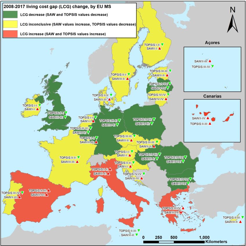
Figure 5.5. Change
Figure ChangeofofLCG
LCG (2008–2017)
(2008–2017) across
across the the EU Map
EU MS. MS. Map
labelslabels with Roman
with Roman style numerals
style numerals display
display
SAW and SAW and quartile
TOPSIS TOPSIS values
quartileforvalues forthe
2008 in 2008
leftin thefor
and left andatfor
2017 the2017
rightatside
theof
right side of the
the hyphen (-).
hyphen (-).
Quartile Quartile
I–means I–means
the lowest LCGthewhile
lowest LCG while
quartile quartile
IV means IV means
the highest LCG. the highest
Red arrows LCG. Redincrease
N show arrows
▲ show
and greenincrease
arrowsHand green
show arrows▼
decrease show
of both SAWdecrease of bothvalues
and TOPSIS SAW and(LCG)TOPSIS
in 2017values (LCG)toin2008.
compared 2017
compared to 2008.
At the other end, i.e., the group of MS where the LCG clearly expanded over the period 2008–
2017, landed Greece, Italy, and Spain, the countries that were hit maybe the most by the financialSustainability 2020, 12, 8955 12 of 26
At the other end, i.e., the group of MS where the LCG clearly expanded over the period 2008–2017,
landed Greece, Italy, and Spain, the countries that were hit maybe the most by the financial and
economic crisis in 2008–2009. The LCG values from Figures 2 and 3 suggest that the LCG expansion
was the most pronounced in Spain, which shifted from the second (moderate LCG) quartile in 2008
to the third (high LCG) and the even fourth (very high LCG) quartile in 2017. Spain was followed
by Greece that descended from the third (high LCG) quartile in 2008 to the fourth (very high LCG)
quartile in 2017. Amongst those three MS, Italy was the least affected by the downward trend in LCG,
because the LCG levels were relatively low in both 2008 and 2017 and hence, in 2017 the country firmly
landed in the second (moderate LCG) quartile.
4.4. The LCG Roots
The calculations showed that the objective criteria importance did not change much over the
years, considering that input data distributions remained uniform/constant (Table A3). The indicator
on household savings turned out to be the most important one (qi = 0.036) for LCG (Table A3) during
the period 2008–2017. This is because household savings criterion values were the most scattered [66]
compared to the other criteria values included in the LCG assessment.
During the 2008–2011 period, the immigration criterion was equally important (qi = 0.036) as
household saving. The importance of immigration in that period was higher compared to the one
in the following period 2011–2017. The objective function on immigration was set to minimisation,
i.e., we looked for the MS with the lowest immigration rates. The reasoning of this objective function
suggested (Table A2) that the economic situation in MS (to host the migrants) was tough and migrants
(especially the economic ones) could not earn decent income and savings (Table A2). The high initial
importance of that criteria could be possibly explained by the financial and economic crisis of 2008–2009
and the following recovery in the MS, which had little to offer to the migrants, especially to the
economic ones. Consequently, the criterion indicated higher LCG, but it did not explain the driving
reasons behind.
Indicators of relatively lower importance (medium scattering) were revealed: net household
income, GDP, remittances, migration (except, as already explained, the migration in the
initial period 2008–2011), imports, and optional household expenses on education, restaurants,
and miscellaneous goods.
Least important (least scattered) criteria were identified: exports, low work intensity, risk of
income poverty, unemployment, tenure status, and household expenditure on other needs (besides
education, restaurants, and miscellaneous goods) Table A3.
In order to comprehensively address the LCG, we introduced all indicators (Table A3) and their
importance into multi-criteria analyses.
4.5. LCG Drivers
We did not aim to measure income inequality [67], poverty [68,69], the households’ quality of
life [70], or other phenomenon describing social and economic well-being [71] across the MS. The goal
of the composite multidimensional LCG indicator was to identify core criteria impacting living cost
gap across the MS. This indicator shows how large/small the living cost gap is (distance wise), but it
does not explain how good or bad the living cost situation is.
Following our results, SAW and TOPSIS outcomes suggested that ranking results (Tables A4 and A5)
were ambiguous and inconclusive for the second and third quartiles (Figure 5). The correlation
between CAGRs of SAW and TOPSIS values was moderate (r = 0.72) and thus, it could be considered
as moderately reliable for the highest (fourth quartile) and lowest (first quartile) ranks (Figure 5) where
both methods had shown the same results.Sustainability 2020, 12, 8955 13 of 26
In order to understand how criteria changes were relating with LCG change across MS, we analysed
the relationship between CAGR [56] of each indicator with CAGRs of SAW (Table A4) and TOPSIS
(Table A5). The CAGR is defined as:
!t 1
V ( tn ) n −t0
CAGR (t0 , tn ) = −1 (1)
V ( t0 )
Sustainability 2020, 12, x FOR PEER REVIEW 14 of 29
where V(t0 ) is the initial value, V(tn ) is the end value, and tn −t0 is the number of years. The actual
wherehave
values V(t0)been
is theused
initial
for value, V(tn) is the end value, and tn-t0 is the number of years. The actual
calculations.
values
Thehave
value been
of rused for calculations.
(Pearson correlation index) lies between (−1) and (1), inclusive (Figure 6). That is,
The value of r (Pearson
–1 ≤ r ≤ 1. If r took positive value, correlation index) lies
the variables between
were (−1) and
positively (1), inclusive
correlated. (Figure
If r took 6). That
negative is,
value,
–1 ≤ r ≤ 1. If r took positive value, the variables were positively correlated. If r took
the variables were negatively correlated. If r took the value 0, then there was no relationship between negative value,
theCAGRs
the variables were negatively
of indicators and CAGRs correlated. If r TOPSIS
of SAW and took the(LCG).
valueIn0,our
then there
study, we was
usedno relationshipof
interpretation
r between
as: 0–no the CAGRs 0oftoindicators
association; 0.25 (0 to and CAGRs ofassociation;
−0.25)—weak SAW and TOPSIS (LCG).
0.25 to 0.50 In our
(−0.25 study, we used
to −0.50)—moderate
interpretation of r as: 0–no association; 0 to 0.25 (0 to −0.25)—weak association;
association; 0.50–0.75 (−0.50 to −0.75)—strong association; 0.75 to 1.00 (−0.75 to −1.00)—very 0.25 to 0.50 (−0.25 to
strong
−0.50)—moderate association; 0.50–0.75
association; and 1 (−1)—perfect association [72]. (−0.50 to −0.75)—strong association; 0.75 to 1.00 (−0.75 to
−1.00)—very strong association; and 1 (−1)—perfect association [72].
Figure6.6.Pearson
Figure Pearsoncorrelation
correlationvalues
valuesbetween
betweenCAGR
CAGR ofof each
each indicator
indicator and
and CAGRs
CAGRs of SAW
of SAW (Table
(Table A4)A4)
and
and TOPSIS
TOPSIS (Table(Table A5), across
A5), across all MSall MS (Table
(Table A6). lines
A6). Black Blackillustrate
lines illustrate distances
distances between
between correlation
correlation values.
values.
The relationship (Pearson correlation coefficient) between SAW and TOPSIS CAGRs values was
(r =
strongThe relationship
0.72) which (Pearson correlation
re-confirmed coefficient)
the that betweenshowed
both methods SAW and TOPSIS
the same CAGRs values
trends (not was
perfect,
strong
but (r = 0.72)
reliable) which
of LCG re-confirmed
across MS. Pearson thecorrelation
that both methods showed
coefficients the samethe
also revealed trends (not perfect,
relationship but
between
reliable)ofofSAW
CAGRs LCGandacross MS. with
TOPSIS Pearson correlation
CAGRs coefficients
of all criteria (Figurealso
6).revealed
Negativethe relationship
coefficient between
values meant
CAGRs of
opposite SAW and
trends, i.e., TOPSIS
increased with CAGRs
values of all
in one criteria
array and(Figure 6). Negative
decreased in anothercoefficient values meant
one. Positive values
opposite parallel
indicated trends, i.e., increased
trends, i.e., thevalues
valuesin in
oneeither
arrayarrays
and decreased
increasedinoranother
decreased one.atPositive
the samevalues
time.
indicated parallel trends, i.e., the values in either arrays
Simultaneous growth of SAW and TOPSIS values predisposed escalating LCG. increased or decreased at the same time.
Simultaneous growth
The correlation of SAW(Figure
analyses and TOPSIS values revealed
6) of CAGRs predisposedthatescalating
CAGR of LCG LCG.grew when CAGRs of
The correlation analyses
the following indicators across MS rose:(Figure 6) of CAGRs revealed that CAGR of LCG grew when CAGRs
of the following indicators across MS rose:
• With strong positive relationship: unemployment and low work intensity;
• With moderate positive relationship: housing cost overburden and basic household
expenditures, i.e., food, housing;
• With weak positive relationship: house tenants, risk of income poverty, exports, and optionalSustainability 2020, 12, 8955 14 of 26
• With strong positive relationship: unemployment and low work intensity;
• With moderate positive relationship: housing cost overburden and basic household expenditures,
i.e., food, housing;
• With weak positive relationship: house tenants, risk of income poverty, exports, and optional
household expenditures (alcoholic beverages, tobacco).
The correlation analyses of CAGR s revealed that CAGR of LCG expanded when CAGRs of
following indicators across all MS decreased:
• With strong negative relationship: GDP (in line with [66]), all types of net household earnings,
household expenditure on optional needs (furnishing and clothing);
• With moderate negative relationship: immigration, remittance flows, home ownership, optional
household expenditures (recreation and miscellaneous);
• With weak negative relationship: household savings, imports, optional household expenditures
(communications, education, transport, restaurants, and health).
Household income and expenditures constantly increased across the large majority of MS within
2008–2017. There was, however, a strong negative relationship (correlation) between LCG and
household income. In order to shrink LCG (in the countries where TOPSIS and SAW values were
the highest) it is necessary to focus on balancing “income and wealth effects” [66,73,74], increasing
household saving rate and directing savings to support household basic needs rather than onto
acquisition of financial and/or non-financial assets, i.e., converting them into “investment vehicles” [75].
4.6. LCG and Housing
The notion “Housing” can be defined as differential amongst tenure type, housing cost/affordability,
crowding, and quality [7,76,77]. Our study shows that the largest expenditure of the average households
was on housing and amounted to more than 20% of the net household income during the period
2008–2017 (Table A1). More specifically, the average net household expenditures on housing was
~21.0% in 2008 and ~21.8% in 2017 (with the highest peak of 22.7% in 2013) across the MS. The highest
(in the range of 25–30%) average household expenditure on housing was observed in Czechia, Denmark,
France, Slovakia, Finland, Sweden, and the United Kingdom. At the other end, the lowest (in the range
of 10–20%) average household expenditure on housing was recorded in Bulgaria, Estonia, Croatia,
Cyprus, Lithuania, Malta, Portugal, and Slovenia. The largest decrease (CAGR 2008–2017) in household
expenditures on housing occurred in Malta, Cyprus, Hungary, and Germany, while an increase was
registered for Finland, Portugal, Netherlands, Bulgaria, Spain, and Luxembourg (Table A6).
The CAGR of household expenditure on housing (2008–2017) tended to slightly increase in parallel
with the rise in CAGR of unemployment, low work intensity, risk of income poverty, housing cost
overburden, home rentals, savings, food, health, and remittance inflows. The CAGR of household
expenditure on housing tended to decrease with the growth in CAGR of household expenditure on
optional needs (except health), transport, net income, home ownership, trade, migration, and GDP
remittance outflows (Table A6).
Based on the above findings, we can conclude that household expenditure on housing increased
when household expenditure on other basic needs also grew, while household expenditure on housing
shrunk when household income and expenditure on optional needs grew. In the MS where household
net income was higher (e.g., Luxembourg, the Netherlands, Germany Sweden, the United Kingdom,
Denmark, Belgium), the rest of household expenses (after expenses on housing) were dedicated to
optional needs and savings. In the MS where household net income was lower (e.g., Lithuania, Bulgaria,
Romania, Latvia, Hungary, Poland, Croatia, Czechia, Estonia), the rest of household expenses were
dedicated to basic needs without (e.g., in the case of Lithuania, Latvia, Bulgaria,) or with minimum
savings (Table A6).Sustainability 2020, 12, 8955 15 of 26
Ultimately, the CAGR of housing cost overburden rate had a positive moderate (SAW) to
strong (TOPSIS) relationship (Table A6) with CAGR of SAW and TOPSIS values (LCG indicator).
This is a logical conclusion that re-confirms the reliability of the so-obtained LCG ranking results.
When confronted with housing cost overburden, households can adapt by reducing their housing
consumption via accepting smaller space and lower quality standards [7,78].
5. Conclusions
The LCG describes the difference between the income that households earn and what they need
to live. Household net income slowly but constantly increased in the majority of MS within 2008–2017.
In most cases, the household expenditures also increased and hence, the relatively scattered household
savings did not change significantly during the same period of time.
LCG was more prevalent in those MS where households were exposed to higher levels of
unemployment, low work intensity, higher housing cost overburden, and higher expenditures on basic
needs. Our research highlights the needs to mitigate unemployment and low household net income to
narrow LCG across the MS.
Increasing household expenditures on basic needs (food, housing, and transport) in households
with lower net income brought rise in LCG. The highest LCGs were found in those MS where household
incomes were the lowest. The LCG was lower in those MS where GDP, immigration, household income,
and household expenditure on optional needs and home ownership were higher.
Income and expenses constantly increased across all MS from 2008–2017. There was, however,
a moderate relationship between LCG and household income.
In order to narrow LCG in those countries where LCG were the highest, it is necessary to
significantly increase household income and income options, while at the same time look for reserves
to boost household savings. Poorer households cannot, however, benefit much from negligible income
growths due to the parallel rise in living costs.
Conversely, in order to maintain low or even decreasing LCG, it might be useful to upkeep
constant growth of household net income and household savings.
The elaborated methodology might be applied to mitigating LCG by employing also other
social-economic criteria at different spatial-temporal scales. Further research might include more
high-resolution data to refine the LCG estimates at higher spatial scale such as: cities, towns, suburbs,
and even–rural areas.
Author Contributions: Conceptualization, A.K.; methodology, A.K. and B.K.; software, A.K.; validation, A.K.;
formal analysis, B.K.; investigation, B.K.; resources, C.L.; data curation, A.K.; writing—original draft preparation,
A.K.; writing—review and editing, B.K.; visualization, A.K.; supervision, C.L.; project administration, C.L.;
funding acquisition, C.L. All authors have read and agreed to the published version of the manuscript.
Funding: This research received no external funding.
Acknowledgments: The authors would like to sincerely thank to Carolina Perpiña Castillo, Paola Proietti,
Jean-Philippe Aurambout and Filipe Batista e Silva for their thorough comments and helpful suggestions that
have resulted in a much-improved version of this manuscript.
Conflicts of Interest: The authors declare no conflict of interest.
Disclaimer: Responsibility for the information and views set out in this paper lies entirely with the authors.
More specifically, the scientific output expressed does not imply a policy position of the European Commission.
Neither the European Commission nor any person acting on behalf of the Commission is responsible for the use
that might be made of this publication.Sustainability 2020, 12, 8955 16 of 26
Appendix A
Table A1. Eurostat and World Bank data (2008–2017) metadata.
No. Indicator/Criterion Name 1 Unit of Measure Brief Description
1. Food and non-alcoholic beverages
2. Alcoholic beverages, tobacco, and narcotics
3. Clothing and footwear
4. Housing, water, electricity, gas, and other fuels
Furnishings, household equipment and Household expenditure refers to any spending done by a person living alone or by a group of
5.
routine household maintenance people living together in shared accommodation and with common domestic expenses.
6. Health Percentage of total household It includes expenditure incurred on the domestic territory (by residents and non-residents) for
expenditure the direct satisfaction of individual needs and covers the purchase of goods and services,
7. Transport the consumption of own production (such as garden produce) and the imputed rent of
8. Communications owner-occupied dwellings [41].
9. Recreation and culture
10. Education
11. Restaurants and hotels
12. Miscellaneous goods and services
The gross saving rate of households (including Non-Profit Institutions Serving Households) is
defined as gross saving divided by gross disposable income, with the latter being adjusted for
13. Household savings Saving percentage per household
the change in the net equity of households in pension funds reserves. Gross saving is the part of
the gross disposable income which is not spent as final consumption expenditure [42].
Annual net earnings of single person without Information on net earnings (net pay taken home, in absolute figures) and related tax-benefit
14. Total EUR per capita
children rates (in%) complements gross-earnings data with respect to disposable earnings. The transition
Annual net earnings of married couple with from gross to net earnings requires the deduction of income taxes and employee’s social security
15.
no children Total EUR per household contributions from the gross amounts and the addition of family allowances, if appropriate [43].
Annual net earnings of married couple with
16.
two children
Percentage of the population living in a household where total housing costs (net of housing
17. Housing cost overburden rate Percentage of total population allowances) represent more than 40% of the total disposable household income (net of housing
allowances) [44].
18. Tenants, 18 yo and older Distribution of population by a broad group of citizenship and tenure status (population aged 18
Percentage of total population
and over) [45].
19. Homeowners, 18 yo and olderSustainability 2020, 12, 8955 17 of 26
Table A1. Cont.
No. Indicator/Criterion Name 1 Unit of Measure Brief Description
The indicator is calculated as the ratio of real GDP to the average population of a specific year.
GDP measures the value of total final output of goods and services produced by an economy
within a certain period of time. It includes goods and services that have markets (or which could
Gross domestic product (GDP) at market have markets) and products which are produced by general government and non-profit
21. Total EUR per capita
prices institutions. It is a measure of economic activity and is also used as a proxy for the development
in a country’s material living standards. However, it is a limited measure of economic welfare.
For example, GDP does not include most unpaid household work nor does GDP take account of
negative effects of economic activity, like environmental degradation [47].
People living in households with very low work intensity are people aged 0–59 living in
22. Households with very low work intensity Percentage of total population households where the adults work 20% or less of their total work potential during the past year
[48].
People at risk-of-poverty are persons with an equivalised disposable income below the
23. People at risk of poverty rate Percentage of total population risk-of-poverty threshold, which is set at 60% of the national median equivalised disposable
income (after social transfers). The indicator is part of the multidimensional poverty index [49].
24. Remittance inflows 1 World Bank staff calculation based on data from IMF Balance of Payments Statistics database and
Total USD per capita
data releases from central banks, national statistical agencies, and World Bank country desks [54].
25. Remittance outflows 1
Total number of long-term emigrants leaving from the reporting country during the reference
26. Emigration
Percentage of total population year [50].
Total number of long-term immigrants arriving into the reporting country during the reference
27. Immigration
year [51].
This indicator is the value of exports of goods and services divided by the GDP in current prices
28. Exports of goods and services
Percentage of GDP [52].
This indicator is the value of imports of goods and services divided by the GDP in current prices
29. Imports of goods and services
[53].
The unemployment rate is the number of unemployed persons as a percentage of the labour
force based on International Labour Office (ILO) definition. The labour force is the total number
of people employed and unemployed. Unemployed persons comprise persons aged 15 to 74
20. Unemployment rate, aged 15–74 Percentage of active population
who are without work during the reference week, are available to start work within the next two
weeks, and have been actively seeking work in the past four weeks or had already found a job to
start within the next three months [46].
1 World Bank data.Sustainability 2020, 12, 8955 18 of 26
Table A2. Objective function description addressing the LCG.
Criterion No. 1 Objective Function Group Objective Function (Focusing on Highest LCG) Explanation Objective Function Defined
1 ii. Adjacent–Micro–Local–Individual Household expenditure on food (basic needs) is the highest. MAX
2 iii. Adjacent–Micro–Local–Individual Household expenditure on alcoholic beverages (optional needs) is the lowest. MIN
3 iii. Adjacent–Micro–Local–Individual Household expenditure on clothing (optional needs) is the lowest. MIN
4 ii. Adjacent–Micro–Local–Individual Household expenditure on housing (basic needs) is the highest. MAX
5 iii. Adjacent–Micro–Local–Individual Household expenditure on furniture (optional needs) is the lowest. MIN
6 iii. Adjacent–Micro–Local–Individual Household expenditure on health (optional needs) is the lowest. MIN
7 ii. Adjacent–Micro–Local–Individual Household expenditure on transport (basic needs) is the highest. MAX
8 iii. Adjacent–Micro–Local–Individual Household expenditure on communications (optional needs) is the lowest. MIN
9 iii. Adjacent–Micro–Local–Individual Household expenditure on recreation (optional needs) is the lowest. MIN
10 iii. Adjacent–Micro–Local–Individual Household expenditure on education (optional needs) is the lowest. MIN
11 iii. Adjacent–Micro–Local–Individual Household expenditure on restaurants (optional needs) is the lowest. MIN
12 iii. Adjacent–Micro–Local–Individual Household expenditure on miscellaneous goods (optional needs) is the lowest. MIN
Household savings are the lowest. Smallest savings means that most of income is spent on basic needs. This is
13 i. Adjacent–Micro–Local–Individual MIN
the major driver of economic emigration.
Single person income is the smallest. Smallest net income means that less money for optional expenditures and
14 i. Adjacent–Micro–Local–Individual MIN
savings.
Family without children income is the smallest. Smallest net income means that less money for optional
15 i. Adjacent–Micro–Local–Individual MIN
expenditures and savings.
Family with children income is the smallest. Smallest net income means that less money for optional
16 i. Adjacent–Micro–Local–Individual MIN
expenditures and savings.
Household cost overburden rate is highest. Means that less money households can allocate for optional
17 v. Neighboring–Mezo–National–External MAX
expenditures and savings.
Tenant ratio is the highest. Means competition for the housing is higher. It also means that less money
18 v. Neighboring–Mezo–National–External MAX
households can allocate for optional expenditures and savings.
Homeowner ratio is the smallest. Means competition for the housing is smaller. It also means that more money
19 v. Neighboring–Mezo–National–External MIN
households can allocate for optional expenditures and savings.
Unemployment rate is the highest. Means that competition for workplaces is high. It also means that household
20 iv. Neighboring–Mezo–National–External MAX
receive less income and have to allocate larger share of income for basic needs.
GDP is lowest. Low GDP show low country economic performance. It means that more money households
21 iv. Neighboring–Mezo–National–External MIN
have to spend on basic needs.
22 iv. Neighboring–Mezo–National–External The low work intensity is the highest. It also means lower income for the households. MAX
The highest number of population within the income poverty. It means that largest share of household income
23 iv. Neighboring–Mezo–National–External MAX
is allocated only for the basic needs.
The remittance inflows are highest. It also shows that economic and employment situation in the country is
24 vi. Distant–Macro–International–External MAX
tough because incoming remittances are used to support basic local household needs.
The remittance outflows are lowest. It also shows that economic and employment situation in the country is
25 vi. Distant–Macro–International–External MIN
tough because the low outgoing remittances show that there is no possibility to earn decent savings.
26 vi. Distant–Macro–International–External The emigration is the highest. It shows that most of household income share are allocated for the basic needs. MAX
The immigration is the lowest. It shows that economic situation in country is tough and immigrants (especially
27 vi. Distant–Macro–International–External MIN
economic ones) cannot earn decent income and savings.
The export is the lowest. No production, no export of goods, no import of money. It also means that households
28 vi. Distant–Macro–International–External MIN
in such country have to allocate more money for basic needs because of lower income.
The import is the highest. No production, so import of goods and export of money. It also means that
29 vi. Distant–Macro–International–External MAX
households in such country have to allocate more money for basic needs because of lower income.
1 Table A1.You can also read