Comparing Deep-Learning Architectures and Traditional Machine-Learning Approaches for Satire Identification in Spanish Tweets - MDPI
←
→
Page content transcription
If your browser does not render page correctly, please read the page content below

mathematics
Article
Comparing Deep-Learning Architectures and
Traditional Machine-Learning Approaches for Satire
Identification in Spanish Tweets
Óscar Apolinario-Arzube 1,† , José Antonio García-Díaz 2,† , José Medina-Moreira 3 ,
Harry Luna-Aveiga 1 and Rafael Valencia-García 2, *
 1   Facultad de Ciencias Matemáticas y Físicas, Universidad de Guayaquil, Cdla, Universitaria Salvador
     Allende, Guayaquil 090514, Ecuador; oscar.apolinarioa@ug.edu.ec (Ó.A.-A.);
     harry.lunaa@ug.edu.ec (H.L.-A.)
 2   Facultad de Informática, Universidad de Murcia, Campus de Espinardo, 30100 Murcia, Spain;
     joseantonio.garcia8@um.es
 3   Facultad de Ciencias Agrarias, Universidad Agraria del Ecuador, Av. 25 de Julio,
     Guayaquil 090114, Ecuador; jmedina@uagraria.edu.ec
 *   Correspondence: valencia@um.es
 †   These authors contributed equally to this work.

 Received: 27 October 2020; Accepted: 17 November 2020; Published: 20 November 2020

 Abstract: Automatic satire identification can help to identify texts in which the intended meaning
 differs from the literal meaning, improving tasks such as sentiment analysis, fake news detection
 or natural-language user interfaces. Typically, satire identification is performed by training a
 supervised classifier for finding linguistic clues that can determine whether a text is satirical or
 not. For this, the state-of-the-art relies on neural networks fed with word embeddings that are
 capable of learning interesting characteristics regarding the way humans communicate. However,
 as far as our knowledge goes, there are no comprehensive studies that evaluate these techniques
 in Spanish in the satire identification domain. Consequently, in this work we evaluate several
 deep-learning architectures with Spanish pre-trained word-embeddings and compare the results with
 strong baselines based on term-counting features. This evaluation is performed with two datasets
 that contain satirical and non-satirical tweets written in two Spanish variants: European Spanish
 and Mexican Spanish. Our experimentation revealed that term-counting features achieved similar
 results to deep-learning approaches based on word-embeddings, both outperforming previous
 results based on linguistic features. Our results suggest that term-counting features and traditional
 machine learning models provide competitive results regarding automatic satire identification,
 slightly outperforming state-of-the-art models.

 Keywords: automatic satire identification; text classification; natural language processing

1. Introduction
     Satire is a literary genre in which individual or collective vices, follies, abuses, or deficiencies are
revealed through ridicule, farce, or irony [1]. The history of universal literature is full of writers who
have practised satire with great skill and well-known works such as Don Quijote de la Mancha, (1605) by
Miguel de Cervantes, The Life of Lazarillo de Tormes and of His Fortunes and Adversities (1554) of unknown
authorship, The Swindler (1626) by Francisco de Quevedo, Gulliver’s travels (1726) by Jonathan Swift,
Animal Farm (1945) by George Orwell, or Brave New World (1932) by Aldous Huxley.
     According to the Merriam-Webster Dictionary (https://www.merriam-webster.com/dictionary/
satire), satire is defined as “a way of using humour to show that someone or something is foolish, weak, bad,

Mathematics 2020, 8, 2075; doi:10.3390/math8112075                         www.mdpi.com/journal/mathematics
Mathematics 2020, 8, 2075                                                                                2 of 23

etc." and “humour that shows the weaknesses or bad qualities of a person, government, society, etc.". From these
two definitions we can assume that in satire everything is devised with a critical and constructive spirit
to achieve a better society. The funny and interesting combination of humour and critique has led
certain journalists to create satirical news websites, such as The Onion (https://www.theonion.com/),
that have gained popularity by publishing news imitating the style of mainstream journalism with
the aim of social criticism with a sharp sense of humour [2,3]. However, satiric news press is often
confused with fake news because both present untrue news but with opposite objectives: whereas
satire has a moralising purpose, the aim of fake news is deception and misleading [4]. In a broad
sense, deception content in news media can be present in different manners. There are, for example,
articles that express outrage towards someone or something, others that provide a true event but
then make some false interpretations and even articles that contain pseudo-scientific content. Some
other articles are really only an opinion disguised as news, or articles with a moralising purpose.
Consequently, automatic satire identification has also gained attention in order to develop better
fake news detectors capable of distinguishing among false and misleading content from playful and
burlesque news.
      Satirical writers employed linguistic devices typical from figurative language, such as irony,
sarcasm, parody, mockery, exaggeration or opposing two issues that are very different from each other
to devalue one and give greater importance to the other making comparisons, analogies or folds [5].
Satire offers the readers a complex puzzle to be untangled until the final twist is revealed. That is
the reason that satire is so inherently ambiguous and difficult to grasp its true intentions, even for
humans [6]. The requirement of strong cognitive abilities hinders some Natural Language Processing
(NLP) text classification tasks, such as sentiment analysis, fake news detectors, natural-language user
interfaces or review summarisation [7]. However, it is necessary to get around this difficulty in order
to develop better interfaces based on natural language, capable of identifying the real intentions of the
communication, or better sentiment analysis tools, capable of finding ironic utterances that can flip the
real sentiment from a product review, or make better summaries that identify what the true intention
of the writer was.
      In the last decade, the approaches for conducting automatic satire identification has evolved
from traditional machine-learning methods for finding linguistic and stylometric features on the
texts to modern deep-learning architectures such as convolutional and recurrent neural networks fed
with word-embeddings that allows to represent words and other linguistic units by incorporating
co-occurrence properties of the human language [8]. Although the majority of NLP resources are
focused on the English language, scientific research is making great efforts to adapt these technologies
to other languages like Spanish. One of the most outstanding contributions in this regard is the
adaptation of some of the state-of-the-art resources to Spanish [9]. These new resources are being used
for evaluating some NLP tasks such as the work described in [10], focused on hate speech detection in
social networks in Spanish.
      As far as our knowledge goes, these new pre-trained word embeddings have not yet been
employed in automatic satire identification. It is important to remark that Spanish is different from
English in many aspects. The order between nouns and adjectives, for example, is reversed compared
to English. Spanish makes an intensive use of inflection to denote gender and number and it requires
an agreement between nouns, verbs, adjectives or articles. Moreover, the number of verb tenses is
higher in Spanish than in English. We consider that these differences are relevant, as word embeddings
learn their vectors from unsupervised tasks such as next-word prediction or word analogy. Therefore,
we consider than the next step is the evaluation of these new NLP resources in tasks regarding
figurative language, such as satire identification.
      Consequently, in this paper we evaluate (1) four supervised machine-learning classifiers trained
with term-counting features that are used as a strong baseline, and (2) four deep-learning architectures
combined with three pre-trained word embeddings. To compare these models, we use two datasets
composed of tweets written in European Spanish and Mexican Spanish. The underlying goal for
Mathematics 2020, 8, 2075                                                                            3 of 23

this work is to determine what kind of features and architectures increase the results for developing
automatic satire classifiers focused in Spanish. The findings in these kinds of systems will allow to
improve NLP tools by distinguishing between texts in which the figurative meaning differs from their
literal meaning. In addition, as we compare traits from two datasets of the same language but different
zones and linguistic variants, we investigate if cultural and background differences are relevant for
satire identification in Spanish.
      The rest of the document is organised as follows. Section 2 contains background information about
text classification approaches and satire identification in the bibliography and workshops. Section 3
describes the materials and methods used in our proposal, including the dataset, the supervised
classifiers, deep-learning architectures and the pre-trained word embeddings. Then, the results
achieved are shown in Section 4 and analysed in detail in Section 5. Finally, in Section 6 we summarise
our contributions and propose new research lines for improvement regarding satire classification.

2. Background Information
     In this work, different feature extraction methods and different supervised machine and
deep-learning classifiers for solving satire identification are evaluated. Consequently, we provide
background information regarding text classification (see Section 2.1) and we analysed previous
research that deals with the identification of satire (see Section 2.2).

2.1. Text Classification Approaches
      NLP is one of the fundamental pillars of Artificial Intelligence (AI). It is based on the
interface between human language and their manipulation by a machine. NLP come into play
in understanding language to design systems that perform complex linguistic tasks such as translation,
text summarisation, or Information Retrieval (IR) among others. The main difficulty in IR processes
through natural languages is, however, not technical, but psychological: understanding what the user’s
real needs are or what is the correct intention of the question they asked. Automatic satire identification
belongs to the NLP’s task known as automated text classification, which consists of the categorisation
of a certain piece of text with one or more categories, usually from a predefined set. Text classification
relies heavily on IR and Machine Learning (ML), based on supervised or semi-supervised classification
in which the models are learned from a labelled set used as examples [11].
      There are different models that can be used for representing natural language data to perform
automatic text classification, some of them discussed in different surveys such as [12,13]. The main idea
for text classification is to extract meaningful features that represent data encoded as natural language.
There are different approaches for doing this, and, naturally, all of them have their own benefits and
drawbacks. For example, old-school techniques based on term-counting are the Bag of Words (BoW)
model and its variants (word n-grams or character n-grams). In these models, each document is
encoded as a vector of a fixed length based on the frequencies of their words and the automatic text
classifiers learn to discern between the documents based on the appearance and frequency on certain
words. Although these techniques are surprisingly effective [14], these models have serious limitations.
The most important one is that term-counting features do not consider neither the context nor the
word order. This over-simplification causes many of the nuances of human communication to be lost.
Some phenomena, such as homonymy, synonymy or polysemy, make it almost impossible to get their
meaning if we do not know the context of the conversation. Another drawback is that all words are
equally distributed in term-counting based approaches. That means that, conceptually, there is the
same relationship between the words dog, cat, and microphone. So, the resulting models are closely
tied to training data but can fail with unseen data. Distributional models such as word embeddings
can solve these limitations by representing words as dense vectors, in which the basic idea is that
similar terms tend to have similar representations. Word embeddings provide more robust models
that can predict unseen sentences but with similar words to the ones used during training. Another
improvement for text classification is the usage of deep-learning architectures, such as convolutional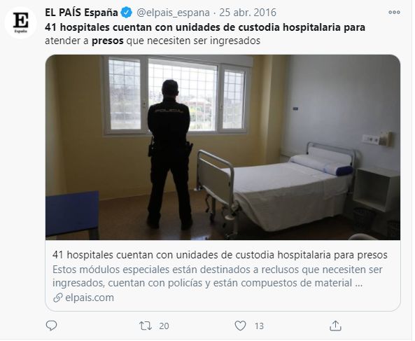
Mathematics 2020, 8, 2075                                                                               4 of 23

or recurrent neural networks, that are capable of understanding the spatial and temporal dimension of
the natural language; that is, the order in which the words are said, and how to identify joint words
that represent complex ideas than the words that form those joint words [15].

2.2. Satire Identification
      In this section we analyse in detail recent works concerning automatic satire identification as well
as shared tasks regarding irony classification, which is a figurative device proper from satire. Due to
the scope of our proposal, we explore works mainly focused on Spanish. However, we also include
other works in English, because it is the language that has the most PLN resources, and a few of the
works focused on other languages that we consider relevant for our study.
      As satire is a literate genre, we investigate those works that consider linguistic and stylistic features
for satire identification. In the work described in [16], the authors identified key value components
and characteristics for automatic satire detection. They evaluated those features from several datasets
written in English including tweets, product reviews, and news articles. They combined (1) baseline
features based on word n-grams; (2) lexical features from different lexicons; (3) sentiment amplifiers
that include quotations, certain punctuation rules, and certain emoticons; (4) speech act features with
apologies, appreciations, statements, and questions; (5) sensorial lexicons related to the five basic
senses; (6) sentiment continuity disruption features that measures sentiment variations in the same
text; and (7) specific literary device features, such as hyperbole, onomatopoeia, alliterations, or imagery.
Their best results were achieved with an ensemble method that combined traditional machine learning
classifiers, such as Random Forest, Logistic Regression, Support Vector Machines and Decision Trees.
Another work regarding satire identification in English is described in [17], in which the authors
proposed a system capable of detecting satire, sarcasm and irony from news and customer reviews.
This system was grounded on assembled text feature selection. The effectiveness of their proposal
was demonstrated in three data sets, including two satirical and one ironic. During their research,
the authors discovered some interesting common features of satire and irony such as affecting process
(negative emotion), personal concern (leisure), biological process (bodily and sexual), perception (see),
informal language (swear), social process (masculine), cognitive (true), and psycho-linguistic processes
(concretion and imagination), which were of particular importance. In [18], the authors presented a
method for the automatic detection of double meaning of texts in English from social networks. For the
purposes of this article, they defined double meaning as one of irony, sarcasm, and satire. They scored
six features and evaluated their predictive accuracy with three different machine learning classifiers:
Naive Bayes, k-Nearest Neighbours, and Support Vector Machines.
      In [19], the authors evaluated the automatic detection of tweets that advertise satirical news in
English, Spanish and Italian. To this end, the authors combined language-independent features that
describe the lexical, semantic, and word-use properties of each Tweet. They evaluated the performance
of their system by conducting monolingual and multilingual classification experiments, computing
the effectiveness of detecting satires. In [20], the authors proposed a method that employs a wide
variety of psycho-linguistic features that detects satirical and non-satirical tweets from a corpus
composed of tweets from satirical and non-satirical news accounts compiled from Mexico and Spain.
They used LIWC [21] for extracting psychological and linguistic traits from the corpus and use them
for evaluating three machine-learning classifiers. They achieved an F1-measure of 85.5% with the
Spanish Mexican dataset and an F1-measure of 84.0% with the European Spain dataset, both with
Support Vector Machines.
      Concerning other languages apart from English and Spanish, we can find some words regarding
satire identification. For example, in [22], the authors applied a hybrid technique to extract features
from text documents that merge Word2Vec and TF-IDF by applying a Convolutional Neuronal Network
for the deep-learning architecture, achieving an accuracy up to 96%. In [23], the authors presented a
machine learning classifier for detecting satires in Turkish news articles. They employed term-counting
based on the TF-IDF of unigrams, bigram and trigrams, and evaluated with some traditional
Mathematics 2020, 8, 2075 5 of 23
machine-learning classifiers such as Naïve Bayes, Support Vector Machines, Logistic Regression
and C4.5.
Satire identification plays a crucial role by discerning between fun and facts. In this sense, it is
possible to apply satire identification techniques in order to distinguish between satirical news and
fake news. In [24], for example, the authors performed an analytical study on the language of the
media in the context of the verification of political facts and the detection of fake news. They compared
the language of real news with that of satire, hoaxes and propaganda to find linguistic features of an
unreliable text. To evaluate the feasibility of automatic political fact checking, they also presented a
case study based on PolitiFact.com using their feasibility judgements on a six-point scale.
As satire identification is a challenging task that can improve other NLP tasks, the automatic
identification of satire and irony has been proposed in some workshops. Due to the scope of our
proposal, we highlight the forum for the evaluation of Iberian languages (IberLEF 2019), in which
a shared-task entitled “Overview of the task on irony detection in Spanish variants” [25] was proposed.
The participants of this shared task were asked to identify ironic utterances in different Spanish variants.
There was a total of 12 teams that participated in the task and the three best results achieved were an F1
macro average of 0.7167, 0.6803, and 0.6596, respectively. We analysed in detail some of the teams that
participated in the task. In [26], the authors trained a Linear Support Vector Machine with features that
capture morphology and dependency syntax information. Their approach achieved better results from
the European Spanish and Mexican Spanish datasets but slightly worse from the Cuban dataset. In [27],
the authors extracted term-counting features to feed a neural network. This proposal achieved the best
performance in the Cuban dataset and the second overall place in the shared task. Other proposals
were based on transformers. In [28], with a model based on Transformer Encoders and Spanish Twitter
embeddings learned from a large dataset compiled from Twitter. In [29], applying ELMo, and in [30],
using BERT. Other approaches focused on linguistic features. In [31], the authors presented stylistic,
lexical, and affective features. In [32], the approach was based on seven linguistic patterns crafted
from nine thousand texts written in three different linguistic variants. The linguistic patterns included
lists of laughter expressions, uppercase words, quotation marks, exclamatory sentences, as well as
lexicons composed of set phrases. The benefits of linguistic and affective features are that they provide
interpretable results that can be used for tracking analogies and differences in the expression of
irony. Finally, in [33], the author employed three different representations of textual information and
similarity measures using a weighted combination of these representations.
3. Materials and Methods
In a nutshell, our pipeline can be described as follows. First, we extract and pre-process a corpus
regarding satire identification in European Spanish and Mexican Spanish (see Section 3.1). We use
the training dataset to obtain term-counting features and embedding layers from pre-trained word
embeddings (see Section 3.2). Next, we use feature selection to obtain the best character and word
n-grams and we use them to train four machine-learning classifiers. Next, we use the embeddings
layer to feed four deep-learning architectures. All classifiers were fine-tuned performing a randomised
grid search for finding the best hyper-parameters and evaluating different deep-learning architectures.
Finally, we evaluate each model by predicting over the test dataset. This pipeline is depicted in Figure 1
and described in detail in the following sections.Mathematics 2020, 8, 2075 6 of 23
Figure 1. The pipeline of our proposal.
3.1. Data Acquisition
We identified the following datasets for conducting satire identification in Spanish: [20,34].
The corpus from [34] was compiled from Twitter and it is composed of tweets from news sites in
Spanish. However, the corpus was not available at the time we performed this work. In [20], the authors
conducted a similar approach from [34], but including satirical and non-satirical tweets compiled
from Twitter from Mexican Spanish news sites Twitter accounts. The final dataset contains tweets
from satiric media, such as El Mundo Today (https://www.elmundotoday.com/) or El Dizque (https:
//www.eldizque.com/) and traditional new sites such as El País (https://elpais.com/) or El Universal
(https://www.eluniversal.com.mx/). The resulting dataset was composed of 5000 satirical tweets in
which half of them were compiled from Mexico and the other half from Spain; and 5000 non-satirical
tweets with the same proportions. We could retrieve this corpus. However, according to the Twitter
guidelines, (https://developer.twitter.com/en/developer-terms/agreement-and-policy) this corpus
contains only the identifiers of the tweets to respect the rights of the users of the content. We use the
UMUCorpusClassifier tool [35] to retrieve the original dataset. Although some the tweets were not
available, we could retrieve 4821 tweets for the European Spanish dataset and 4956 tweets for the
Mexican Spanish dataset, which represent 96.42% and the 99.12% of the original dataset, respectively.
We divided each dataset into train, evaluation and test sets in a proportion of 60%-20%-20%.
We used the train and evaluation sets for training the models and evaluating the hyper-parameters,
and the test set for evaluating the final models. The details are explained in Section 3.5. The statistics
of the retrieved corpus are described in Table 1. In this sense, both datasets are almost balanced
with a slightly superior number of satirical tweets that it is more significant in the European Spanish
dataset (51.607% vs. 48.392%) than in the Mexican Spanish dataset (50.202% vs. 49.798%). It is
worth noting that the authors of this study performed a distant supervision approach based on the
hypothesis that all tweets compiled from satirical Twitter accounts can be considered as satirical and
those tweets compiled from non-satirical accounts can be considered safe. However, after a manual
revision of the corpus, we discovered some tweets labelled as satirical contain self-advertisements or
even non-satirical news. We decided to leave tweets as they were classified by the authors in order to
perform a fair comparison.
Each dataset contains tweets from four accounts: two satirical and two non-satirical. However,
as we can observe from Figure 2, these accounts are not balanced achieving an average of 1205.25
tweets per account with a standard deviation of 216.483 for the European Spanish dataset (see Figure 2
left) and an average of 1239 but with a standard deviation of 763.743 for the Mexican Spanish dataset
(see Figure 2 right). The high standard deviation of the Mexican Spanish dataset can cause overfitting,
over-weighting stylistic patterns of the predominant accounts (@eldeforma and @eluniversalmx) over the
full dataset.Mathematics 2020, 8, 2075 7 of 23
Table 1. Corpus statistics.
Feature-Set Tweets Satirical Non-Satirical
European Spanish 4821 2488 2333
train (60%) 2892 1493 1400
evaluation (20%) 964 497 466
test (20%) 965 498 467
Mexican Spanish 4956 2488 2468
train (60%) 2974 1493 1481
evaluation (20%) 991 497 493
test (20%) 991 498 494
Figures 3 and 4 contain four examples of a satirical and non-satirical tweet for both datasets.
In English, the translation are: 41 hospitals have hospital custody units for prisoners (see Figure 3 left),
Josep Guardiola insists on watering the grass of all European studios himself (see Figure 3 right), #Survey
#veracruz If today were the elections, there would be a technical tie between the #Yunes (see Figure 4 left),
and Incredible but true! ElDeforma collaborator trained #LadyMatemáticas (see Figure 4 right).
Figure 2. Corpus distribution per accounts for the European Spanish (left) and the Mexican Spanish
(right) datasets compiled in [20]. In red, satirical accounts. In green, non-satirical accounts.
Figure 3. Examples of non-satirical European Spanish (left) and satirical European Spanish
(right) tweets.Mathematics 2020, 8, 2075 8 of 23
Figure 4. Examples of non-satirical Mexican Spanish (left) and satirical Mexican Spanish (right) tweets.
Once the corpus was compiled, we performed a normalisation phase, which consisted of:
(1) removing blank lines and collapsing spaces and tabs. We also removed the intentional elongation of
some words that was used as an emphasising rhetorical device; (2) resolving some forms of informal
contractions that are popular in text-message medias, such as mñn into mañana (In English: tomorrow);
(3) removing hyperlinks and mentions; (4) encoding emoticons as textual forms (For example, :smile:)
in order to ease their identification; (5) fixing misspellings in the texts by using the ASPell library
(http://aspell.net/); and, finally, (6) transforming the texts into their lowercase form. Note that some
of these techniques was also conducted in the original experiment [20].
To automatically fix the misspellings, we split each tweet into words and checked if each word
did not start with an uppercase letter to prevent fixing proper names. Then, we used ASPell library for
checking if the word was well-written. If the word had misspellings, we looked for the suggestions list
and we replaced the misspelt word with its first suggestion if the distance [36] between the suggested
word and the original word was less or equal than 90% (this threshold was set by a trial-error method).
We followed this approach to have confidence that only obvious misspelt words were fixed.
3.2. Feature Extraction
The next step of our pipeline consisted of the extraction of the features to perform the supervised
classification. These features are organised into two major sets: (1) term-counting features, used with
the traditional machine-learning classifiers (see Section 3.2.1); and (2) word-embeddings, employed for
testing the deep-learning architectures (see Section 3.2.2).
3.2.1. Term-Counting Features
Term-counting features are the basis of the BoW model and its similar approaches. The objective
is the representation of natural language as vectors to facilitate computers and machine-learning
algorithms to deal with natural language. In BoW, each document is represented as a vector composed
of the frequency of their words. Typically, the vector size depends on all the words of the corpus, but it
is also possible to use specific domain lexicons to categorise the text according to some pre-established
domain. The pro of the BoW model is that it is easy to implement while it provides competitive results.
The BoW model has been employed as a strong baseline in text classification tasks for a long time.
However, the BoW model has some drawbacks. First, this model ignores completely the context of the
words. As each word is treated separately, the BoW model is weak against polysemy and synonymy.
The second drawback is that on large datasets and when the lexicon is composed of all the words in a
corpus, the resulting vectors are large and sparse, which causes a phenomenon known as the curse of
dimensionality, which hinders the ability of some machine-learning classifiers to learn at the same time
that increases time and memory requirements. The third drawback is that the BoW model tends to
over-represent some words based on the Zipf’s law, which states that words in both natural or artificial
languages follow long-range correlations [37]. Finally, the BoW model is not capable of handlingMathematics 2020, 8, 2075 9 of 23
unknown words, misspellings, and some popular ways of writing in social media that include the use
of abbreviations, slang and informal writing.
There are different approaches for solving the drawbacks of the BoW model. The word n-gram
model is an extension of the BoW model in which joint words (bigrams, trigrams) are considered.
Joint words have two major benefits: on the one hand, they can represent higher semantic concepts
than unigrams and, on the other, they can be used for word disambiguation. Another approach is
known as character n-grams, which consists of measuring characters instead of words. Character
n-grams are aware of misspellings or made-up words. Another improvement of the BoW model is the
application of the Term Frequency-Inverse Document Frequency (see Equation (1)) rather than raw
count frequencies. TF-IDF dismisses common words known as stop-words and highlights relevant
other keywords.
TFIDF = TF ∗ IDF (1)
TF = number_o f _occurrences/number_o f _grams (2)
IDF = log2 corpus_size/documents_with_terms (3)
3.2.2. Word Embeddings
As we have observed in Section 3.2.1, term-counting methods represent documents as frequencies
of tokens. In this sense, they ignore the position of each term in the sequence. In human communication,
however, the order of the words has a major impact on the meaning of the phrase. Negative clauses
and double negations, for example, can shift the meaning of a sentence depending on the words
they modify. On the other hand, term-counting models consider all words equal. That is, there is no
difference between terms neither on their syntactic, semantic or pragmatic function. These problems are
solved by using distributional models such as word embeddings, in which words are encoded as dense
vectors with the underlying idea that similar words have similar representation. Word embeddings
can be viewed as an extension of the one-hot encoding, which allows to represent categorical variables
as binary vectors. With one-hot encoding, words are encoded in fixed length vectors of the full
vocabulary, in which each vector has only one column with a value different to zero. In one-hot
encoding, therefore, each word is orthogonal with the rest of the words. With word embeddings,
however, the numeric representation of each vector is learned typically by training a neural network
with some general-purpose task, such as next-word prediction or word analogy. One of the major
benefits of word embeddings is that it is possible to learn those embeddings from large unannotated
datasets, such as social networks, news sites, or encyclopaedias among others, to obtain word vectors
that convey a general meaning that can be applied to solve other tasks faster.
Word embeddings have allowed the outperformance of several NLP tasks and have meant a
paradigm shift in NLP. In this sense, it is possible to use the same principles for encoding major
linguistic units such as sentences for creating sentence embeddings [38]. Other approaches have tried
to focus word-embeddings training for solving specific NLP tasks. For example, in [39], the authors
describe a method for learning word embeddings focused on sentiment analysis. The authors argue
that some of the techniques employed for learning word embeddings can cluster words with opposite
sentiments such as good or bad only because they have some similar syntactic function. They develop
neural networks that consider the sentiment polarity in the loss function and evaluated their approach
with some existing datasets focused on Sentiment Analysis.
In this paper, we focused on Spanish pre-trained word embeddings trained with different
approaches, including word2vec, fastText, and gloVe. These models and the resulting pre-trained
word-embeddings are described below.
• Word2Vec. Word2Vec was one of the firsts models for obtaining word embeddings.
With word2vec, word embeddings are learned by training a neural network, the objective of which
is next-word prediction [40]. Specifically, there are two methods for learning word-embeddings
with Word2Vec: (1) Continuous Bag of Words Model (CBOW), in which the objective is to predictMathematics 2020, 8, 2075 10 of 23
a word based on the context words; and (2) Skip-Grams, in which the objective is just the opposite:
predicting context words from a target word. Regardless of the approach, both strategies learn
the underlying word representations. The difference is that the CBOW model is faster as the
same time that provides better accuracy with frequent words and the Skip-Gram model is more
accurate using smaller training data at the same time that provides better representation of a
word that appears infrequently. The pre-trained word embeddings from Word2Vec used in this
experiment were trained with the Spanish Billion Corpora [41].
• GloVe. GloVe is a technique to learn with word embeddings that exploit statistical
information regarding word co-occurrences that is better suited for performing NLP tasks
such as word-analogy or entity recognition [42]. As the opposite of Word2Vec, where word
embeddings are learned applying raw co-occurrence probabilities, GloVe learns the ratio between
co-occurrences, which improves to learn fine-grained details in the relevance of two linked terms.
The pre-trained word embeddings from GloVe used in this work were trained with the Spanish
Billion Corpora [41].
• FastText. FastText is inspired in the word2vec model but it represents each word as a sequence
of character n-grams [43]. FastText is, therefore, aware of unknown words and misspellings.
In addition, the character n-grams allows to capture extra semantic information in different types
of languages. For example, in inflected languages such as Spanish, it can capture information
about prefixes and suffixes, including information about number and grammatical gender.
In agglutinative languages, such as German, in which words can be made up of other words,
character n-grams can include information of both words. It is worth noting that these character
n-grams behaves internally to a BoW model, so it does not take the internal order of the character
n-grams into account. FastText has available pre-trained word embeddings from different
languages, including Spanish [44] trained with Wikipedia. For this experiment, however, we use
the pre-trained word embeddings of fastText trained with the Spanish Unannotated Corpora [45].
This decision was made because this pre-trained word embeddings have used more sources,
including subtitles, news and legislative text of the European Union.
3.3. Supervised Classifiers
As we observed during the literature review (see Section 2.2), there are a multitude of works
that use machine-learning classifiers for conducting satire identification. For example, in [20],
the authors employed Support Vector Machines, decision trees, and Bayesian classifiers. In [17],
the authors employed LibSVM, Logistic Regression, Bayesian Networks and Multilayer perceptron.
In [16], the authors employed Logistic Regression, two decision trees models, and Support Vectors
Machines. As the main goal for this work is to evaluate Spanish novel NLP resources applied to satire
identification, we decided to use machine learning classifiers for the main families as a baseline.
Specifically, in this work we evaluate two different types of supervised machine-learning
classifiers. On the one hand, the evaluation of term-counting features with four traditional
machine-learning classifiers, including decision trees, support vector machines, logistic regression,
and Bayesian classifiers (see Section 3.3.1). On the other hand, three pre-trained word embeddings were
used for training four deep-learning architectures, including multilayer perceptrons, convolutional
neural networks, and different variants of recurrent neural networks embeddings (see Section 3.3.2).
3.3.1. Machine-Learning Classifiers
We evaluated the following machine-learning classifiers:
• Random Forest (RF). They belong to the decision trees family. Decision trees are algorithms that
build a tree structure composed of decision rules on the form if-then-else. Each split decision is
based on the idea of entropy, maximising the homogeneity of new subsets. Decision trees are
popular because they provide good results, they can be used in both classification and regression
problems and, in smaller datasets, they provide interpretable models. However, they presentMathematics 2020, 8, 2075 11 of 23
some drawbacks. First, they tend to generate over-fitted models by creating over-complex trees
that do not generalise the underlying pattern. Second, they are very sensitive to the input data and
small changes can result in completely different trees. Third, decision trees are affected by bias
when the dataset is unbalanced. In this work, we selected Random Forest [46]. Random Forest is
an ensemble machine-learning method that uses bagging for creating several decision trees and
averaging their results. Moreover, each random forest tree considers only a subset of the features
and a set of random examples, which reduces the overfitting of the model.
• Support Vector Machines (SVM). They are a family of classifiers based on the distribution of
the classes over a hyperspace and determine the separation that distributed the classes best.
Support Vector Machines allow the usage of different kernels that solve linear and non-linear
classification problems. Some works that have evaluated satire identification applying SVM can
be found at [16,20].
• Logistic regression (LR). This classifier is used normally for binary class problems by combining
linearly the inputs values to create a sigmoid function that discerns between the default class.
Logistic regression has been applied for satire identification in [16,17,47] and irony detection [25].
• Multinomial Naïve Bayes (MNB). It is a probabilistic classifier that it is based on the Bayes’
theorem. Specifically, the naïve variant of this classifier assumes an independence between all
the features and classes. This classifier has been evaluated for solving similar tasks like irony
detection [25].
3.3.2. Deep-Learning Architectures
We evaluated the following deep-learning architectures:
• Multilayer Perceptron (MLP). Deep learning models are composed of stacked layers of
perceptrons in which every node is fully connected with the others and there is, at least, one hidden
layer. In this work we have evaluated different vanilla neural networks including different number
of layers, neurons per layer, batch sizes, and structures. The details of this process are described
in Section 3.5.
• Convolutional Neural Networks (CNNs). According to [48], convolutional deep neural
networks employ specific layers that convolve filters that are applied to local features. CNN
became popular for computer vision, but they have also achieved competitive results for NLP
tasks such as text-classification [15]. The main idea behind CNNs is that they can effectively
manage spatial features. In NLP, that means that CNN are capable of understanding joint words.
In this work, we stacked a Spatial Dropout layer, a Convolutional Layer, and a Global Max Pooling
layer. During the hyper-parameter evaluation, we tested to concatenate the convolutional neural
network to several feed-forward neural networks.
• Recurrent Neural Networks (RNNs). RNNs are deep-learning architectures in which the input is
treated as a sequence and the connection between units is a directed cycle. In RNNs both the input
and output layer are somehow related. Moreover, bidirectional RNNs can consider past states
and weights but also future ones. RNNs are widely used in NLP because they handle the input as
a sequence, which is suitable for natural language. For example, BiLSTM have been applied for
conducting text classification [49] or irony detection [50]. For this experiment, we evaluated two
bidirectional RNNs: Bidirectional Gated Recurrent Units (BiGRU) and Bidirectional Long-Short
Term Memory Units (BiLSTM). BiGRU is an improved version of RNNs that solves the vanishing
gradient problem by using two gates (update and reset), which filter the information directed to
the output. BiGRU can keep long memory information. As we did with the CNN, we evaluated
to connect RNN layers to different neural networks layers.
3.4. Models
In this work we use Python along with the Scikit-learn platform and Keras [51]. As commented
earlier during the data acquisition process (see Section 3.1), our train, evaluation and test sets areMathematics 2020, 8, 2075 12 of 23
stratified splits (60%-20%-20%) resulting in an almost balanced dataset. Therefore, all models are
evaluated in our proposal using the Accuracy metric (see Equation (4)), which measures the ratio
between the correct classified instances with all the instances.
Accuracy = TP + TN/( TP + TN + FP + FN ) (4)
3.5. Hyper-Parameter Optimisation
In this step of the pipeline, we evaluated the hyper-parameters for the machine-learning classifiers
and deep-learning architectures. Both were conducted with a Randomised Search Grid with Sci-kit
and Talos [52].
We first conducted an analysis for evaluating different parameters of models based on character
n-grams and word n-grams. We evaluated different cut-off filters and different TF-IDF approaches
including vanilla TF or sub-linear TF scaling (see Equation (5)). These options are depicted in Table 2.
Due to the large number of parameters, we used a random grid search to evaluate 5000 hyper-parameter
combinations. The results of this analysis are depicted in Table 3. To correctly interpret this table
we used the same naming conventions used in Python, in which square brackets represents a list of
elements that the random search picks randomly.
TF = 1 + LOG ( TF ) (5)
Table 2. Hyper-parameter options for the traditional machine-learning classifiers.
Hyper-Parameter Options
word_n_grams [(1, 1), (1, 2), (1, 3)]
character_n_grams [(4, 4), (4, 5), (4, 6), (4, 7), (4, 8), (4, 9), (4, 10)]
min_df [0.01, 0.1, 1]
sublinear_tf [True, False]
use_IDF [True, False]]
strip_accents [None, ’unicode’]
rf__n_estimators [200, 400, 800, 1600]
rf__max_depth [10, 100, 200]
svm__kernel [’rbf’, ’poly’, ’linear’]
lr__solver [’liblinear’, ’lbfgs’]
lr__fit_intercept [True, False]
Table 3. Hyper-parameter tuning based for the models based on word and character n-grams for the
European Spanish (ES) and the Mexican Spanish (MS) datasets.
Hyper-Parameter RF SVM MNB LR
ES MS ES MS ES MS ES MS
min_df 1 1 1 1 1 1 1 1
sublinear_tf False False True False False True True True
use_IDF False False True True True True True True
strip_accents unicode None unicode None unicode None unicode None
rf__n_estimators 400 400 - - - - - -
rf__max_depth 200 200 - - - - - -
svm__kernel - - rbf rbf - - - -
lr__solver - - - - - - linear linear
lr__fit_intercept - - - - - - True True
Table 3 indicates that term-counting features work better without a cut-off filter (min_df = 1) in
all the cases. Sub-linear TF scaling, which downplays terms that appear many times repeated in theMathematics 2020, 8, 2075 13 of 23
same text, is effective in LR but not in RF. In the case of SVM, it is better to apply sub-linear TF scaling
only for the European Spanish dataset, whereas in the case of MNB it is better for the Mexican Spanish
dataset. The use of Inverse Document Frequency to dismiss popular words is more effective in all the
machine-learning classifiers except for RF. Regarding whether it is more convenient to strip accents or
not, our analysis indicates that better results can be achieved by removing accents for the European
Spanish dataset but keeping them on the Mexican Spanish dataset. In Spanish, the omission of accents
could indicate poor writing style, but also vary the meaning of a word. An example for this is the noun
bebé (In English: a baby) and the verb bebe (In English: to drink). In the case of verbs, removing accents
could change the verb tense. This is important because Spaniards tend to use the present perfect tense
to indicate any actions completed recently whereas Mexicans use perfect and past tenses. For example,
it is more common to listen in Spanish “He trabajado durante toda la mañana” (In English: “I have worked
all morning”) than “Trabajé toda la mañana” (In English: I worked all morning). For this, in Spanish,
removing the accents is sort of grouping inflected or variant forms of the same verb, which increases
the reliability of the classifier whereas in Mexican Spanish it is more convenient to keep verb tenses.
Concerning the classifiers, RF achieved its best results with 400 estimators and a max depth of 200,
SVM with a Radial Base Kernel, and LR with liblinear and adding a constant bias (fit_intercept = True).
Next, we conduct the hyper-parameters evaluation for the deep-learning architectures.
This parameter evaluation includes different internal architectures of the deep-learning hidden layers,
based on the number of hidden layers, their size, and their shape (see Table 4 for a list of all parameters).
We left out from this process the number of epochs, because we decided to leave them fixed to 1000,
but including an early stopping method with a patience of 15. For the optimiser we choose Adam
because it is the optimiser that provides us with the best results in the preliminary tests. Specifically,
we automatised the architecture of the deep-learning in order to evaluate the following parameters:
(1) activation functions, (2) the number of hidden layers, (3) the number of neurons per layer, (4) the
batch size, (5) the learning-rate, and (6) the shape of the neural networks: if all the hidden layers were
on the same size, we refer to them as brick-shape or, if the hidden layers have half of the neurons
except for the first layer, we refer to them as funnel-shape. This process is similar to term-counting
features. On the one hand, we tune the hyper-parameters with the evaluation set and, on the other,
we performed a random selection to reduce the number of combinations. The results are depcited
in Table 5.
Table 4. Hyper-parameter options for the deep-learning architectures.
Hyper-Parameter Options
Activation [elu, relu, selu, sigmoid, tanh]
Batch size [16, 32, 64]
Dropout [False, 0.2, 0.5, 0.8]
Neurons per layer [8, 16, 48, 64, 128, 256]
Learning rate (0.5, 2, 10)
Numbers of layers [1, 2, 3, 4]
Shape [’brick’, ’funnel’]
Adjust embeddings [True, False]
The hyper-parameter tuning shown in Table 5 for the deep-learning architectures revealed that
adjusting the embedding layer regardless of the pre-trained word embedding or the deep-learning
architecture always provides better accuracy in these datasets. However, the rest of the
hyper-parameters do not show any obvious correlation with the accuracy. For example, the best
results were achieved with different variants of RELU activation’s functions, such as ELU or SELU.
Hyperbolic tangents (tanh) also achieved good results with the Glove for the Mexican Spanish dataset.
A similar observation was made with the size of the deep-learning architecture, but none of these
parameters seem to have a clear relationship to the accuracy. Comparing the datasets applying the
same deep-learning architecture and the same pre-trained word embeddings, we notice that FastTextMathematics 2020, 8, 2075 14 of 23
shows a strong relationship among the hyper-parameters. In the case of MLP with Word2Vec, only the
activation function and the number of layers match. Looking at the results achieved with FastText for
both datasets, we observe that the activation function, the batch size, the dropout rate coincides for
both datasets whereas the number of layers vary between one and two and with high learning rates
(between 1.25 and 1.85).
Table 5. Hyper-parameter tuning based on model and pre-trained word embeddings for the
deep-learning architectures for the European Spanish (ES) and the Mexican Spanish (MS) datasets.
Word2Vec
Hyper-Parameter CNN BiLSTM BiGRU MLP
ES MS ES MS ES MS ES MS
Activation elu relu selu elu tanh relu elu elu
Batch size 16 32 32 32 64 64 64 16
Dropout 0.2 False 0.2 0.2 0.8 0.5 False 0.2
Neurons per layer 256 16 64 64 64 64 128 64
Learning rate 0.8 1.85 0.8 1.4 1.1 1.4 1.25 1.4
Numbers of layers 1 2 2 4 2 4 3 3
Shape - brick brick funnel funnel funnel funnel brick
Adjust embeddings True True True True True True True True
Glove
Hyper-Parameter CNN BiLSTM BiGRU MLP
ES MS ES MS ES MS ES MS
Activation elu tanh tanh elu sigmoid tanh sigmoid sigmoid
Batch size 32 64 16 16 64 16 32 32
Dropout 0.8 0.2 0.5 0.5 0.5 0.2 0.2 0.2
Neurons per layer 64 16 128 256 48 256 8 8
Learning rate 1.85 1.55 0.8 0.95 1.85 1.55 0.65 0.65
Numbers of layers 1 1 3 3 4 2 1 1
Shape - - brick brick funnel funnel - -
Adjust embeddings True True True True True True True True
FastText
Hyper-Parameter CNN BiLSTM BiGRU MLP
ES MS ES MS ES MS ES MS
Activation selu selu selu selu sigmoid sigmoid sigmoid sigmoid
Batch size 32 32 32 32 32 32 16 16
Dropout 0.5 0.5 0.5 0.5 0.5 0.5 0.5 0.5
Neurons per layer 256 256 16 64 128 128 64 64
Learning rate 1.25 1.25 1.85 1.4 1.7 1.7 1.85 1.85
Numbers of layers 2 2 2 2 1 1 2 2
Shape funnel funnel brick funnel - - funnel funnel
Adjust embeddings True True True True True True True True
4. Results
The results achieved with term-counting features and traditional machine-learning models
are described in Section 4.1 and the results achieved with the deep-learning architectures and
word-embeddings are described in Section 4.2.
4.1. Traditional Machine-Learning with Term-Counting Feature Sets Results
After the hyper-parameter tuning, we calculated the accuracy for unigrams, bigrams and trigrams
for each classifier and for each dataset. Table 6 shows the results achieved.Mathematics 2020, 8, 2075 15 of 23
Table 6. Accuracy of different combinations of word n-grams model applying Random Forest (RF),
Support Vector Machines (SVM), Multinomial Bayes (MNB), and Logistic Regression (LR).
Feature-Set RF SVM MNB LR
European Spanish
1 word n-grams 76.477 81.244 79.896 78.964
1-2 word n-grams 74.648 79.171 80.933 77.824
1-2-3 word n-grams 74.611 77.720 81.140 77.409
Mexican Spanish
1 word n-grams 82.863 88.911 89.718 86.593
1-2 word n-grams 83.266 88.206 89.415 87.298
1-2-3 word n-grams 84.173 87.500 89.919 86.694
Full dataset
1 word n-grams 78.528 84.714 83.947 81.186
1-2 word n-grams 79.499 83.589 84.458 81.851
1-2-3 word n-grams 78.067 82.882 85.225 81.544
We can observe in Table 6 that the best accuracy achieved for individual datasets are: 81.244%
for the European Spanish dataset with SVM and 89.919% for the Mexican Spanish dataset with
Multinomial Bayes. Concerning the combination of unigrams, bigrams, and trigrams, we observed
that for MNB the accuracy usually increase when combining different joint words. However, for RF,
the accuracy decreases for the European Spanish dataset, it increases with the Mexican Spanish dataset,
and it increases and then decreases with the full dataset. In the case of LR, the accuracy of combining
unigrams and bigrams is higher for the Mexican Spanish dataset and for the full dataset, but not for
the European Spanish data set.
Next, Table 7 shows the accuracy for the same classifiers, but with character n-grams.
Table 7. Accuracy of different combinations of character n-grams model applying Random Forest (RF),
Support Vector Machines (SVM), Multinomial Bayes (MNB), and Logistic Regression (LR).
Feature-Set RF SVM MNB LR
European Spanish
4 character n-grams 82.591 83.316 79.793 80.829
4-5 character n-grams 80.725 83.523 78.756 81.347
4-6 character n-grams 80.104 83.212 78.031 81.036
4-7 character n-grams 78.342 82.902 77.617 81.140
4-8 character n-grams 79.067 82.694 77.617 81.036
4-9 character n-grams 78.860 82.487 77.617 80.518
4-10 character n-grams 78.860 82.694 77.617 80.518
Mexican Spanish
4 character n-grams 86.089 89.415 88.508 87.903
4-5 character n-grams 86.996 90.020 89.214 88.710
4-6 character n-grams 86.593 90.524 88.012 89.516
4-7 character n-grams 87.298 90.726 89.810 90.524
4-8 character n-grams 86.996 91.028 89.911 90.726
4-9 character n-grams 87.097 91.230 89.113 90.625
4-10 character n-grams 86.593 91.431 89.012 90.524Mathematics 2020, 8, 2075 16 of 23
Table 7. Cont.
Feature-Set RF SVM MNB LR
Full dataset
4 character n-grams 82.311 85.838 82.209 83.538
4-5 character n-grams 81.595 85.481 81.442 83.282
4-6 character n-grams 81.953 85.429 81.748 83.589
4-7 character n-grams 82.106 85.276 81.493 83.282
4-8 character n-grams 80.675 85.378 81.544 83.487
4-9 character n-grams 81.186 85.020 81.493 83.078
4-10 character n-grams 81.084 84.867 81.288 83.771
We observed from Table 7, that SVM achieved the best results: 83.523% for the European Spanish
dataset, 91.431% for the Mexican Spanish dataset, and 85.838% for the full dataset. These results
are higher than the ones obtained with word n-grams. When analysing the length of the character
n-grams, we observed that shorter lengths usually achieve better results for the European Spanish
dataset. However, the case of the Mexican Spanish dataset does not share this behaviour. For example,
in the case of SVM, the accuracy increases from 89.415% with 4-character n-grams to 91.431% with
4–10 character n-grams. In the case of the full dataset, the accuracy presents less variation.
4.2. Deep-Learning with Pre-Trained Word Embeddings Results
Table 8 contains the accuracy achieved by the deep-learning models and the pre-trained
word-embeddings. In addition, we evaluated training the word embeddings from scratch (not showed)
using the corpus provided by [20]. However, the results do not suppose any relevant difference in
terms of better accuracy with the pre-trained word embeddings but have higher variance during the
hyper-parameter optimisation and evaluation of different deep-learning architectures.
Table 8. Accuracy of the different deep-learning architectures.
Model CNN BiLSTM BiGRU MLP
European Spanish
Word2Vec 79.896 80.104 80.829 79.793
GloVe 78.134 80.622 79.482 80.310
FastText 80.103 80.933 81.554 80.207
Mexican Spanish
Word2Vec 87.770 86.996 86.491 88.709
GloVe 87.399 88.407 86.391 88.911
FastText 88.407 89.415 90.524 88.508
Full dataset
Word2Vec 83.384 83.538 82.924 83.077
GloVe 81.595 84.918 82.822 82.924
FastText 84.407 84.969 85.429 83.231
The results shown in Table 8 for the European Spanish dataset indicate that BiGRU achieved the
best accuracy of 81.554%, which is slightly worse than the accuracy achieved by character n-grams:
83.523% (see Table 7) but superior to the word n-grams model: 81.554% (see Table 6). In the case
of the Mexican Spanish dataset, the best accuracy is 90.524%, using BiGRU and FastText. In the
Mexican Spanish dataset, as we observe in European Spanish, the accuracy of the best deep-learning
architecture is between the accuracy achieved by character n-gram and word n-gram. We observe,
however, that there is a bigger difference between the classifiers according to the pre-trained word
embeddings for recurrent neural networks. BiLSTM and BiGRU achieve an accuracy of 86.996% and
86.41% for word2vec, respectively, but an accuracy of 89.415% and 90.524% with fastText. This varianceMathematics 2020, 8, 2075 17 of 23
is not seen in CNN or MLP. Finally, in regard to the combination of both datasets, the best accuracy
was 85.429% achieved with BiGRU and FastText, followed by BiLSTM with 84.969%. As we can
observe, the accuracy achieved for each pre-trained word embedding and deep-learning architecture
with the full dataset is between the accuracy achieved with the European dataset (lower-bound)
and the Mexican Spanish dataset (upper-bound). When looking the figures, we observed that the
results achieved with deep-learning architectures show stable results regardless of the deep-learning
architecture (MLP, BiGRU, BiLSTM, and CNN) or the pre-trained word embeddings (Word2Vec, Glove,
FastText). In the case of European Spanish, the lower accuracy achieved is 78.134% with CNN and
GloVe, 86.391% in the case of Mexican Spanish with BiGRU and GloVe, and 81.595 for the whole
dataset with CNN and GloVe.
5. Discussion
In this section we describe the insights reached by analysing the results described in Section 4
concerning the term-counting features and the pre-trained word embeddings with traditional
machine-learning classifiers and deep-learning architectures (see Section 5.1) and we compare the
results achieved with the original experiment in which the dataset was compiled (see Section 5.2).
5.1. Insights
Table 9 contains a resume with the best feature set and the best classifier for the European Spanish,
the Mexican Spanish and the full dataset.
Table 9. Comparison of the best accuracy achieved for each combination of term-counting features and
word embeddings.
Feature Set Classifier Accuracy
European Spanish
1 word n-grams SVM 81.244
4-5 character n-grams SVM 83.523
FastText BiGRU 81.554
Mexican Spanish
1-2-3 word n-grams MNB 89.919
4-10 character n-grams SVM 91.431
FastText BiGRU 90.524
Full dataset
1-2-3 word n-grams MNB 85.225
4 character n-grams SVM 85.838
FastText BiGRU 85.429
As we can observe from Table 9, MNB and SVM models achieve the best accuracy for word
n-grams. SVM models achieve the best accuracy only with the Spanish European dataset whereas MNB
models get better results for the Mexican Spanish and the full dataset. We observe that MNB models
achieve better results with unigrams, bigrams and trigrams (see Table 6) whereas SVM models get their
best accuracies only with unigrams. Regarding the comparison of term-counting features, character
n-gram features always achieve better results than word n-grams. Moreover, they also outperform
deep-learning architectures in all cases with SVM employing radial kernels. Character n-gram features,
however, present differences regarding the feature sets. The best feature set is 4–5 character n-grams
with European Spanish, 4–10 character n-grams with Mexican Spanish, and 4 character n-grams with
the full dataset. These differences suggest that character n-grams could bias the accuracy based on the
fewer different accounts, so the classifier is learning to differentiate between authors rather than the
satire itself. Finally, deep-learning architectures achieve their best results with BiGRU and FastText for
all cases, although these results are always slightly below the character n-grams.You can also read