Improving the astrometric solution of the Hyper Suprime-Cam with anisotropic Gaussian processes
←
→
Page content transcription
If your browser does not render page correctly, please read the page content below

Astronomy & Astrophysics manuscript no. main                                                                                               ©ESO 2021
                                               March 19, 2021

                                               Improving the astrometric solution of the Hyper Suprime-Cam with
                                                               anisotropic Gaussian processes
                                                 P.-F. Léget1, 2 , P. Astier1 , N. Regnault1 , M. Jarvis3 , P. Antilogus1 , A. Roodman2, 5 , D. Rubin6, 7 , and C. Saunders4, 1

                                                     1
                                                         LPNHE, CNRS/IN2P3, Sorbonne Université, Laboratoire de Physique Nucléaire et de Hautes Énergies, F-75005, Paris, France
                                                     2   Kavli Institute for Particle Astrophysics and Cosmology, Department of Physics, Stanford University, Stanford, CA 94305
                                                     3   Department of Physics and Astronomy, University of Pennsylvania, Philadelphia, PA 19104, USA
                                                     4   Department of Astrophysical Sciences, Princeton University, 4 Ivy Lane, Princeton NJ 08544, USA
                                                     5   SLAC National Accelerator Laboratory, Menlo Park, CA 94025, USA
                                                     6   Department of Physics and Astronomy, University of Hawai‘i at Manoa, Honolulu, Hawai‘i 96822, USA
                                                     7
arXiv:2103.09881v1 [astro-ph.IM] 17 Mar 2021

                                                         E.O. Lawrence Berkeley National Laboratory, 1 Cyclotron Rd., Berkeley, CA 94720, USA

                                                     Received 02 February 2021 / Accepted 17 March 2021

                                                                                                                     ABSTRACT

                                                     Context. We study astrometric residuals from a simultaneous fit of Hyper Suprime-Cam images.
                                                     Aims. We aim to characterize these residuals and study the extent to which they are dominated by atmospheric contributions for bright
                                                     sources.
                                                     Methods. We use Gaussian process interpolation, with a correlation function (kernel), measured from the data, to smooth and correct
                                                     the observed astrometric residual field.
                                                     Results. We find that Gaussian process interpolation with a von Kármán kernel allows us to reduce the covariances of astrometric
                                                     residuals for nearby sources by about one order of magnitude, from 30 mas2 to 3 mas2 at angular scales of ∼ 1 arcmin, and to halve
                                                     the r.m.s. residuals. Those reductions using Gaussian process interpolation are similar to recent result published with the Dark Energy
                                                     Survey dataset. We are then able to detect the small static astrometric residuals due to the Hyper Suprime-Cam sensors effects. We
                                                     discuss how the Gaussian process interpolation of astrometric residuals impacts galaxy shape measurements, in particular in the
                                                     context of cosmic shear analyses at the Rubin Observatory Legacy Survey of Space and Time.
                                                     Key words. Cosmology: observations - Gravitational lensing: weak - Techniques: image processing - Astrometry - Atmospheric effects

                                               1. Introduction                                                               mation (Refregier et al. 2012). In the same vein, a bias affecting
                                                                                                                             supernova fluxes in a redshift-dependent fashion compromises
                                               Astrometry refers to the determination of the position of astro-              the expansion history derived from the distance-redshift relation
                                               nomical sources on the sky. In imaging surveys, a crucial step                (Guy et al. 2010).
                                               in astrometry is the determination of the mapping of coordinates                   For repeated imaging of the same sky area, the issue of posi-
                                               measured in pixel space on the sensors to a celestial coordinate              tion uncertainties inducing measurement biases can be mitigated
                                               system. Measurements of source positions with the sensors and                 by using a source position common to all images: this common
                                               determination of the mapping are both affected by uncertainties               position is less affected by noise than positions measured inde-
                                               that may have consequences on down-stream measurements per-                   pendently on individual images, in particular in the context of
                                               formed on the images, especially when several images of the                   Rubin Observatory, where two back-to-back 15-s exposures are
                                               same astronomical scene are combined in order to perform the                  the current baseline observing plan (Ivezić et al. 2019). However,
                                               measurements. In the context of the Legacy Survey of Space and                averaging positions over images requires accurate mappings be-
                                               Time (LSST) at Vera C. Rubin Observatory (LSST Science Col-                   tween image coordinate systems, or equivalently mappings from
                                               laboration et al. 2009), we consider two cosmological probes: the             image coordinate systems to some common frame. In the case
                                               measurement of distant Type Ia Supernova (SN) lightcurves (see                of galaxy shape measurements, one could rely on coadding im-
                                               Astier 2012 for a review), and the measurement of galaxy shapes               ages prior to the measurement itself; again, this requires accurate
                                               (or more precisely quantities derived from second moments) for                coordinate mappings.
                                               evaluating cosmic shear (see Mandelbaum 2018 for a review).                        We have mentioned above the bias in the flux or shape es-
                                               The inferred quantities, respectively flux and shape, depend on               timate caused by the noise in the position estimate. A bias in
                                               the determination of the position (see Guy et al. 2010 for flux               the position estimate also biases the flux or shape measurement.
                                               and Refregier et al. 2012 for shape). In both cases, the noise in             If biases in position estimates are spatially correlated, this in-
                                               the position estimation generally biases the estimator of flux or             duces a spatial correlation pattern between shape estimates. Spa-
                                               second moments. For cosmic shear tomography (i.e., evaluating                 tially correlated biases in shape are clearly a concern because the
                                               the shear correlations in redshift slices as a function of redshift;          correlation function of shear is the prime observable of cosmic
                                               see e.g. Troxel et al. 2018 or Hikage et al. 2019) a bias depending           shear.
                                               on signal-to-noise level translates into a redshift-dependent bias,                For ground-based wide-field imaging, atmospheric turbu-
                                               potentially disastrous for evaluating cosmological constraints, in            lence contributes to the astrometric uncertainty budget, in par-
                                               particular regarding the evolution with redshift of structure for-            ticular for Rubin Observatory observing mode, which consists
                                                                                                                                                                          Article number, page 1 of 15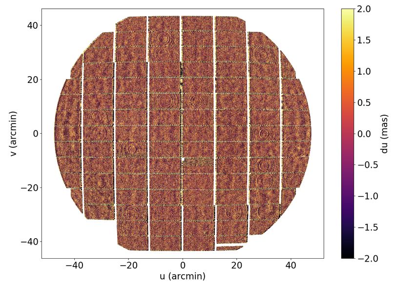
A&A proofs: manuscript no. main

of two back-to-back 15-s exposures: distortions induced by the             While we were finishing this paper, Fortino et al. 2020 (F20
                                                −1/2                   hereafter) produced a paper on the same subject using somewhat
atmosphere appear to scale empirically as T exp      (Heymans et al.
2012; Bernstein et al. 2017, B17 hereafter), where T exp is the in-    different techniques, and using the Dark Energy Survey (DES)
tegration time of an exposure. This turbulence contribution cor-       dataset. That work uses results from an astrometric solver de-
relates measured positions in an anisotropic fashion (as we will       scribed in B17, very similar to ours. The main differences be-
show later), with a spatial correlation pattern that varies from       tween the two works are due to the different sites (Cerro Tololo
exposure to exposure.                                                  vs. Mauna Kea), telescope sizes (4 m vs. 8 m), telescope mounts
                                                                       (equatorial vs. alt-az), and instruments (in particular, our instru-
     If shape measurements are performed on co-added images,
                                                                       ment is equipped with an atmospheric dispersion corrector). We
the astrometric residuals will affect the measured shapes of the
                                                                       will compare our results to F20 when relevant.
galaxies in a correlated way, and the point spread function (PSF)
of the co-added image in the same way. The challenge here is
to properly account for the complex correlation pattern for PSF        2. Astrometric solution and residuals from the
shape parameters, induced by the combination of anisotropic
                                                                          Hyper Suprime-Cam
components of varying orientation and correlation length. The
PSF of the co-added image has two components, one due to the           Hyper Suprime-Cam (HSC) is a prime-focus imaging instrument
actual PSF of the individual exposures, and one due to misreg-         installed on the 8.2-meter Subaru telescope. Its 104 2k×4k deep-
istration, in particular, due to turbulence-induced position shifts.   depleted CCD sensors cover about 1.7 deg2 on the sky. A de-
Since all input images do not contribute equally over the co-          tailed description of the instrument can be found in Miyazaki
added image area, it is common to transform all input images to        et al. (2018). The public data1 used in this study correspond to
the same PSF prior to co-adding, so that masked areas and gaps         observations acquired for the Deep and UltraDeep layers of the
between sensors do not cause PSF discontinuities on the sum.           Subaru Strategic Program2 (SSP). The data consist of a series of
This PSF homogenization does not cope with misregistration,            exposures of 180 s to 300 s, in each of the five optical bands of
which will then contribute small PSF discontinuities on the co-        the camera (grizy). In a given night, exposures in a given band
added image. In the framework of measurements performed on             are acquired in sequence, with a fixed orientation of the camera
individual exposures but relying on a common position estimate,        on the sky. The camera is equipped with an atmospheric dis-
one could perhaps devise a scheme to evaluate the shape correla-       persion corrector. The data analyzed in this paper correspond to
tions introduced by correlated position residuals, but this would      2294 exposures, imaged in two seasons of searches for transient
likely require a significant effort to attain the required accuracy.   objects using HSC (Yasuda et al. 2019): from November 2016
For the case of measuring light curves of distant supernovae, one      to May 2017 in the COSMOS field, and from March 2014 to
can readily evaluate the size of systematic position residuals for     November 2016 in the SXDS field.
a given exposure and correct the flux estimator for the induced
bias.
                                                                       2.1. Astrometric solution for HSC data
     If one aims to measure galaxy shapes on a large series of
short exposures, reducing the atmospheric contribution to astro-       We reduced the HSC data using classical procedures: simple
metric residuals will improve the usability of shape measure-          overscan and bias subtraction, implementation of a flat-field cor-
ments, mostly because of the complex correlation pattern of            rection from exposures acquired from an in-dome screen, detec-
astrometric shifts induced by the atmosphere. As we will dis-          tion of sources using SExtractor (Bertin & Arnouts 1996), com-
cuss later in this paper, reducing these astrometric residuals will    plemented by position estimations from a Gaussian profile fit to
be necessary for LSST cosmic shear measurements. Reducing              the detected sources, and an initial solution for the world coordi-
the astrometric systematics biases will also benefit other science     nate system (WCS) determined by matching the image catalogs
goals of Rubin Observatory – for example, trans-Neptunian ob-          to an external catalog (USNO-B), with typical residuals of 0.100 .
ject searches (see Bernardinelli et al. 2020 as an example), or the         We then performed a simultaneous astrometric fit to the cat-
measurement of proper motions of stars too faint to be measured        alogs for the images for each night and each band separately –
by Gaia (Ivezić et al. 2019).                                         5 to 15 images of the same field, with dithers of the order of
     In this paper, we investigate bulk trends of astrometric resid-   a few arc minutes. The WCS’s for the input images are used
uals presumably dominated by atmospheric turbulence, and aim           to associate the detections of the same astronomical sources in
to model these spatial correlations in order to reduce astromet-       different images. We simultaneously fit the geometrical transfor-
ric residuals. For this purpose we are using data from the Sub-        mations from pixel space to sky coordinates, and the coordinates
aru telescope equipped with the Hyper Suprime-Cam wide-field           of sources detected in at least two images. The fit is possible
camera. We first describe the Hyper Suprime-Cam, the data set,         because we constrain a small fraction of the detected source po-
and the reduction methods in Sec. 2, and justify the probable at-      sitions to their Gaia (Data Release 2, Gaia Collaboration et al.
mospheric origin of the observed position residuals (at least for      2018) positions on the date of observation; we call these sources
bright sources, where shot noise does not dominate). We then de-       the “anchors”. The geometric transformations are modeled as a
scribe in Sec. 3 the modeling of the spatial distribution of resid-    per-CCD mapping of pixel coordinates to an intermediate plane
uals as anisotropic Gaussian processes. In Sec. 4 we present our       coordinate, followed by a per-image mapping from this inter-
results, in particular the reduction in variances and covariances      mediate space to the tangent plane for this specific image. As
that the modeling provides. In Sec. 5, we average the a posteriori     such, this model is degenerate and we lift the degeneracy by im-
residuals in instrument coordinates in order to detect the small       posing that one of the per-image transformations is the identity
position distortions presumably due to sensors. In Sec. 6, we           1
                                                                          Public data can be found at https://hsc.mtk.nao.ac.jp/ssp/data-
evaluate the expected size of turbulence-induced position offsets      release/, and the raw images can be downloaded from
for Rubin Observatory, and estimate the spurious shear correla-        https://smoka.nao.ac.jp/HSCsearch.jsp
tions this causes if not corrected, under some reduction scheme         2
                                                                          Details of the SSP survey design and implementation can be found
We conclude in Sec. 7.                                                 at https://hsc.mtk.nao.ac.jp/ssp/ .

Article number, page 2 of 15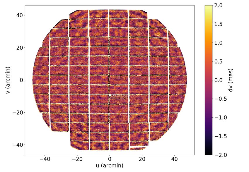
P.-F. Léget et al.: Astrometry & Gaussian processes

Fig. 1: Distribution of astrometric residuals in right ascension (du, left column) and declination (dv, center column), and displayed as vectors
(right column) for three individual exposures in z band, as a function of position in the focal plane, indexed in arcmin with respect to the optical
center of the camera. Gaps in the distributions are due to non-functionning CCD channels.

                                                                                                                      Article number, page 3 of 15
A&A proofs: manuscript no. main

transformation. The rationale for this two-transformation model                      70                   (exp id: 137108)
is that the per-CCD transformations capture the placement of the
                                                                                     60                                                 E-mode
CCDs in the focal plane and the optical distortions of the instru-                                                                      B-mode
ment, while the per-image transformations capture the variations                     50
from image to image due to both flexion of the optics and atmo-                      40

                                                                            (mas2)
spheric refraction3 . We initially model each transformation as                      30
a third-order polynomial – i.e., with 20 coefficients per trans-                     20

                                                                              E/B
formation, or ∼2000 parameters for the instrument geometry,
and 20 addtional parameters per image. The typical number of                         10
sources in a fit is ∼200,000, with a few thousands of these an-                       0
chored to Gaia. The least-squares minimization takes advantage                       10
of the sparse nature of the problem and runs in about 60 s for the                   20        100                      101
typical number of images (ten). The input uncertainties on the
measured positions account for shot noise only; therefore, we                                                   (arcmin)
add a position-error floor of 4 mas to all sources when comput-
                                                                            Fig. 2: Typical E- and B-mode correlation functions for a single 300-s
ing the weight used in the least-squares fit to avoid over-fitting          z-band exposure of HSC.
the bright sources.
     The analysis presented in the next section uses the residuals                   60
of this fit as input. The typical rms deviation of the astrometric                                                                 mean E-mode
residuals for HSC is between 6 and 8 mas for bright sources                          50                                            mean B-mode
(with the value depending on the band). The goal is to reduce                                                                      ±1 E-mode
the remaining dispersion and small scale correlations.                               40                                            ±1 B-mode

                                                                            (mas2)   30
2.2. Astrometric residuals of HSC
                                                                                     20
                                                                             E/B

We denote with du and dv the components of the astrometric
residual field within the local tangent plane, in right ascension                    10
and declination, respectively. In Fig. 1, we show examples of the
astrometric residuals, projected on the tangent plane, for three                      0
exposures. At this stage, the stochastic distortions affecting each
exposure are modeled, as described above, with a small num-                          10        100                      101
ber of parameters (typically 20). The spatial correlation of the                                               (arcmin)
residuals, and the variability of the correlation from exposure
to exposure, indicate that the parametrization with a third-order           Fig. 3: Average over all 2294 exposures of the E- and B-mode correla-
polynomial is not flexible enough to accommodate the observed               tion functions. The blue and red shaded area represent respectively the
variability. We see that the residuals exhibit a preferential direc-        standard deviation across nights of E- and B- mode.
tion that varies from exposure to exposure. This is very similar
to the residuals observed in DES and shown in B17.
     The spatial variations observed in the astrometric residuals           where dX(X) is the astrometric residual field on a complex form
exhibit preferential directions within an exposure; our hypothe-            (dX = du + idv) measured at a position X on the focal plane, r
sis, as in B17, is that these anistropies are mostly due to atmo-           is the distance between two positions, and β is the position angle
spheric turbulence. In this case (as discussed in B17), the astro-          of r. From ξ+ and ξ− we find the correlation functions ξE and ξB
metric residual field follows the gradient of the optical refractive        correponding to the E- and B-modes of the field:
index of the atmosphere in the telescope beam, averaged over                                         Z ∞
                                                                                   1         1            1
the integration time of the exposure. The two-point correlation             ξE = ξ+ (r) + ξ− (r) −          ξ− (r0 )dr0                    (3)
function ξ for the astrometric residual field has most generally                   2         2        r  r0
                                                                                                     Z ∞
two independent components, but only one if it is a gradient field                 1         1            1
and is curl free (Helmholtz’s theorem). The decomposition into a            ξB = ξ+ (r) − ξ− (r) +          ξ (r0 )dr0
                                                                                                           0 −
                                                                                                                                           (4)
                                                                                   2         2        r  r
curl-free E-mode and a divergence-free B-mode of vector fields
on the plane (B17) allows us to test the above hypothesis.                      We evaluate the correlation functions by calculating the co-
     Following B17 (see appendix A in particular), we evaluate              variance between the astrometric residuals for pairs of sources,
the two-point correlation functions ξ+ , ξ− , and ξ× for the astro-         in bins of spatial separation between the sources. From these, we
metric residual field,                                                      compute the binned version of E- and B-mode correlation func-
                                                                            tions. This involves an integral over separation (Eq. 37 in B17)
                                    h                i?                   that we evaluate by simply summing over each bin. With this
             ξ+ (r, β) = dX (X) e−iβ dX (X + r) e−iβ       ,     (1)
                                                                            binned estimation method, the integral of the correlation func-
                                                                            tions over angular separations is zero (see Appendix A).
                        D                           E
ξ− (r, β) + iξ× (r, β) = dX (X) e−iβ dX (X + r) e−iβ ,           (2)
                                                                                In Fig. 2, we show the correlation functions corresponding to
 3                                                                          the E- and B-modes for the single exposure shown in the bottom
   SCAMP (Bertin 2006) uses a similar parametrization for the same
problem. WCSFIT (B17) also implements a similar parametrization.            row of Fig. 1). Figure 3 shows the mean value calculated over the
Our software package, which was developed for Rubin Observatory,            2294 exposures of the Deep and UltraDeep layers of the SSP. We
takes advantage of sparse linear algebra techniques and solves for the      observe that the E-mode correlation function is non-zero while
sources’ positions, whereas B17 chose to treat source positions as latent   the B-mode correlation function is compatible with zero. This is
variables, which yields the same estimators.                                consistent with the result reported by DES in B17, for a different
Article number, page 4 of 15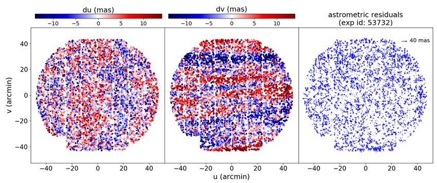
P.-F. Léget et al.: Astrometry & Gaussian processes

Fig. 4: Distribution of astrometric residuals in right ascension (du, left) and declination (dv, center), and displayed as vectors (right), as a function
of position in the focal plane. This z-band exposure corresponds to one of two nights when the focal plane was rotated through large angles during
the course of the night.

observing site and with a significantly different instrument. The             2.4. Nights with non zeros B-mode
HSC and DES results both indicate that the deplacement field
can be described as the gradient of a scalar field, which is likely           Another significant difference between the HSC results reported
the average over the line-of-sight of the optical refractive index            here and those of DES are that the astrometric residuals in ex-
of the atmosphere, as argued in B17. We also note that the mea-               posures for two HSC nights exhibit correlation functions with
sured correlation function has negative values at large separa-               B-mode contributions that are not negligible compared to the E-
tions; this is unavoidable, because the integral of the correlation           mode contributions, and E-mode values much larger than typi-
function is zero (see Appendix A). Moreover, the correlations                 cal. An example of the residuals for an exposure in such a night
that can be described by the fit of a third-order polynomial over             is shown in Fig. 4 and the corresponding correlation functions
the exposure data are much smaller than the observed correla-                 in Fig. 5. The Subaru telescope resides on an alt-azimuth mount;
tion, and should have a correlation length of about 0.4◦4 .                   the field derotator mechanism rotates only the focal plane, while
                                                                              the wide-field corrector remains fixed with respect to the tele-
                                                                              scope. Our astrometric model indexes the optical distortions of
2.3. Difference between HSC and DES results                                   the imaging system with respect to coordinates in CCD pixel
                                                                              space. Since in HSC, the image corrector rotates with respect
A notable difference between our results and those reported in                to the CCD mosaic, any breaking of the rotational symmetry of
B17 is the value of the correlation function as the angular sepa-             the optical distortions will cause spurious astrometric residuals.
ration approaches 0: Fig. 11 in B17, indicates a low-separation               As these residual only appear if exposures with different rotation
covariance of E-modes of the order of 80 milli-arcsec2 while we               angles are fit together, they tend to grow with the range of rota-
observe a value of 33 milli-arcsec2 for HSC; see Fig. 3. The fit-             tion angles involved in the fit. These residuals are not induced
ting algorithms used to calculate the residuals are similar. How-             by the gradient of a scalar field, and hence are prone to similar
ever, there are two important quantitative differences: the expo-             amounts of E- and B-modes. The nights with large B-mode con-
sure times are longer for HSC (∼270 s vs. 90 s for DES), and                  tributions are characterized by a large rotation of the focal plane
the mirror diameter of the Subaru telescope is about twice as                 over the course of the observations, mostly because the observa-
large as that of the Blanco Telescope (where DES observed). The               tions were spread over several hours, and sometimes most of the
variance attributed to atmospheric effects typically scales as the            night. Our astrometric model does not compensate for this rota-
inverse of the exposure time (Heymans et al. 2012), while the                 tion (and neither does the one in B17), both because we were not
dependence on aperture is more complicated, but favors larger                 aware of the details of the HSC mechanics before discovering
apertures. Finally, the Subaru telescope is located at an elevation           these large rotations, and because the astrometry software we are
of 4400 m at the summit of Mauna Kea in Hawaii, while the                     using was originally developed for reducing the Canada-France-
Blanco telescope is at an elevation of only 2200 m at the Cerro               Hawaii Telescope (CFHT) Legacy Survey, and the CFHT has
Tololo Inter-American Observatory (CTIO) in Chile.                            an equatorial mount. The fitted model would have to be heavily
                                                                              modified to account for these rotations, as noted in B17, for only
                                                                              the two night impacted by these large rotations. Most of our fits
                                                                              include images acquired over less than an hour and the whole
4
   Since the size of the field of view is 1.7 deg2 , and 10 parameters        rotation range is typically less than 20◦ .
per component are fit for the third-order polynomial, each parameter
describes an area of ∼0.17 deg2 , which corresponds to an angular scale           Other than these two nights with large focal plane rotations,
of ∼0.4◦                                                                      the astrometric residuals exhibit a covariance pattern that can be
                                                                                                                          Article number, page 5 of 15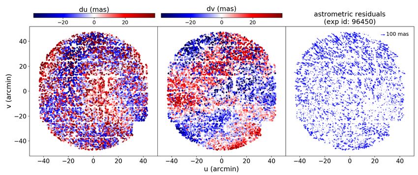
A&A proofs: manuscript no. main

         300                   (exp id: 96450)                             y0 ≡ E[y], where E[x] denotes the expectation value of the ran-
                                                             E-mode        dom variable x. Because the field is Gaussian (i.e., y is Gaussian
         250                                                 B-mode        distributed at any position X), the distribution is Gaussian:

         200                                                               y ∼ N(y0 , ξ(0)),                                                         (5)
(mas2)

         150                                                               where ξ is the correlation function:
 E/B

         100                                                               ξ(X 0 − X) ≡ Cov(y(X), y(X 0 )).                                          (6)
         50                                                                    In the context of modeling astrometric residuals, y can be ei-
                                                                           ther of the components du or dv, and X is the coordinate in the
          0                                                                local tangent plane. GP interpolation is a method for estimating
                    100                      101
                                    (arcmin)                               the value of the field at arbitrary locations, given a realization of
                                                                           the field at a set of (usually different) locations. In practice, the
Fig. 5: Typical E- and B-mode correlation function for the same expo-      kernel ξ is unknown – or at least its parameters are unknown.
sure shown in Fig. 4, corresponding to one of two nights when the focal    We will discuss their determination in the next section. The co-
plane was rotated through large angles.                                    variance matrix for the data realization is calculated and used in
                                                                           the interpolation. The covariance matrix will be positive definite
                                                                           (which is required for it to be invertible in a later step) for any set
mostly attributed to atmospheric turbulence. In the next section,          of locations if and only if the correlation function ξ has a posi-
we describe how we model these residuals.                                  tive Fourier transform (Bochner’s Theorem). This constrains the
                                                                           shape of possible correlation functions.
3. Modeling astrometric residuals using anisotropic                            We now describe the practical interpolation method. We have
                                                                           a realization yi at positions Xi , and we assume for now that we
   Gaussian processes                                                      know the kernel ξ. The covariance matrix C of the y realization
Spatial variations in the refractive index of the atmosphere can           is given by:
be described as a Gaussian random field, which must be station-
ary (that is, the covariance between values at different points de-        Ci j ≡ Cov[yi − y0 (Xi )), y j − y0 (X j )] = ξ(X j − Xi ) + δi j σ2i ,   (7)
pends only on their separation) because there is no special point
                                                                           where σi is the measurement uncertainty of yi .
in the image plane. We therefore model the astrometric resid-
                                                                               The expectation of the Gaussian field at locations y0 , given
ual field in the image plane as a Gaussian process (GP), which
                                                                           the values of y at locations X0 , is (Rasmussen & Williams 2006):
allows us to correct for astrometric residuals in the data, account-
ing for the correlations introduced by the Gaussian random field.
In Sec. 3.1, we briefly introduce GPs, describe how the astromet-          y0 = Ξ(X0 , y)C−1 (y − y0 ) + y0 ,                                        (8)
ric residual field can be modeled as a GP, and discuss possible
strategies for optimization of the GP. In Sec. 3.2, we describe the        where Ξ is a matrix with elements defined by
method we use for the optimization of the GP hyperparameters,
and our choice for the analytical correlation function. This GP            Ξ( A, B)i j ≡ ξ( Ai − B j ).                                              (9)
interpolation was originaly developped for interpolating the at-
mospheric part of the PSF in the context of DES (Jarvis et al.             The covariance of the interpolated values is:
2021) and follow a similar scheme of interpolation.                         h                               i
                                                                           E (y0 − y0 (X0 ))(y0 − y0 (X0 ))T =
3.1. Introduction to Gaussian processes                                                              Ξ(X0 , X0 ) − Ξ(X0 , X)T C−1 Ξ(X0 , X). (10)
In this subsection, we give a brief overview of classical GP inter-
                                                                               We see from Eq. 8 that, in the absence of measurement un-
polation5 ; a more detailed description can be found, for example,
                                                                           certainties σi , the interpolated values at the training points X are
in Rasmussen & Williams (2006). A GP is the optimal method
                                                                           just the y values with no uncertainties. This is because the inter-
for interpolating a Gaussian random field. GP interpolation can
                                                                           polation method delivers the average expected field values given
be used for irregularly spaced datasets and, because it operates
                                                                           y(X) with covariance C. In practice, the matrix C (defined in
by describing the correlations between data rather than follow-
                                                                           Eq. 7) is numerically singular or almost singular if there are no
ing a specific functional form6 , is very flexible. In practice, one
                                                                           measurement uncertainties σi , even for sample sizes as small as
must choose both the analytic form of this correlation function
                                                                           20; in the case of zero uncertainty, a small noise value should be
(also called a "kernel") and the parameters for this kernel (often
                                                                           added for the above expressions to be numerically stable.
called "hyperparameters") that describe the second-order statis-
                                                                               The interpolation method is now well-defined, given a data
tics of the data.
                                                                           realization and a choice of kernel. A commonly used kernel is
    A stationary Gaussian random field is entirely defined by its
                                                                           the Gaussian kernel (also known as a squared exponential),
mean value (as a function of position) and its second-order statis-
tics, which depend only on separation in position. We denote                                      "
                                                                                                     1
                                                                                                                                   #
the (scalar) Gaussian random field as y and its mean value as              ξ (X1 , X2 ) = φ exp − (X1 − X2 ) L (X1 − X2 ) ,
                                                                                            2                    T −1
                                                                                                                                            (11)
                                                                                                     2
5
   Also referred to as ordinary kriging or as Wiener filtering.
6
   This feature of GPs results in the descriptor "non-parametric," which   where X1 and X2 correspond to two positions (in the focal plane
simply means GPs are not from a parametric family of distributions. As     for our case), φ2 is the variance of the Gaussian random field
with any interpolation method, a GP requires setting parameter values.     about the mean function y0 (X), and the covariance matrix L is in
Article number, page 6 of 15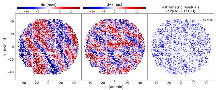
P.-F. Léget et al.: Astrometry & Gaussian processes

general anisotropic since atmospheric turbulence typically has a                                        104
                                                                                                                    Maximum Likelihood

                                                                         Computational time (seconds)
preferred direction due to wind direction:
                                                                                                                    2-point correlation function
                                                                                                        103
                   !T 2
       cos α sin α    `                cos α sin α
                                     !              !
                                 0
L=                                                    ,          (12)
      − sin α cos α   0        (q `)2 − sin α cos α

where α represents the direction of the anisotropy, ` represents                                        102
the correlation length in the isotropic case, q is the ratio of the
semi-major to semi-minor axes of the ellipse associated with the
covariance matrix7 .                                                                                    101
    Although a Gaussian kernel is often used, we can choose
an analytical form for the kernel based on empirical consider-
ations and/or the relevant physics. Both the functional form of                                         100
the kernel and the hyperparameters associated with the kernel                                                     103                                        104
determine the interpolated estimates. Once the kernel shape is                                                                       # of points
chosen, the parameters can be determined with a maximum like-
lihood fit, where the likelihood of the realization y (of size N) is           Fig. 6: Typical computational time necessary to determine hyperpa-
defined by                                                                     rameters as a function of the number of data points used during training
                                                                               for a classical maximum likelihood method using Cholesky decompo-
                                                                               sition (red triangles) and when using the two-point correlation function
                                                             !
        1          1              1
L= √ N × √               × exp − y − y0 T C−1 y − y0 . (13)

                                                                               computed by TreeCorr (blue circles). The typical number of training
       2π        det(C)           2                                            points for astrometric residuals modeled using GPs is between ∼ 103
                                                                               and ∼ 104 .
    Maximizing this expression with respect to the parameters of
ξ that define C (via Eq. 7) is numerically cumbersome because it
involves many inversions (in practice, factorizations) of the co-              size (see section 4.1 of Jarvis et al. 2004), and it proves partic-
variance matrix C, which has the size of the “training sample”                 ularly efficient for data sets of a size relevant to PSF interpola-
y. The factorisation (for example, the Cholesky decomposition)                 tion, where it scales roughly linearly with the number of input
also trivially delivers the needed determinant. The time to com-               data points. Figure 6 shows the computational time for the max-
                                                                               imum likelihood approach and the estimation of hyperparam-

                                           3
pute such a factorisation scales as O N , where N is the size
of the training sample y. It is possible to speed up the inver-                eters based on the binned two-point correlation function using
sion of the matrix C in Eq. 13 under certain assumptions. For                  TreeCorr, as a function of the number of data points; the latter
example, Ambikasaran et al. 2015                                             technique is several orders of magnitude faster for the training
                                   propose to speed-up the ma-               sample sizes we are contemplating (between ∼ 103 and ∼ 104 ).
trix inversion from O N 3 to O N log2 (N) based on a special                       We estimate the covariance matrix of the binned two-point
decomposition of the matrix (HODLR). Other methods achieve                     correlation function via a bootstrap (done on sources). This mea-
O (N) under certain assumptions about the analytical form of the               sured covariance matrix is then used in the fit of the analytical
kernel and by being limited to one dimension (Foreman-Mackey                   model for the kernel to the measured two-point correlation func-
et al. 2017).                                                                  tion in a non-diagonal least-squares minimization. These three
    Here, we follow another route, which relies on the good                    steps (binned two-point correlation function, bootstrap covari-
sampling provided by the training sample. From the smooth-                     ance matrix, least-squares fit) are included in the computational
ness of the measured correlation function in Fig. 2, we can con-               times shown in Fig. 6.
clude that the average distance to the nearest neighbors is much                   Although the Gaussian kernel is often used for GP interpo-
smaller than the correlation length. Therefore, we can estimate                lation, for ground-based imaging, a kernel profile with broader
the anisotropic correlation function directly from the data. The               wings is expected to provide a better description of the longer-
practical implementation is described in the next section.                     range correlations present in PSF dominated by atmospheric tur-
                                                                               bulence (see, for example, Fig. 2 in Roddier 1981). To account
3.2. Hyperparameter estimation using the two-point                             for the clear anisotropy in the correlation function, we use an
     correlation function                                                      anisotropic von Kármán kernel as proposed in Heymans et al.
                                                                               2012 to describe the observed spatial correlations of PSF distor-
Estimating the kernel of a stationary GP directly from the two-                tions for CFHT and is parametrised as
point statistics was pioneered in the field of geostatistics (see
Cressie 1992 for example). The time to compute     the two-point                                     T
                                                                                                                      65
                                                                             ξ Xi , X j = φ × Xi − X j L Xi − X j ×
                                                                                                           −1       2
correlation function naively scales as O N 2 ; however, faster

approaches have been developed. We use a package called                                                            T
                                                                                                  K−5/6 2π Xi − X j L−1 Xi − X j , (14)
TreeCorr (Jarvis et al. 2004), which evaluates covariances in
distance bins for large datasets. Our implementation of the es-
                                                                               where the notation is the same as for Eq. 11 and K is the mod-
timation of hyperparameters using TreeCorr can be found on-
                                                                               ified Bessel function of the second kind. At large separations, ξ
line8 . The computational time for TreeCorr depends on the bin
                                                                               decays exponentially. We show in Fig. 7 Gaussian and von Kár-
 7
   Can be written as a function of the image distortion parameters g1          mán kernels of similar widths. As we will soon show, a von Kár-
and g2 . This parametrization of the covariance matrix is analogous to         mán kernel reduces the residuals more efficiently than a Gaus-
that used in cosmic shear; see, for example, equation 7 in Schneider           sian kernel.
et al. 2006.                                                                       One may wonder why we rely on a parametrized form of the
 8
   https://github.com/PFLeget/treegp                                           kernel, typically with a small number of parameters (four here),
                                                                                                                                               Article number, page 7 of 15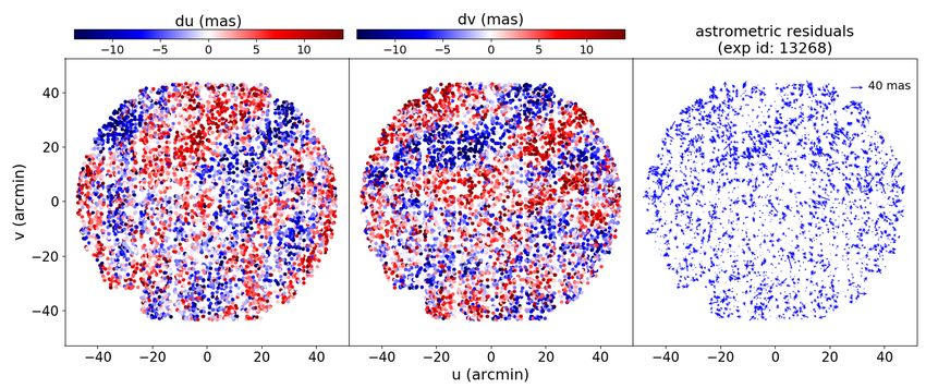
A&A proofs: manuscript no. main

      1.0                                                Gaussian           GP fit. We fit the two projections of the residuals as independent
                                                         von Kármán         GPs, and ignore cross correlations.
                                                                                As discussed earlier, GPs simply reproduce the input data
      0.8                                                                   if interpolation at an input data point is requested, at least in
                                                                            the absence of measurement noise. Therefore, in order to use
      0.6
(r)

                                                                            residuals to evaluate the GP performance in an unbiased way,
                                                                            we randomly select a “validation sample” consisting of 20% of
      0.4                                                                   the sources fully qualified for training, that we exclude from the
                                                                            training sample. We then compute the GP interpolation for all
      0.2                                                                   sources used in the astrometry (i.e., all sources with an aperture
                                                                            flux delivering a signal-to-noise ratio greater than 10). The per-
      0.0                                                                   formance tests described in this section (unless otherwise speci-
            0      1           2        3         4         5          6    fied) are computed only on this validation sample.
                                        r                                       The result of the GP modeling of the astrometric residual
                                                                            field for a single exposure in z-band is shown in Fig. 8 (see cap-
Fig. 7: Gaussian kernel compared to the von Kármán kernel that is
used in this analysis. The width of the latter was determined by a least-   tion for detail). The measured correlation functions have nega-
squares fit to the former.                                                  tive lobes because they integrate to zero. The positive analytical
                                                                            function cannot obviously reproduce those negative parts. We
                                                                            add a constant floor k in order to allow the kernel to have neg-
rather than using a more empirical fit (for example with spline             ative lobes and to not bias hyperparameters estimation. Conse-
functions) of the measured correlation function. As discussed               quently, the following equation is minimized in order to find the
earlier, a correlation function should have a positive Fourier              best set of hyperparameters θ:
transform and, if it does not, the covariance matrix of obser-
vations (Eq. 7 for σi = 0) is not positive-definite for all real-                            T
izations. Therefore, when smoothing the measured correlation                χ2 = ξ − ξ̂(θ) − k W ξ − ξ̂(θ) − k ,                                 (15)
function, one should restrict the outcome to functions with posi-
tive Fourier transforms. Splines cannot in general be guaranteed            where ξ is the measured two-point correlation function, ξ̂ is the
to have positive Fourier transforms. Both Gaussian and von Kár-             analytical kernel (gaussian or von Kármán), W is the inverse
mán kernels fulfill this requirement, so we only consider these             of the covariance matrix of the measured two-point correlation
two models. We note that a maximum likelihood approach faces                function, and k which is the constant not taken into account when
the same constraint of having a correlation function with a posi-           computing the final kernel and consequently when computing
tive Fourier transforms.                                                    the GP interpolation (Eq. 8). The von Kármán kernel fits well
                                                                            the principal direction of the anisotropy and delivers a reason-
                                                                            able correlation length. However, one can see that by looking at
3.3. Difference with DES GP modeling                                        the two-point correlation function residuals on the third row of
We now describe the main differences with the approach cho-                 Fig. 8 that the von Kármán profile does not fit perfectly the ob-
sen in F20. First, we do not enforce the model to describe a                served kernel, even if it does a better job than the classic Gaus-
gradient field; rather we model and fit independently the two               sian kernel (see below). A room for improvement would be to
spatial components. In F20, the authors eventually optimize the             have a more flexible kernel to describe the observed two-point
kernel hyperparameters in order to minimize the average covari-             correlation, such as a spline basis9 , but lies beyond the scope of
ance on small angular scales, while we simply fit the hyperpa-              this analysis.
rameters to the empirical covariance. We speculate whether this                 We show in Fig. 9 the correlation functions for the E- and
optimization is necessary and whether it will be viable when it             B-modes of the astrometric residual field calculated for the vali-
comes to large scale production as required by the processing of            dation sample in a representative exposure (same as the one pre-
Rubin Observatory data. Second, the anisotropy of the correla-              sented in Fig. 8), before and after GP modeling and interpolation
tions in F20 is entirely attributed to the wind-driven motion of a          with a von Kármán kernel. We see a significant reduction in E-
static phase screen during the exposure, and we have not tested             mode correlation function after GP interpolation.
whether this assumption improves our results. Third, We model                   We show in Fig. 10 the E and B-mode correlation functions
the correlation function with four parameters, while F20 use five,          calculated for the validation sample and averaged over all 2294
where the fifth parameter is the outer scale and we expect its in-          exposures, before (top plot) and after GP interpolation with a
fluence on the correlation function to be small. Finaly, we have            Gaussian kernel (center plot) and a von Kármán kernel (bottom
not rejected outliers in the GP fit; i.e., sources exhibiting large         plot), together with the ±1-σ spread over exposures. GP inter-
a posteriori residuals are not removed from the training sample,            polation reduces the magnitude of the correlation function by
but a priori outliers have been removed.                                    almost one order of magnitude, from 30 mas2 to 3 mas2 at small
                                                                            scales. The von Kármán kernel performs better than the Gaus-
                                                                            sian kernel. We can also see the improvement by comparing the
4. Correcting astrometric residuals using                                   dispersion of the astrometric residuals with the flux as in Fig. 11.
   anisotropic Gaussian processes                                           9
                                                                               We tried to fit the observed two-point correlation function using a
                                                                            spline basis, but it did not produce a positive definite covariance matrix
We apply GP interpolation to the astrometric residuals for the              of the residuals. A solution might be to fit a spline basis on the Fourier
2294 exposures of the SSP in the five bands. We train the GP on             transform of the observed two-point correlation function instead and
the unsaturated sources with magnitudes brighter than 20.5 AB               ensure that the fit is positive in Fourier space. This procedure should
mag. The residuals are clipped at 5-σ during the prior astromet-            produce a positive definite covariance matrix of residuals (Bochner’s
ric fitting process but, in contrast with F20, we do not clip in the        Theorem).

Article number, page 8 of 15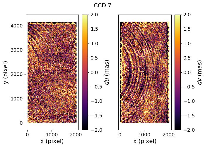
P.-F. Léget et al.: Astrometry & Gaussian processes

Fig. 8: GP fit of astrometric residuals for a single 300-s z-band exposure. The fit is done independently for each component of the vector field. The
top six plots show results for the du component, and the bottom six plots for the dv component. The plots in the top row within each group illustrate
how the hyperparameters are determined from a von Kármán kernel (center plot) fit to the measured two-point correlation function calculated for
80% of the training sample (left plot); the difference between the measured two-point correlation function and the best-fit von Kármán kernel is
shown in the right-most plots. The plots in the bottom row within each group of six represent the variation across the focal plane of the measured
component of the astrometric residual field, the astrometric residual field predicted by the GP using the best-fit hyperparameters, and the difference
between measure and fit, projected in the local tangent plane for the 20% of sources in the validation sample.

                                                                                                                        Article number, page 9 of 15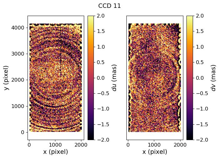
A&A proofs: manuscript no. main

                                exp: 137108                                                                 No correction
                                                                                    60       E(0) = (29 ± 29) mas2 | B(0) = (1 ± 20) mas2
         60
                                                                                                                                mean E-mode (test)
                                                                                    50                                          mean B-mode (test)
         40                                                                                                                     ±1 E-mode
                                                                                    40                                          ±1 B-mode
(mas2)

                                                                           (mas2)
         20                                                                         30
                                                                                    20
 E/B

                                                                            E/B
          0
                                                                                    10
                                            E-mode (no GP correction)
         20                                 E-mode (GP corrected)                    0
                                            B-mode (no GP correction)
                                            B-mode (GP corrected)                   10
         40         100                     101
                                                                                               100                       101
                                                                                                               (arcmin)
                                    (arcmin)
                                                                                                 GP corrected with Gaussian kernel
Fig. 9: Correlation functions corresponding to E- (blue) and B- (red)               60       E(0) = (6 ± 13) mas2 | B(0) = (1 ± 13) mas2
modes of the astrometric residual field on the validation sample for a                                                  mean E-mode (test, after GP)
representative exposure (one of three exposure shown in Fig. 1), before             50                                  mean B-mode (test, after GP)
applying the GP interpolation correction (circles) and after correction                                                 ±1 E-mode
(crosses)                                                                           40                                  ±1 B-mode

                                                                           (mas2)
                                                                                    30
As for the E-mode reduction, it can be seen that after correcting
                                                                                    20
                                                                            E/B
by the GP interpolation, GP reduces the dispersion by a factor of
two and the von Kármán kernel does a better job than the classi-                    10
cal Gaussian kernel by ∼ 20% in rms.
     We investigated whether the a posteriori residuals are sen-                     0
sitive to the size of the training set, and found no compelling
differences between results for exposures with 2000 and 6000                        10         100                       101
training sources. We interpret this as an indication that the mod-                                             (arcmin)
eling is not limited by the image plane sampling or the shot noise                             GP corrected with von Kármán kernel
affecting position measurements, but rather by the ability of the
                                                                                    60       E(0) = (3 ± 12) mas2 | B(0) = (1 ± 12) mas2
kernel to describe the correlation. Therefore, reducing the num-                                                        mean E-mode (test, after GP)
ber of training points is an immediate avenue to reducing com-                      50                                  mean B-mode (test, after GP)
putational demands, and further work should focus on modeling                                                           ±1 E-mode
of the kernel.                                                                      40                                  ±1 B-mode
                                                                           (mas2)

                                                                                    30
5. Average residuals in CCD coordinates                                             20
                                                                            E/B

Sensor effects that are not modeled with the GP (e.g., fabrica-                     10
tion defects in the CCD, or distortions in the drift fields) can
appear in an image of the average residuals over the focal plane.                    0
In Fig. 12, we show the average value over all the exposures
of the two components of the residuals for three representative                     10         100                       101
CCDs. One can see two main types of defects: so-called "tree                                                    (arcmin)
rings", and "scallop-shaped" structures near the edges of the sen-
sors. The former are commonly attributed to the variation in the          Fig. 10: Average over all 2294 exposures of the E- and B-mode corre-
density of impurities, with a symmetry due to how the crystals            lation functions, calculated on the validation sample, for different mod-
are grown. The latter are likely due to mechanical stresses ap-           eling choices. Top: Correction from GP interpolation is not applied.
plied to the silicon lattice, induced by the binding of the sensor        Middle: correction from GP interpolation is applied using a Gaussian
to its support structure. The DECam sensors exhibit similar de-           kernel. Bottom: correction from GP interpolation is applied using a von
fects, as shown in B17, but at about an order of magnitude larger         Kármán kernel. For all those plots, the blue and red shaded area rep-
                                                                          resent respectively the standard deviation across nights of E- and B-
scale. The sizes of the tree-ring residuals are ∼ 2 mas for HSC           mode.
and ∼ 13-26 mas for DECam (Plazas et al. 2014). We have not
been able to find in the literature previous mention of these tiny
defects on HSC sensors. The rms astronomical residuals associ-
ated with the scallop-shaped features in the images for the HSC           band will differ only on a global scale due to the variation with
CCDs are ∼10 mas – larger than those associated with the tree-            wavelength of the average conversion depth of photons in sili-
ring features.                                                            con. We mildly confirm that redder bands have weaker patterns,
     In order to clearly see these small effects (mostly below 10         as expected, but we could not devise a robust measurement of ra-
mas), we averaged all bands together since the signal in indi-            tios between bands. Averaging in larger spatial bins smears the
vidual bands is very noisy. We expect that the patterns in each           smaller structures. If we apply these patterns as a mean function
Article number, page 10 of 15
P.-F. Léget et al.: Astrometry & Gaussian processes
16
du dv
14
12 No GP correction
GP corrected | Gaussian kernel
10 GP corrected | von Kármán kernel
wRMS (mas)
GP corrected | von Kármán kernel
8 + mean function
6
4
2
0
23 22 21 20 19 18 23 22 21 20 19 18
Apparent AB mag Apparent AB mag
Fig. 11: Weighted RMS of astrometric residuals as a function of apparent AB magnitude of the source for each component of the astrometric
residual field. Four models are compared: no correction from a GP interpolation (red circles), correction from a GP interpolation with a Gaussian
kernel (black crosses), correction from a GP interpolation with a von Kármán kernel (blue stars), and correction from a GP interpolation with a
von Kármán kernel and the mean function computed as described in Sec. 5 (green triangles, hidden underneath the blue ones).
of the GP, the improvement of the residuals (both in variance and purely due to these turbulence-induced residuals, for 30-s expo-
covariance) is below 1 mas2 (cf. Fig. 11). However, recomputing sures in the Rubin Observatory, assuming they are not mitigated.
the mean function and taking it into account in the GP modeling Measuring shear without co-adding images requires measur-
allows us to remove most of the patterns observed in individuals ing second moments using galaxy positions averaged over im-
CCDs as shown in Fig. 13. ages, because the position noise biases the second moments (this
The HSC instrument is characterized by a rapid evolution is the so-called noise bias). Using average positions is partic-
of the plate scale in the outer part of the focal plane: the linear ularly required for the Rubin observatory where the final image
plate scale varies by 10% between the center and the edge of depth is obtained from hundreds of short exposures in each band.
the field, and 70% of this variation is concentrated in the outer In order to evaluate the effect of displaced positions on cosmic
30% radius. In order to verify that our modeling can cope with shear signal, we shift positions coherently on small spatial scales
this variation, we plot the residuals in the whole focal plane, in by dx in a single exposure. Using a Taylor expansion, we derive
order to check for systematic residuals at the few mas level in the shear offset in the astrometric residual direction to be
Fig. 14. The model consists of one polynomial transformation !2
per sensor from pixel coordinates to the tangent plane, common 1 dx
δγ ' , (16)
to all exposures. We see in Fig. 14 that there are residuals when 4 σg
using third-order polynomials per CCD, which disappear with
fifth-order polynomials. However, all the astrometric residuals independent of the size of the PSF, where δγ is the shear bias
used in the GP modeling used the third-order polynomials per and σg denotes the r.m.s. angular size of the galaxy, and dx the
CCD. (spurious) position shift. The general expression, accounting for
actual directions, reads
!2
6. Impact of correlations in astrometric residuals on 1 dx + i dy
δγ1 + iδγ2 ' . (17)
cosmic shear measurements 4 σg
We explained above that Rubin Observatory will need to model where γ1 describes shear along the x or y axes, and γ2 the shear
the astrometric distortions from the atmosphere because of the along axes rotated by 45◦ , as defined in Schneider et al. (2006).
short exposures (two back-to-back 15-s exposures) defined in Therefore, the shear covariances induced by covariances of posi-
the current observing plan. We measure for HSC a small-scale tion offsets involve the covariance of squares of position offsets.
covariance in astrometric residuals of about 30 mas2 for an av- For centered Gaussian-distributed variables X and Y, we have
erage exposure duration of 270 s. The Rubin Observatory tele-
scope has a smaller effective primary mirror area than the Sub- Cov(X 2 , Y 2 ) = 2 [Cov(X, Y)]2 , (18)
aru telescope and is located at a lower elevation, so we expect
atmospheric effects to be more significant at Rubin Observatory. which allows us to relate the correlation function of shear to the
Neglecting these differences, and assuming that covariances vary correlation function of position offsets. In order to evaluate the
only as the inverse of the exposure time, we would expect 540 impact of spatially correlated position offsets on measured shear
mas2 and 270 mas2 of small-scale covariance on average for Ru- spatial correlations, we consider the smallest galaxy sizes used in
bin Observatory exposures of 15 s and 30 s, respectively. These DES Y1 (Zuntz et al. 2018), which have σg ' 0.200 . Their shear
covariances affect in a coherent way the astrometric residuals, will experience an additive offset of ∼ 1.6 × 10⁻³ (for a small
and can extend up to 1 degree, along the major axis of the corre- scale correlation of 270 mas2 ), which will bias the shear correla-
lation function. Those may affect the measurement of shear, and tion function by ∼ 6 × 10⁻⁶ , which is about half of the expected
we will now provide a rough estimate of the shear correlation cosmic shear signal at z ∼ 0.5 and 10 arcmin separation.
Article number, page 11 of 15A&A proofs: manuscript no. main
Troxel et al. 2018. The regions shaded in red in Fig. 15 in each
tomographic bin represent the angular scales that were removed
in the Troxel et al. 2018 analysis because they could be signifi-
cantly biased by baryonic effects. The blue area in Fig. 15 in each
of the tomographic bins represent the contribution to the cosmic
shear signal due to the average spatial correlations of the astro-
metric residuals due to atmospheric turbulence scaled from the
HSC average measurement to 30-s exposures. This adds to shear
a contribution comparable to the DES Y1 uncertainty, which is
considerably larger than the LSST precision goal. These corre-
lated position offsets were not an issue for previous surveys like
DES because the variance of the astrometric residuals in DES
is 3 times lower than that expected for LSST, and therefore the
contribution to the shear correlation function is 10 times lower
since is scales as the square of the variance. It is unlikely that
the wind direction projected on the sky would average out this
effect, because the wind direction at an observatory has a pre-
ferred direction, on average. If we are able to reduce the position
covariances down to a few mas2 , the effect on the shear correla-
tion functions becomes 2 to 3 orders of magnitude smaller than
the cosmic shear signal itself.
We have described a measurement scheme where galaxy po-
sitions are affected by turbulence-induced offsets. If one per-
forms an image co-addition prior to shear measurement, the co-
addition PSF will account for the position offsets, and hence the
shear measurements may be free of the offsets described above.
This is true for regions covered by all exposures, but there are
discontinuities of both PSF and the atmospheric-induced shear
field where the number of exposures involved in the co-addition
changes. Note also that the atmospheric-induced offsets cause a
PSF correlation pattern that may prove difficult to discribe accu-
rately. Therefore, for short exposure times, even if one co-adds
images and then measures shear, one probably has to accurately
model the spatial correlations in the atmospheric-induced posi-
tion shifts down to arc-minute scales.
7. Conclusions
We have studied astrometric residuals for bright stars measured
in exposures acquired with the HSC instrument on the Subaru
Fig. 12: Average of the astrometric residual field for each component telescope, and find that these residuals are dominated by E-
projected in pixel coordinate for 3 different chips with some character- modes. We have developed a fast GP interpolation method to
istic features that can be also found on the other chips. model the astrometric residual field induced by atmospheric tur-
bulence. We find that a von Kármán kernel performs better than
a Gaussian kernel, and the modeling reduces the covariances of
In Fig. 15, we display both the expected cosmic shear sig- neighboring sources by about one order of magnitude, from 30
nal and the contribution from the position offsets derived from mas2 to 3 mas2 in variance, and the variances of bright sources
the average HSC measurement, scaled to 30-s exposures, as- by about a factor of 2. Those reductions using GP interpolation
suming those offsets are not mitigated. This prediction assumes are really similar to recent result published in F20 with the DES
that the shear is measured on individual exposures, using a com- dataset. Based on simulations of atmospheric distortions above
mon average position with no GP modeling and correction of at- the Rubin Observatory telescope, we find that, for short expo-
mospheric displacements. The cosmic shear signal in Fig. 15 is sures, the correlated astrometric residuals may cause a spurious
computed in the four tomographic bins used in the cosmic shear contribution to shear correlations as large as the cosmic signal.
analysis of Troxel et al. 2018; the shear correlation functions ξ+ Mitigating these turbulence-induced offsets, possibly along the
are computed using the Core Cosmology Library (Chisari et al. lines we have sketched in this paper, will be necessary for cos-
2019) with the fiducial cosmology result from Troxel et al. 2018 mic shear analyses. We have shown that the spatial correlation
(black curve in Fig. 15). The comic shear signal presented in of astrometric residuals can be significantly lowered by model-
Fig. 15 takes into account the non-linearity of the matter power ing and then correcting these residuals using GP interpolation.
spectrum and the spatial correlations introduced by the intrinsic We find that it is necessary to incorporate this modeling in the
alignment as in Troxel et al. 2018. For a representation of the cur- astrometric fit itself (as opposed to the GP interpolation done in
rent knowledge of the cosmic shear signal, we indicate in Fig. 15 post-processing and described in Sec. 3 and Sec. 4) in order to
with a dark region around the cosmic shear correlation function achieve more precise and accurate average source positions and
the variations on S 8 (σ8 (Ωm /0.3)0.5 ) of ±0.027, which represent pixel-to-sky transformations. The post-processing can be done
the ±1σ uncertainty from the fiducial cosmic shear analysis of along the lines sketched in the presented analysis, namely find-
Article number, page 12 of 15You can also read