IO Workload Characterization Revisited: A Data-Mining Approach
←
→
Page content transcription
If your browser does not render page correctly, please read the page content below
3026                                                                                        IEEE TRANSACTIONS ON COMPUTERS, VOL. 63, NO. 12, DECEMBER 2014

              IO Workload Characterization Revisited:
                     A Data-Mining Approach
                                  Bumjoon Seo, Sooyong Kang, Jongmoo Choi, Jaehyuk Cha,
                                    Youjip Won, and Sungroh Yoon, Senior Member, IEEE

       Abstract—Over the past few decades, IO workload characterization has been a critical issue for operating system and storage
       community. Even so, the issue still deserves investigation because of the continued introduction of novel storage devices such as
       solid-state drives (SSDs), which have different characteristics from traditional hard disks. We propose novel IO workload characterization
       and classification schemes, aiming at addressing three major issues: (i) deciding right mining algorithms for IO traffic analysis,
       (ii) determining a feature set to properly characterize IO workloads, and (iii) defining essential IO traffic classes state-of-the-art storage
       devices can exploit in their internal management. The proposed characterization scheme extracts basic attributes that can effectively
       represent the characteristics of IO workloads and, based on the attributes, finds representative access patterns in general workloads
       using various clustering algorithms. The proposed classification scheme finds a small number of representative patterns of a given
       workload that can be exploited for optimization either in the storage stack of the operating system or inside the storage device.

       Index Terms—IO workload characterization, storage and operating systems, SSD, clustering, classification

1      INTRODUCTION
         of 2013, NAND flash prices are finally below one US
A      S
      dollar per gigabyte [1], [2], and NAND-based SSDs are
quickly gaining momentum as the primary storage device in
                                                                                           IO workloads. However, existing characterization efforts for
                                                                                           HDDs and virtual memory fail to meet the characterization
                                                                                           requirements for NAND-based storage devices. Over the past
mobile platforms, notebooks, and even enterprise servers                                   few decades, IO characterization has been under intense
[3]-[5]. In addition to the fact that it has no mechanical parts,                          research in the operating and storage systems community,
NAND flash memory uniquely distinguishes itself from                                        reaching sufficient maturity as far as HDD-based storage
dynamic random access memory (DRAM) and hard disk                                          systems are concerned [15]-[19].
drives (HDDs) in several key aspects: (i) the asymmetry in                                     Engineers have carefully chosen the attributes for the
read and write latency, (ii) the existence of erase operations (i.e.,                      characterization properly incorporating the physical charac-
inability to overwrite), and (iii) a limited number of erase/                              teristics of the hard disk. For HDDs, the spatial characteristics
write cycles. NAND-based SSDs harbor a software entity                                     of workloads are of primary concern since the head move-
called the flash translation layer (FTL) for hiding the shortcom-                           ment overhead constitutes the dominant fraction of IO latency
ings of the underlying NAND device and exporting a logical                                 and performance. The IO characterization studies for HDDs
array of blocks to the file system. An FTL algorithm should be                              thus have focused on determining the spatial characteristics
carefully crafted to maximize IO performance (latency and                                  (e.g., randomness) of block-access sequences. For memory
bandwidth) and to lengthen the NAND-cell life time.                                        subsystems (e.g., buffer cache and virtual memory), it is
    The efficient design of SSD hardware (e.g., internal paral-                             critical to characterize the temporal aspects (e.g., a working
lelism and buffer size), and software (e.g., address mapping                               set) of memory access, because this determines the cache-miss
[6]-[10], wear leveling [11]-[13] and garbage collection algo-                             behavior.
rithm [13], [14]) mandates solid understanding of underlying                                   NAND-based SSDs further lead us to consider the notion
                                                                                           of IO characteristics in three-dimensional space: spatial char-
                                                                                           acteristics (i.e., access locations: random versus sequential),
• B. Seo was with the Department of Electrical and Computer Engineering,                   temporal characteristics (i.e., access frequency of given data:
  Seoul National University, Seoul 151-744, Korea, and is with the Emerging
  Technology Laboratory, Samsung SDS Co., LTD., Seoul 135-280, Korea.
                                                                                           hot versus cold), and volume characteristics (i.e., size of
• S. Kang, J. Cha, and Y. Won are with the Department of Computer Science                  access: single versus multiple blocks). Based on the character-
  and Engineering, Hanyang University, Seoul 133-791, Korea.                               istics of incoming workloads, the SSD controller can tune the
• J. Choi is with the Department of Software, Dankook University, Yongin
                                                                                           parameters for key housekeeping tasks such as log-block
  448-701, Korea.
• S. Yoon is with the Department of Electrical and Computer Engineering,                   management [20], mapping granularity decision [21], and
  Seoul National University, Gwanak-gu, Seoul 151-744, Korea.                              victim selection for garbage collection [13], [14].
  E-mail: sryoon@snu.ac.kr.                                                                    Some approaches proposed to examine the contents of IO
Manuscript received 01 Mar. 2013; revised 23 Aug. 2013; accepted 02 Sep. 2013.             when analyzing IO workloads (e.g., for implementing dedu-
Date of publication 12 Sep. 2013; date of current version 12 Nov. 2014.                    plication in an SSD controller [22]-[24] and for designing
Recommended for acceptance by D. Talia.                                                    caches [25]-[27]). While the value locality can be widely used
For information on obtaining reprints of this article, please send e-mail to:
reprints@ieee.org, and reference the Digital Object Identifier below.                       for determining the caching and deduplication schemes,
Digital Object Identifier no. 10.1109/TC.2013.187                                           the ‘value’ itself is highly context-dependent. In this work,
                                   0018-9340 © 2013 IEEE. Personal use is permitted, but republication/redistribution requires IEEE permission.
                                        See http://www.ieee.org/publications_standards/publications/rights/index.html for more information.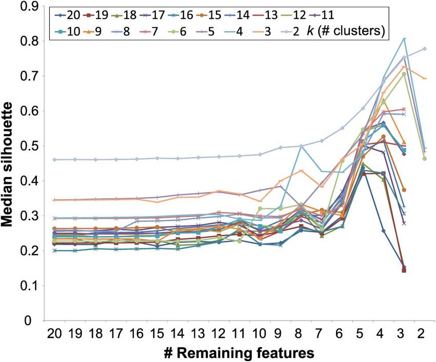
SEO ET AL.: IO WORKLOAD CHARACTERIZATION REVISITED: A DATA-MINING APPROACH                                                      3027

we thus focus on a generic framework to classify the workload       These approaches draw simple statistics on a limited set of
and include only spatial, temporal and volume aspects of IO         attributes (e.g., read/write ratios, IO size distribution, ran-
which can be analyzed without actually examining the con-           domness of IO), thus often failing to properly characterize the
tents of IO. In the cases in which the content examination is       correlations among different attributes.
feasible, considering content locality in workload characteri-          The workload analysis and classification can be used at
zation and classification may produce improved results.              different layers of the IO stack. Specifically, Li et al. proposed
    The advancement of NAND-based storage devices, which            to use a data-mining algorithm at the block device driver for
bear different physical characteristics from hard-disk-based        disk scheduling, data layout and prefetching [40]. Sivathanu
storage devices, calls for an entirely new way of characterizing    et al. proposed to embed the analysis function inside the file
IO workloads. In this paper, we revisit the issue of under-         system layer, which allows inference of the location of meta-
standing and identifying the essential constituents of modern       data region of the file system via the examination of the
IO workloads from the viewpoint of the emerging NAND-               workload access pattern [41]. Won et al. proposed to embed
based storage device. In particular, we aim at addressing the       the analysis function at the firmware of the storage device [30]
following specific questions: (i) What is the right clustering       and aimed at exploiting the workload characteristics to con-
algorithm for IO workload characterization’s sake? (ii) What        trol the internal behavior of the storage device (e.g., block
is the minimal set of features to effectively characterize the IO   allocation, the number of retries and error-correction coding).
workload? and (iii) How should we verify the effectiveness of           Sophisticated workload generators and measurement
the established classes? These issues are tightly associated        tools have been proposed for devising pattern-rich micro-
with each other and should be addressed as a whole. We              benchmarks [42]-[46]. These tools are useful for producing
apply a data-mining approach for this purpose. We perform a         arbitrary workload patterns in a fairly comprehensive man-
fairly extensive study for the comprehensiveness of the result:     ner. However, without the knowledge on essential patterns in
We examine eleven clustering algorithms and twenty work-            real-world workloads, it is not easy to generate appropriate IO
load features with tens of thousands of IO traces. We apply         workloads for accurate performance measurement.
both unsupervised and supervised learning approaches in a               The most important limitation out of all previous
streamlined manner. In particular, we apply unsupervised            approaches to IO workload characterization may be that these
learning first so that existing domain knowledge does not            approaches considered only HDDs as the storage device. The
bring any bias on establishing a set of traffic classes.             workload characterization for rotating media is relatively
    For SSDs, we can apply the proposed approach to intelli-        simple, because the dominant factor regarding the device
gent log-block management in hybrid mapping, victim selec-          performance is the seek overhead. Hence, characterizing
tion in garbage collection, and mapping-granularity decision        workloads in terms of sequentiality and randomness has
in multi-granularity mapping, although this paper does not          provided sufficient, even though not complete, ingredients
present the details of such applications. We further believe        to evaluate the performance of the file and storage stack.
that the proposed methodology can be applied to other types             Now that the NAND-based SSD is emerging as a strong
of storage devices for IO optimization.                             candidate for the replacement of the HDD, it is necessary to
    The rest of this paper is organized as follows: Section 2       characterize workloads in terms of more abundant attributes
presents prior work related to this paper, and Section 3 briefly     to accurately measure the performance of the file and storage
describes the overview of our work. Section 4 defines para-          stack. Recently, a workload generator called uFlip [47], [48]
meters and features for IO workload characterization. In            was proposed, which can generate more diverse workloads
Section 5, we select the most effective three features among        tailored for examining the performance of NAND-based
a total of twenty features and extract representative               SSDs. However, the essential IO patterns used in uFlip were
IO patterns using unsupervised learning techniques. In              not derived from real-world workloads. Thus, it is not known
Sections 6 and 7, we present a tree-based model of IO traces        whether these patterns are sound and complete ones for SSDs.
and a decision-tree-based pattern classification scheme,                 The objective of this work is to find the presentative
respectively. We conclude the paper in Section 8.                   patterns of IO workloads from NAND storage’s point of
                                                                    view. These patterns are to be exploited in designing various
                                                                    components of NAND-based storage device (e.g., address
                                                                    mapping, wear leveling, garbage collection, write buffer
2   BACKGROUND
                                                                    management, and other key ingredients).
2.1 Related Work
Data mining has been used for analyzing and evaluating
various aspects of computer systems. Lakhina et al. used            2.2 Flash Translation Layer (FTL)
entropy-based unsupervised learning to detect anomalies in          NAND flash memory has unique characteristics in contrast to
network traffic [28]. Won et al. applied an AdaBoost tech-           DRAM and HDDs. In particular, the flash translation layer
nique [29] to classify soft real-time IO traffic [30]. Park et al.   (FTL) [6]-[10] plays a key role in operating NAND-based
employed Plackett-Burgman designs to extract the principle          SSDs. The primary objective of FTL is to let existing software
features in file system benchmarks [31].                             recognize an SSD as a legacy, an HDD-like block device. FTL
   Regarding IO workload characterization, there have been          performs three main tasks: (i) FTL maintains a logical-address
empirical studies on characterizing file system access patterns      to physical-address translation table (i.e., address mapping),
and activity traces [32], [33]-[35]. Application-specific work-      (ii) FTL consolidates valid pages into a block so that invalid
load characterization efforts exist for web servers [36], [37],     pages can be reset and reused (i.e., garbage collection), and
decision support systems [38], and personal computers [39].         (iii) FTL evens out the wears of blocks by properly selecting
3028 IEEE TRANSACTIONS ON COMPUTERS, VOL. 63, NO. 12, DECEMBER 2014 physical blocks (i.e., wear leveling). To maximize IO perfor- workload analysis to data distribution. Inside recent SSDs, mance (latency and bandwidth) and to lengthen the NAND- the NAND flash chips are typically configured in multiple cell life time, FTL designers should carefully craft the channels, each of which consists of multiple ways. To exploit algorithms for selecting destination blocks for writing, for such a multi-channel/multi-way architecture, SSD controllers determining victim blocks for page consolidation, and for distribute write requests over multiple channels and ways. determining when to perform such consolidation. This can scatter data with locality over separate chips. If these The success of FTL lies on properly identifying incoming data are later modified, then the invalid data end up existing traffic and effectively optimizing its behavior. As a result, in multiple chips, which significantly deteriorates garbage- there have been various approaches to exploiting spatial, collection performance. To alleviate this issue, we need to temporal and volume aspects of IO workloads in the context keep data with locality in the same chip, to also exploit way of FTL algorithms. By allocating separate log blocks for interleaving. sequential and random workloads and managing them dif- One solution is to utilize the sequential random (SR) ferently, we can significantly reduce the overhead for merging pattern discovered by our approach (see Table 3 and Fig. 6). log blocks in hybrid mapping [6]. According to [7], we can We write sequential IOs to a single chip, thus maintaining significantly improve the log-block utilization and overall locality, and write random IOs to remaining chips in parallel, system performance by maintaining separate log-block thus achieving the effect of way interleaving. Going one step regions based upon the hotness of data. It was reported that further, we can divide sequential IOs into NAND-block-sized we can reduce the mapping table size by adopting different chunks and then write them to different chips in parallel. This mapping granularities, thus exploiting the IO-size distribu- will allow us to achieve interleaving effects, while still main- tion of incoming workloads [49]. Although these methods are taining locality (recall that the unit of erase is one NAND pioneering, they show rather unsatisfactory performance in block). This type of data distribution can make valid and classifying workloads, typically producing frequent misclas- invalid pages exist in different blocks by the effect of main- sification. We can conclude that there is a clear need for a more taining locality and eventually deliver positive effects on elaborate IO characterization framework for advancing SSD garbage collection. technology even further. 2.3 Applications of Workload Analysis to SSD 3 OVERVIEW We can utilize IO workload analysis results in multiple ways Fig. 1 shows the overall flow of our approach. Our objective is for optimizing the performance of NAND-based SSDs. We to find a set of representative patterns that can characterize IO present a few ideas here: enhancing write performance, re- workloads, and to propose a model that can later be used to ducing FTL mapping information, and improving garbage classify IO traces for class-optimized processing. In this paper, collection. The actual implementation of such ideas will be we first focus on defining such patterns of IO traces and part of our future work. constructing a model based on those patterns (depicted inside As elaborated in Section 4.2, we view and collect IO traces the dot-ted box labeled DESIGN TIME in Fig. 1). Then, we in the unit of the size of a write buffer, since this size show how to construct a simple but accurate classifier based corresponds to the largest size that an FTL can directly on this model. We can include this classifier in the firmware of manage for efficiently performing flash write operations. If a storage device and use it in runtime (depicted inside the box certain write patterns are found to be favorable for fast write labeled RUNTIME). operations (e.g., fully sequential patterns), then the FTL can We first collect a number of IO trace samples and represent reorder and merge the IO data pages stored temporarily in the each of them mathematically as a vector of various features. write buffer, transforming them into one of the patterns that Then, in the first phase of our approach, we analyze the can improve write performance. vectorized IO traces by clustering. Our hope is that, by Furthermore, we can significantly reduce the amount of applying an unsupervised learning approach, we can find FTL mapping information by workload pattern analysis. novel patterns of IO traces in addition to re-discovering Given that the capacity of SSDs is ever growing, using the known ones. We refer to the resulting clusters from this first conventional page-mapping scheme for terabyte-scale SSDs phase as preliminary IO trace patterns. would require gigabyte-scale mapping information. We Based on the clustering result from the previous step, we could use coarse-grained mapping, such as the block map- build a tree-based model that can represent characteristics of ping, but this would significantly degrade the random-write IO traces. Although clustering can give us an idea of what performance. For the data incurring few random writes (e.g., types of patterns appear in today’s IO workloads, we find multimedia data), we had better use coarse-grained mapping, that some of the preliminary patterns are redundant or have and for the data incurring frequent random writes (e.g., file little practical value. We streamline the preliminary clusters system metadata), we had better rely on fine-grained map- and define a new set of IO classes. We then represent them by ping, such as page mapping. If an FTL can distinguish and a tree structure, due to the hierarchical nature of the classes classify different data types automatically, then it can deter- of IO patterns. mine the optimal mapping granularity for each data type and We can apply the proposed model and classes of patterns minimize the amount of mapping information while mini- to classify incoming workloads efficiently. We can optimize mizing the decrease in IO performance. various SSD controller algorithms for each class of the IO Additionally, we can enhance the performance of garbage workloads so that the controller dynamically adapts its collection by applying the patterns discovered by IO behavior subject to the characteristics of incoming IO
SEO ET AL.: IO WORKLOAD CHARACTERIZATION REVISITED: A DATA-MINING APPROACH                                                     3029

Fig. 1. Overview of proposed approach.

(e.g., random vs. sequential, hot vs. cold, degree of correla-        indicate each BP by a solid circle. By definition, the
tions among IO accesses, garbage collection algorithms [13],          number of BPs is identical to that of segments.
[14], log block merge algorithms [6]-[9], and wear leveling        Continued point (CP): a CP is the start of a segment that
[11]-[13]).                                                           continues another earlier segment in the same trace. If the
                                                                      break point of a segment occurs at          , then        is a
                                                                      CP if                    and           > . For example, the
4    CHARACTERIZING IO TRACES                                         start point of segment 3 in Fig. 2b is a CP. The start points
4.1 Parameter Definitions                                              of the other segments are not.
An IO trace consists of multiple IO requests, each of which        Access length: this is the number of pages (or bytes) each IO
includes information on the logical block address (LBA) of the        request causes the IO device to read or write. For a segment
starting page, access type (read or write), and the number of         that consists of multiple IO requests, the segment length
pages to read or write. Fig. 2a shows an example trace that           is the sum of the access lengths of the component IO
consists of five IO requests. As shown in Fig. 2b, we can also         requests.
represent an IO trace as a series of LBA over pages. We can        Virtual segment: this comprises two or more segments that
denote an IO trace by function              , where is a set of       can form a continuous segment if we remove the inter-
page indices and a set of LBAs. We assume that or is a                vening pages between them. Two segments and form a
set of nonnegative integers.                                          virtual segment if                    and          > , where
   We can characterize an IO trace using the following para-             and are the last and first pages of and , respectively.
meters and definitions:                                                In Fig. 2b, segments 1 and 3 form a virtual segment.
Page size: we assume that the unit of a read or write is a page    Random segment: if a segment is smaller than a user-specified
    and that the size of each page is equal (e.g., 4 KB) for all      threshold and is not part of any virtual segment, then we
    traces.                                                           call this segment random. In Fig. 2b, if the user-specified
Trace size: the size of a trace is the total number of unique         threshold happens to be twice the length of segment 4,
    pages in the trace, or    .                                       then segment 2 is not random but segment 4 is.
Segment: a segment is a continuous LBA sequence in an IO           Up- and down-segment: if the start LBA of a segment is
    trace. Fig. 2b shows four segments. Note that multiple IO         greater than the BP of the previous segment, then we call
    requests can form a single segment. For example, segment          this segment an up-segment. (A down-segment is the
    1 in Fig. 2b consists of two IO requests: RQ1 and RQ2.            opposite.) In Fig. 2b, segments 2 and 4 are up-segments,
Break point (BP): a BP is the end of a segment. A BP occurs           whereas segment 3 is a down-segment.
    at page           if                       . In Fig. 2b, we
                                                                   4.2 IO Trace Data Collection
                                                                   We utilize a public data set [50], which consists of workloads
                                                                   from two web servers (one hosting the course management
                                                                   system at the CS department of Florida International Univer-
                                                                   sity, USA, and the other hosting the department’s web-based
                                                                   email access portal), an email server (the user ‘inboxes’ for the
                                                                   entire CS department at FIU) and a file server (an NFS server
                                                                   serving home directories of small research groups doing
                                                                   software development, testing, and experiments).
                                                                      In addition, we collect IO trace data from a system that has
                                                                   the following specifications: Intel Core 2 Duo E6750 CPU,
Fig. 2. Parameter definitions for characterizing IO traces.         2 GB 400 MHz DDR2 DRAM, Linux 2.6.35-28-generic, and a
3030 IEEE TRANSACTIONS ON COMPUTERS, VOL. 63, NO. 12, DECEMBER 2014
500 GB Seagate ST3500320AS HDD. To generate stride read TABLE 1
and write traces, we use IOzone version 3.308. We use the List of Features for Characterizing IO Traces
blktrace tool to collect IO traces during Windows 7 installa-
tions, text processing via MS Word version 2007, web surfing
using Google Chrome and MS Explorer and downloading
multimedia files.
The write buffer size of the SSD controller governs the size
of the observation window for classification. The length of the
IO trace in the clustering should be tailored to properly
incorporate the size of the write buffer. In our study, we
presume that the write buffer size is 32 MByte [51], [52], which
can hold 8,000 unique 4-KByte pages. This sets the length of
a trace to 8,000. In total, we generated 58,758 trace samples,
each of which has 8,000 unique pages.
To implement the IO trace analysis and data-mining algo-
rithms described in this paper, we use the R2010 b version of
the MATLAB programming environment (http://www.
mathworks.com) under 64-bit Windows 7.
4.3 Feature Definitions
Based on the above definitions, we characterize each IO trace
by the twenty features listed in Table 1. Features F1 and F2
indicate the length of a trace in terms of pages and time.
Feature F3 is the length of the longest segment. Features F4-F7 The features selected by backward elimination.
represent the total number of IO requests, BPs, CPs and non- The features used by tree-based model.
random segments. The other features are the ratios (F8-F10)
and basic statistics, such as arithmetic means (F11-F13), range possible classes is already determined, but as a supervised
(F14), and standard deviations (F16-F20) of other features. learning technique, it cannot discover novel patterns, unlike
Using these features, we transform each IO trace sample into a clustering.
vector of twenty dimensions for downstream analysis. That is, For clustering analysis of IO traces, we need to determine
we convert the input trace data into a matrix of 58,758 rows the set of features and the specific clustering algorithm used.
(recall that we used 58,758 traces in our experiments) and Since the set of best features differs by which clustering
twenty columns and then normalize this matrix so that every algorithm is used, we need to consider the two dimensions
column has zero mean and unit variance. at the same time for the optimal result. However, optimizing
We consider various features hoping that we can discover all of these simultaneously will be difficult due to the huge size
an important feature by exploring a variety of (combinations of search space. We thus determine the set of features by a
of) features, given that we do not know the best set of features feature selection procedure, with the clustering algorithm
for optimal IO characterization. However, due to the curse fixed. Then, with respect to the determined set of features,
of dimensionality [53] (or lack of data separation in high- we find the best clustering algorithm.
dimensional space), using too many features for data mining
could make it difficult to separate IO traces in the original 5.1 Evaluation Metric
feature space. Thus, we need to select a set of features for To assess different sets of features and clustering methods, we
better clustering results. In the next section, we will explain first need to establish a metric that can assess the quality of a
how to select a good set of features that yield a reasonable clustering result. Then, we search for the scheme that max-
clustering result. imizes this metric. In this paper, we use the silhouette value
[54], a widely used metric for scoring clustering results.
For a clustering result, we can assign each clustered sample
5 FINDING REPRESENTATIVE PATTERNS FROM IO a silhouette value. Then, we can represent the whole cluster-
TRACES BY CLUSTERING ing result by the median silhouette value of all clustered
samples. More specifically, we define , the silhouette value
Before building a model for classifying IO traces, we first
of sample , as follows [54]:
want to see what types of IO traces appear in storage systems.
The exact number of all possible patterns may be difficult to
determine, but we expect that we can find a small number of
representative patterns. To summarize the patterns of IO
traces in an automated fashion, we need a computational where represents the average distance of sample with
analysis tool that can handle a number of IO trace samples and all other samples within the same cluster, and denotes
find patterns therefrom. To this end, clustering is a perfect the lowest average distance to of the other clusters. By
fit, since clustering (as unsupervised learning) enables us to definition, a silhouette value can range from to .
find novel, previously unnoticed patterns beside known or represents the perfectly clustered sample, whereas indi-
expected ones. Classification is useful when the set of cates the opposite.SEO ET AL.: IO WORKLOAD CHARACTERIZATION REVISITED: A DATA-MINING APPROACH 3031
TABLE 2
List of Clustering Algorithms Used
this algorithm is , the number of clusters. For each value of
between 2 and 20, we perform the backward elimination
procedure and measure the median silhouette. Overall, the
highest peak is observed when and there remain three
Fig. 3. Backward elimination process for feature selection ( denotes the features. This means that clustering the trace data with respect
number of clusters). The median silhouette value is maximized with to these three features gives the highest silhouette. As shown
and three features.
in Table 1, these three features are F7 (the number of non-
random segments), F9 (the ratio of the number of CPs to that of
5.2 Feature Selection BPs), and F16 (the standard deviation of the starting LBAs of
The feature selection refers to a procedure to determine a set of IO requests).
features that yield the best clustering result. The feature
selection is computing intensive with the time complexity 5.3 Finding the Best Clustering Algorithm
exponential to the number of features. Among existing heu- Based on the three features determined in the previous step,
ristic approaches, we customize the backward elimination we cluster IO traces by ten different clustering algorithms
procedure [54], [55]. listed in Table 2. The selection covers most of the existing
The original backward elimination was developed for categories of clustering algorithms [29], [53], [54]: partitioning
supervised learning such as classification, in which we can (A1-A3), fuzzy (A3-A5), density-based (A6), and hierarchical
explicitly define classification error [29]. In such case, we start (A7-A10).
classification with the full set of features and measure the To adjust the input parameters of these clustering algo-
error. Then, we repeatedly drop the feature that decreases rithms, we rely on the silhouette metric. For instance, if one of
the error most significantly. In contrast, we cannot define the these clustering algorithms requires the number of clusters as
error in the current problem, which is an instance of unsuper- the input parameter (e.g., the parameter of the -means
vised clustering. Thus, we need to modify the original back- algorithm), we try multiple numbers and find the one that
ward elimination. yields the highest median silhouette value. For the hierarchi-
The procedure we use is as follows. The procedure is cal clustering algorithms that report a dendrogram (a hierar-
iterative, and in each iteration, we perform clustering by chical representation of samples) instead of flat clusters, we
dropping a feature at a time. Then we see if there is a feature use the common transformation technique that cuts the den-
that causes a change in the silhouette less than , a user- drogram at a certain height and group samples in each of the
specified threshold. If so, this means that this feature does not resulting sub-dendrograms into a cluster [54]. We find the
contribute to the clustering, and then we drop it. Otherwise, right cutting height by maximizing the median silhouette. For
we identify the feature that decreases the silhouette by the other clustering parameters (e.g., the parameter of DBSCAN
largest amount and remove it, since it hurts the clustering that sets the radius of the neighborhood that defines a “dense”
procedure by lowering the silhouette. (This corresponds to region), we also try different values of and use the one that
removing the feature that increases the classification error by gives the highest median silhouette value.
the largest amount in the supervised learning case.) We do not Fig. 4 shows the median silhouette values each of the
remove a feature that does not decrease the silhouette. clustering methods used reports. Refer to Table 2 for the
During backward elimination, we need to fix the clustering definition of the algorithm labels shown in the plot. For
algorithm used. In this paper, we use the -means clustering clustering, each algorithm uses only the three features (i.e.,
algorithm [54]. It runs fast and produces reasonable results F7, F9 and F16) determined in the previous backward elimi-
in many cases, although the -means algorithm sometimes nation step. For each clustering method, we try multiple
finds local optima only, as an example of the expectation- combinations of parameters as stated above, although Fig. 4
maximization algorithm [55]. shows only some of the results we obtained (including the
Fig. 3 shows how the median silhouette value varies during best ones) due to limited space.
the backward elimination process. For the sake of computa- According to Fig. 4, the partition-based algorithms (i.e., A1,
tional efficiency, we randomly sample 2,000 IO traces and A2 and A3) give the best results. The performance of the fuzzy
perform the backward elimination process on the selected IO algorithms and that of most of the hierarchical algorithms
traces. We set the threshold . The input parameter of follow next. The DBSCAN and single-linkage hierarchical3032 IEEE TRANSACTIONS ON COMPUTERS, VOL. 63, NO. 12, DECEMBER 2014
Fig. 4. Comparison of different clustering algorithms (see Table 2 for the
definitions of abbreviations).
algorithms show relatively low performance. In general,
DBSCAN can find more complex shapes of clusters than
partition-based algorithms can [53]. Nonetheless, the parti- Fig. 5. Samples of preliminary IO trace patterns found by unsupervised
clustering (features: F7, F9, F16; algorithm: -means). (a) (b) .
tioning algorithms produce better results in our experiments,
suggesting that IO traces tend to form clusters of rather simple
more types of clusters by increasing . Although the four
shapes. The single-linkage hierarchical algorithm is known to
clusters in Fig. 5a seem to represent some of the known IO
suffer from the problem of chaining [54] or the formation of
patterns well, there may be missing patterns for such a low
long, thin shape of clusters, which are often mere artifacts and
value of . According to our experiments, the median silhou-
fail to uncover the actual internal structure of samples. We
ette for is the highest for > when the -means
may attribute the lowest performance of the single-linkage
algorithm is used. For other types of clustering algorithms,
algorithm in our experiment to this problem. Based on this
we observe a slightly higher median silhouette for A8 with 17
result, we select the -means algorithm for downstream
clusters. However, the variation of the number of cluster
analysis due to its performance in terms of the silhouette and
members is rather high for this A8 case, meaning that some
its simplicity in implementation.
clusters have a large number of samples whereas others have
only a few. Thus, we decide to investigate the -means case for
5.4 Preliminary IO Trace Patterns . As expected, the clusters in Fig. 5b show more diverse
Fig. 5 shows two sets of clusters found by our approach from patterns. Cluster 1 corresponds to sequential IO patterns just
the 58,758 trace samples described in Section 4.2. Note that as Cluster 1 in the 4-cluster case does. Clusters 2 and 3 consist
each cluster represents a “preliminary IO trace pattern,” and of a long sequential pattern and a short random pattern
such patterns will become the grounds for constructing a tree- (similar to Cluster 3 in the 4-cluster case). Cluster 4 looks
based model in Section 6. To generate the result shown in the similar to Cluster 2 in Fig. 5. Clusters 9-12 represent random
figure, we use the -means clustering algorithm and the three patterns, resembling Cluster 4 in the 4-cluster case. Other
features determined by the backward elimination procedure. clusters seem to be related to strided patterns, similarly to
Due to limited space, we only show clusters for write opera- combinations of Clusters 3 and 4 in the 4-cluster case.
tions; we also found similar cluster formation for read
operations. 6 BUILDING A MODEL FOR CHARACTERIZING IO
Fig. 5a shows the representative clusters of write traces WORKLOADS
found from the clustering with . Recall that the median
silhouette is the highest when , as shown in Fig. 4. Among 6.1 Defining Classes of IO Traces
the known IO patterns (i.e., random, sequential and strided), Based on the preliminary patterns of IO traces found by
Clusters 1 and 4 in Fig. 5a represent the sequential and random clustering, we finalize a set of IO trace patterns. The prelimi-
IO patterns, respectively. Cluster 4 is a mixture of segments of nary clusters give us an idea of what types of patterns arise
short and moderate lengths. The IO requests in Cluster 2 in IO traces. We perform clustering without reflecting any
alternate between two LBA regions. In addition, Cluster 2 domain knowledge, in order not to prevent unexpected novel
seems to be related to the strided IO pattern. In Cluster 3, a patterns from appearing. In the second phase of our approach,
narrow range of LBAs are accessed except for a short period, we further streamline the clusters found in the previous step
during which distant addresses are accessed. Cluster 3 has and define a set of patterns. We can observe the following
both short and strided segments (in a magnified view, the from our clustering result summarized in Fig. 5:
longer segment consists of two alternating segments). O1: Segments play a role in shaping patterns. Depending on
Fig. 5b shows the clusters of write traces we found for the number of segments and their lengths, we can sepa-
. Our intention of using a larger value of is to examine rate patterns.SEO ET AL.: IO WORKLOAD CHARACTERIZATION REVISITED: A DATA-MINING APPROACH 3033
TABLE 3
Classes of IO Traces
We use the term ‘interleaved’ in lieu of ‘strided’ for the sake of avoiding
naming conflicts (using ‘strided’ would make the acronym of ‘strided full’
(SF) identical to ‘sequential full’).
Fig. 6. Sample IO traces for each of the nine classes.
gives us several key advantages over more complicated
alternatives (e.g., artificial neural networks and the support-
O2: There exist largely three categories of patterns corre- vector machine [53], [55]). We can use the constructed tree-
sponding to sequential, strided and random IO. The based model immediately as a pattern classifier used in the
sequential patterns include a small number of long firmware of a storage controller. Implementing a tree-based
segments, whereas the random patterns consist of many classifier is straightforward, and its running time overhead is
short segments. The strided patterns show somewhat typically negligible, since the classification using a tree model
regular structures of moderate segments and gaps consists of only a small number of comparison operations and
between them. does not entail any complex arithmetic operations.
O3: Each of the three basic patterns above has a few variants, Due to the stringent resource requirements of a consumer
giving 4 types of patterns in Fig. 5a and 12 types in product (e.g., cost, power consumption, and die size), it is not
Fig. 5b. practically feasible to use high-end microprocessors for SSD
O4: One such variant is the combined pattern that is a mixture controllers. A typical SSD controller uses an embedded pro-
of two or more basic patterns (e.g., a mixture of sequential cessor with a few hundred MHz of clock cycles without a
and strided). floating-point operation unit. The computational complexity
O5: Another variant is the pattern with a basic pattern of the classification algorithm used is of critical concern in the
corrupted by noise-looking short random accesses. SSD controller design and implementation. Employing a
Based on the above observations, we streamline the clus- more sophisticated classifier is likely to incur additional
ters in Fig. 5 and define 9 classes of IO traces. They are implementation complexity and runtime penalty with only
depicted in Fig. 6 with labels and descriptions listed in Table 3. marginal improvements.
Although most traces can be represented by (a combina- To construct a tree-based model, we need to determine, for
tion of) the three basic patterns (e.g. sequential, random, and each level of the tree, the criterion by which we make a
strided), we may encounter a trace that cannot be classified decision. For example, at the root level, we can group fully
into one of the predefined classes. Should such a trace arise, sequential patterns (SF) into the left node (excluding them
we can consider it as an ‘unknown’ class and skip the opti- from further consideration) and keep on classifying the
mized processing designed for the known classes. Later if the remaining patterns by going down to the right node. As the
frequency of observing unclassifiable traces increases, we can decision criterion at the root, a feature that can separate the SF
rerun the characterization and analysis flow to update the pattern and the rest would be useful in this example.
predefined classes. Note that the proposed methodology is The set of three features found by backward elimination
general and not limited to the nine classes currently presented. (i.e., F7, F9 and F16) was successful in discovering clusters in
the previous step of our approach, but we see some issues for
6.2 Representing Classes by Tree using this set of features as it is in the tree-based model
The classification of the 9 patterns shown in Fig. 6 is by design, construction. First, as shown in Fig. 7, the distributions of
hierarchical. That is, in the first level of the hierarchy, we can these three features are all skewed (the -th diagonal plot
classify IO traces into one of sequential, interleaved and shows the histogram of the -th feature; more explanation of
random classes. In the second level, each of these three classes this figure will follow shortly). This property might have
is further divided into three sub-classes, depending on more been useful in the clustering step, and probably this is why
detailed characteristics. Given that a tree can naturally repre- the set of these features was selected as the best combination of
sent a hierarchical structure, we build a tree-based model to features in backward elimination. However, using only those
represent the patterns of IO traces. Using a tree-based model features that have high skewness may produce severely3034 IEEE TRANSACTIONS ON COMPUTERS, VOL. 63, NO. 12, DECEMBER 2014
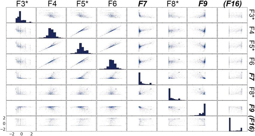
Fig. 7. Scatter-plot matrix [29], [56] of features (F7, F9, F16: selected by the backward elimination; F3, F5, F8: newly added during the tree-based
modeling; F16: not considered in the tree-based modeling).
unbalanced classification results. Some classes may have too with the root node. Then, we can find the SS class by applying
many samples, whereas others may have only a few. Second, F9 (the ratio of the number of CPs to that of BPs) at the second-
given that the tree-based model is to be implemented as part of level node. We can classify the other patterns by using the
the firmware of an IO system eventually, we should not ignore remaining features downward the tree, as shown in Fig. 8.
the computational overhead of obtaining features. In this Using the decision tree model shown in Fig. 8, we can
regard, the F16 feature (the standard deviation of the starting obtain the information on the quantitative appearance of each
LBAs of IO requests) is not ideal due to the need for calculating of the nine classes of IO traces listed in Table 3. For example,
the standard deviation. the SF patterns have F5 (the number of break points) values
To address these issues, we augment the set of features less than 4, whereas the SS patterns have F5 values between 4
selected from the clustering procedure as follows: First, we and 20, and F9 (the ratio of the number of continued points to
add F3 and F5 into the feature set in order to alleviate the that of break points) values less than 0.2.
skewness issue. Fig. 7 shows the scatter-plot matrix [29], [56]
of some of the 20 features defined in Table 1. In a scatter-plot
matrix, the plot drawn at location is the scatter plot
7 DECISION TREE FOR CLASSIFYING IO TRACES
showing the correlation between features and , and the -th Now that we have a tree-based model of IO traces, we can
diagonal plot is the histogram of feature presenting its construct a decision-tree-based classifier for classifying IO
distribution. In our data, F3-F6 are the top four features whose traces in runtime (Fig. 1). This section explains how to train
distributions resemble the normal distribution most closely. the classifier and validate it with real traces. Also, we compare
Among these, we drop F4 and F6 because their pairwise the proposed tree-based classifier with other existing state-
correlations with F5 are high (0.916 and 0.908, respectively), of-the-art classifiers in terms of classification accuracy and
and F5 can be used more conveniently to define the 9 classes running time. We also consider the impact of the length of
listed in Table 3 than these two. Second, instead of F16, we use trace samples on classification performance.
F8. We can justify this substitution on the following grounds.
Most of all, F8 is the last feature removed but F7, F9 and F16. 7.1 Training and Validating the Classifier
That is, if we had chosen four features by backward elimina- We collect labeled examples for each of the 9 classes from the
tion, not three, then the feature set would have had F7, F8, F9 58,758 trace samples. Following the standard procedure of
and F16. In addition, the two features that have the highest training and validating a classifier [53], we divide the class-
correlation with F16 turn out to be F7 and F8 (0.616 and 0.565, labeled samples into training and validation sets, train the
respectively); however, F7 is already in the feature set. Con- tree-based classifier using the training set and calculate the
clusively, replacing F16 by F8 should be a reasonable choice. classification error by the validation set. We perform this step
Based on this augmented set of features (F3, F5, F7, F8 via the 10-fold cross-validation [55]. In this procedure, we
and F9), we can build a tree-based model for the 9 classes divide labeled examples into 10 chunks of equal size, and train
defined in Table 3. First, we can separate the SF class by and validate the classifier 10 times. For each run, 9 of the 10
associating the decision regarding F5 (the number of BPs) chunks are used for training and the remaining one is forSEO ET AL.: IO WORKLOAD CHARACTERIZATION REVISITED: A DATA-MINING APPROACH 3035
Fig. 8. Proposed decision tree model of IO traces and examples.
validation in turn. We select the parameters of a classifier that 7.3 Performance Comparison
give the lowest validation error. Fig. 8 shows the resulting Fig. 9 compares the performance of different classifiers in
decision tree annotated with the threshold values for making terms of their classification error and running time. The
decisions at each node and some example patterns for each alternative classifiers tested include the support vector
class. machine (SVM) [55], the -nearest-neighbor classifier [29]
and the naïve Bayes classifier [53]. We utilize the WEKA
7.2 Class Distribution in Real Workloads machine learning package [29] for these sets of experiments.
To see how the 9 classes defined in Table 3 are distributed in Fig. 9a compares four alternative classification methods in
the real IO trace samples we collected, we classify the unla- terms of their accuracies relative to that of the tree-based
beled samples not used for training and validation. The set of classifier. The accuracy of the logistic-regression-based clas-
such samples are often described as the publication set. Table 4 sifier is the highest, and that of the naïve Bayes classifier is the
lists the breakdown of each of the 9 classes. Approximately lowest. The performance of the SVM, one of the most popular
half of all the IO trace samples are random patterns, while classifiers, is similar to that of the best one.
over 40% of them are interleaved patterns. Among the 9 Fig. 9b shows the running time required for classifying
classes defined in Table 3, the most frequently occurring 58,758 IO traces by the methods used for comparison.
pattern is the IM class, which consists of multiple strided
segments along with some random patterns. The RI class,
which has mostly random patterns with some strided pat- TABLE 4
Breakdown of 9 Classes in Real Trace Samples (See Table 3 for
terns, accounts for about 30% of trace samples. The chance of Definitions of Class ID)
seeing the fully sequential SF pattern is 2.58%, and summing
up all the percentages of SF, SS and SR classes yields 4.22%. It
would be exciting to see more sequential patterns, given that
some of the new storage systems can process sequential data
efficiently. It is notable that the strided patterns (the IF, IL and
IM classes) accounts for more than 40% altogether. Exploiting
such patterns would be beneficial in solid-state drives (SSDs)
that can assign each short segment to different channels
simultaneously, which can give a steep performance boost.
The fraction of fully random patterns (the RF class) is some-
what lower than expected.3036 IEEE TRANSACTIONS ON COMPUTERS, VOL. 63, NO. 12, DECEMBER 2014
a minimal feature set: the number of non-random segments,
the ratio of the number of continued points and the number of
break points, and the standard deviation of the starting LBAs
of IO requests. As IO classes, we establish nine essential
workload classes: three random, three sequential and three
mixture classes in legacy sense. Finally, we develop a classifi-
cation model of IO traces and construct a pattern classifier
based on the model for classifying IO traces in runtime. We
use a tree-based model that naturally fits the hierarchical
nature of workloads. Based on the model, we also develop
a decision tree for classifying IO trace in the storage stack of
the operating systems or the storage device firmware. An SSD
controller can effectively exploit this classification model to
characterize incoming workloads so that it can adaptively
apply it to essential tasks such as garbage collection, wear
leveling, and address mapping, tailoring these tasks to each
workload class. Later in our future work, we plan to develop
FTL techniques that can effectively utilize the classification
model proposed in this work.
ACKNOWLEDGMENTS
This work was supported in part by the National Research
Foundation of Korea (NRF) grant funded by the Korea
Fig. 9. Performance comparison of classifiers. (a) relative accuracy government (Ministry of Science, ICT and Future Planning)
(b) classification time.
[No. 2011-0009963 and No. 2012-R1A2A4A01008475] and
in part by the IT R&D program of Korea Evaluation Institute
As expected, the proposed method requires the least amount of Industrial Technology (KEIT) funded by the Korean
of time to complete the classification task. The advantage in government (Ministry of Trade, Industry and Energy)
running time obviously comes from the simplicity of the tree- [No. 10035202].
based model. When executed in an embedded CPU, the
proposed classifier would further widen the performance gap
among the other methods in terms of running time. As for the REFERENCES
accuracy in the embedded environment, we need further
[1] “SSD Prices Continue to Plunge,” http://www.computerworld.
studies in order to assess the effect of using fixed-point com/s/article/9234744/SSD_prices_continue_to_plunge, 2012.
operations for the classifiers under comparison. Still, we [2] “SSD Prices Are Low—and They’ll Get Lower,” http://arstechnica.
expect that the proposed approach would get affected the com/gadgets/2012/12/ssd-prices-are-low-and-theyll-get-lower/,
least, given its simplicity, compared with more sophisticated 2012.
[3] S.-W. Lee, B. Moon, C. Park, J.-M. Kim, and S.-W. Kim, “A Case for
classifiers such as the SVM, which often involves more com- Flash Memory SSD in Enterprise Database Applications,” Proc.
plicated arithmetic operations. ACM Special Interest Group on Management of Data (SIGMOD) Int’l
For the data we used, the training time of the proposed Conf. Management of Data, pp. 1075-1086, 2008.
[4] S.R. Hetzler, “The Storage Chasm: Implications for the Future of
classifier is faster than that of logistic regression but moder- HDD and Solid State Storage,” Proc. IDEMA Symp. What’s in Store for
ately slower than that of the other classifiers. However, in the Storage, the Future of Non-Volatile Technologies, 2008.
current context, it is needless to say that reducing classifica- [5] S.-W. Lee, B. Moon, and C. Park, “Advances in Flash Memory SSD
tion time is far more important than accelerating training. As a Technology for Enterprise Database Applications,” Proc. 35th ACM
Special Interest Group on Management of Data (SIGMOD) Int’l Conf.
lazy-learning method that defers all computation until clas- Management of Data, pp. 863-870, 2009.
sification [53], the -nearest-neighbor classifier does not need [6] S.-W. Lee, D.-J. Park, T.-S. Chung, D.-H. Lee, S. Park, and H.-J. Song,
any training but takes the largest running time, as presented in “A Log Buffer-Based Flash Translation Layer Using Fully-Associative
Fig. 9b, and requires storing all training data, which makes it Sector Translation,” ACM Trans. Embedded Computing Systems, vol. 6,
pp. 18-46, July 2007.
inappropriate in practice. Overall, the proposed approach [7] S. Lee, D. Shin, Y.-J. Kim, and J. Kim, “LAST: Locality-Aware Sector
outperformed the other classifiers in terms of classification Translation for NAND Flash Memory-Based Storage Systems,”
accuracy and time as well as the suitability of firmware Special Interest Group on Operating Systems (SIGOPS) Operating Sys-
tems Rev., vol. 42, pp. 36-42, Oct. 2008.
implementation. [8] J. Kim, J.M. Kim, S.H. Noh, S.L. Min, and Y. Cho, “A Space-Efficient
Flash Translation Layer for Compactflash Systems,” IEEE Trans.
Consumer Electronics, vol. 48, no. 2, pp. 366-375, May 2002.
8 SUMMARY AND CONCLUSION [9] H. Kwon, E. Kim, J. Choi, D. Lee, and S.H. Noh, “Janus-FTL: Finding
the Optimal Point on the Spectrum between Page and Block
We have described novel IO workload characterization and Mapping Schemes,” Proc. 10th ACM Int’l Conf. Embedded Software,
classification schemes based on the data mining approach. For pp. 169-178, 2010.
IO workload clustering, -means algorithm yields the best [10] A. Gupta, Y. Kim, and B. Urgaonkar, “DFTL: A Flash Translation
Layer Employing Demand-Based Selective Caching of Page-Level
silhouette value despite its simplicity. Among the twenty Address Mappings,” Proc. Int’l Conf. Architectural Support for Program-
features of the IO workload, we select three features to form ming Languages and Operating Systems (ASPLOS’09), pp. 229-240, 2009.SEO ET AL.: IO WORKLOAD CHARACTERIZATION REVISITED: A DATA-MINING APPROACH 3037
[11] Y.-H. Chang, J.-W. Hsieh, and T.-W. Kuo, “Endurance Enhancement [35] E. Riedel, M. Kallahalla, and R. Swaminathan, “A Framework for
of Flash-Memory Storage, Systems: An Efficient Static Wear Level- Evaluating Storage System Security,” Proc. USENIX Conf. File and
ing Design,” Proc. 44th ACM/IEEE Design Automation Conf. Storage Technologies (FAST), 2002.
(DAC’07), pp. 212-217, 2007. [36] M.F. Arlitt and C.L. Williamson, “Web Server Workload Character-
[12] L.-P. Chang, “On Efficient Wear Leveling for Large-Scale Flash- ization: The Search for Invariants (Extended Version),” Proc. ACM
Memory Storage Systems,” Proc. ACM Symp. Applied Computing, Special Interest Group on Performance Evaluation (SIGMETRICS),
pp. 1126-1130, 2007. pp. 126-137, 1996.
[13] N. Agrawal, V. Prabhakaran, T. Wobber, J.D. Davis, M. Manasse, [37] K. Krishna and Y. Won, “Server Capacity Planning under Web
and R. Panigrahy, “Design Tradeoffs for SSD Performance,” Proc. Traffic Workload,” IEEE Trans. Knowledge and Data Eng., vol. 11,
USENIX Ann. Technical Conf., pp. 57-70, 2008. no. 5, pp. 731-747, Sept./Oct. 1999.
[14] J.-W. Hsieh, L.-P. Chang, and T.-W. Kuo, “Efficient On-Line Identi- [38] B. Knighten, “Detailed Characterization of a Quad Pentium Pro
fication of Hot Data for Flash-Memory Management,” Proc. ACM Server Running tpc-d,” Proc. IEEE Int’l Conf. Computer Design,
Symp. Applied Computing, pp. 838-842, 2005. pp. 108-115, 1999.
[15] L.A. Barroso, K. Gharachorloo, and E. Bugnion, “Memory System [39] T. Harter, C. Dragga, M. Vaughn, A. Arpaci-Dusseau, and R. Arpaci-
Characterization of Commercial Workloads,” ACM SIGARCH Com- Dusseau, “A File Is Not a File: Understanding the I/O Behavior of
puter Architecture News, vol. 26, no. 3, pp. 3-14, 1998. Apple Desktop Applications,” Proc. Symp. Operating Systems Prin-
[16] J. Zedlewski et al., “Modeling Hard-Disk Power Consumption,” ciples (SOSP), pp. 71-83, 2011.
Proc. 2nd USENIX Conf. File and Storage Technologies, vol. 28, [40] Z. Li, Z. Chen, S.M. Srinivasan, and Y. Zhou, “C-Miner: Mining
pp. 32-72, 2003. Block Correlations in Storage Systems,” Proc. USENIX Conf. File and
[17] A. Riska and E. Riedel, “Disk Drive Level Workload Characteriza- Storage Technologies (FAST), pp. 173-186, 2004.
tion,” Proc. USENIX Ann. Technical Conf., pp. 97-103, 2006. [41] M. Sivathanu, V. Prabhakaran, F.I. Popovici, T.E. Denehy,
[18] S. Kavalanekar, B. Worthington, Q. Zhang, and V. Sharda, A.C. Arpaci-Dusseau, and R.H. Arpaci-Dusseau, “Semantically-
“Characterization of Storage Workload Traces from Production Smart Disk Systems,” Proc. USENIX Conf. File and Storage Technolo-
Windows Servers,” Proc. IEEE Int’l Symp. Workload Characterization gies (FAST), vol. 3, pp. 73-88, 2003.
(IISWC), pp. 119-128, 2008. [42] “Iometer,” http://www.iometer.org/, last accessed on Feb. 26, 2014.
[19] D. Molaro, H. Payer, and D. Le Moal, “Tempo: Disk Drive [43] N. Agrawal, A.C. Arpaci-Dusseau, and R.H. Arpaci-Dusseau,
Power Consumption Characterization and Modeling,” Proc. IEEE “Generating Realistic Impressions for File-System Benchmarking,”
13th Int’l Symp. Consumer Electronics (ISCE’09), pp. 246-250, 2009. Proc. 7th Conf. File and Storage Technologies, pp. 125-138, 2009.
[20] C. Park, P. Talawar, D. Won, M. Jung, J. Im, S. Kim, and Y. Choi, [44] E. Anderson, M. Kallahalla, M. Uysal, and R. Swaminathan,
“A High Performance Controller for NAND Flash-Based Solid State “Buttress: A Toolkit for Flexible and High Fidelity I/O Bench-
Disk (NSSD),” Proc. 21st IEEE Non-Volatile Semiconductor Memory marking,” Proc. 3rd USENIX Conf. File and Storage Technologies,
Workshop (NVSMW), pp. 17-20, 2006. pp. 45-58, 2004.
[21] Y. Lee, L. Barolli, and S.-H. Lim, “Mapping Granularity and Perfor- [45] “Filebench,” http://sourceforge.net/projects/filebench/.
mance Tradeoffs for Solid State Drive,” J. Supercomputing, [46] D. Anderson, “Fstress: A Flexible Network File Service Benchmark,”
vol. 65, pp. 1-17, 2012. Duke Univ., Technical Report TR-2001-2002, 2002.
[22] G. Wu and X. He, “Delta-FTL: Improving SSD Lifetime via Exploit- [47] L. Bouganim, B.T. Jonsson, and P. Bonnet, “uFLIP: Understanding
ing Content Locality,” Proc. 7th ACM European Conf. Computer Flash IO Patterns,” Proc. Classless Inter-Domain Routing (CIDR),
Systems, pp. 253-266, 2012. 2009.
[23] J. Kim, C. Lee, S. Lee, I. Son, J. Choi, S. Yoon, H.-U. Lee, S. Kang, [48] M. Bjorling, L. De Folgoc, A. Mseddi, P. Bonnet, L. Bouganim, and
Y. Won, and J. Cha, “Deduplication in SSDs: Model and Quantitative B. Jonsson, “Performing Sound Flash Device Measurements: Some
Analysis,” Proc. IEEE 28th Symp. Mass Storage Systems and Technolo- Lessons from uFLIP,” Proc. ACM Special Interest Group on Manage-
gies (MSST), pp. 1-12, 2012. ment of Data (SIGMOD) Int’l Conf. Management of Data, pp. 1219-1222,
[24] A. Gupta, R. Pisolkar, B. Urgaonkar, and A. Sivasubramaniam, 2010.
“Leveraging Value Locality in Optimizing NAND Flash-Based [49] G. Goodson and R. Iyer, “Design Tradeoffs in a Flash Translation
SSDs,” Proc. USENIX Conf. File and Storage Technologies (FAST), Layer,” Proc. HPCA Workshop on the Use of Emerging Storage and
pp. 91-103, 2011. Memory Technologies, Jan. 2010.
[25] Q. Yang and J. Ren, “I-CASH: Intelligently Coupled Array of SSD [50] R. Koller and R. Rangaswami, “I/O Deduplication: Utilizing
and HDD,” Proc. IEEE 17th Int’l Symp. High Performance Computer Content Similarity to Improve I/O Performance,” ACM Trans.
Architecture (HPCA), pp. 278-289, 2011. Storage (TOS), vol. 6, no. 3, p. 13, 2010.
[26] J. Ren and Q. Yang, “A New Buffer Cache Design Exploiting [51] S. Kang, S. Park, H. Jung, H. Shim, and J. Cha, “Performance Trade-
Both Temporal and Content Localities,” Proc. IEEE 30th Int’l Conf. Offs in Using NVRAM Write Buffer for Flash Memory-Based Storage
Distributed Computing Systems (ICDCS), pp. 273-282, 2010. Devices,” IEEE Trans. Computers, vol. 58, no. 6, pp. 744-758, June 2009.
[27] Y. Zhang, J. Yang, and R. Gupta, “Frequent Value Locality and [52] H. Kim and S. Ahn, “BPLRU: A Buffer Management Scheme for
Value-Centric Data Cache Design,” Proc. ACM SIGOPS Operating Improving Random Writes in Flash Storage,” Proc. 6th USENIX
Systems Rev., vol. 34, no. 5, 2000, pp. 150-159. Conf. File and Storage Technologies, pp. 1-14, 2008.
[28] A. Lakhina, M. Crovella, and C. Diot, “Mining Anomalies Using [53] J. Han, M. Kamber, and J. Pei, Data Mining: Concepts and Techniques.
Traffic Feature Distributions,” Proc. ACM Special Interest Group on Morgan Kaufmann Pub, 2011.
Data Communication (SIGCOMM), pp. 217-228, Aug. 2005. [54] P.N. Tan, M. Steinbach, and V. Kumar, Introduction to Data Mining.
[29] I.H. Witten and E. Frank, Data Mining: Practical Machine Learning Pearson Addison Wesley, 2006.
Tools and Techniques. Morgan Kaufmann, 2005. [55] E. Alpaydin, Introduction to Machine Learning. MIT Press, 2004.
[30] Y. Won, H. Chang, J. Ryu, Y. Kim, and J. Ship, “Intelligent Storage: [56] S. Few, Show Me the Numbers: Designing Tables and Graphs to
Cross-Layer Optimization for Soft Real-Time Workload,” ACM Enlighten, 2nd ed. Analytics Press, 2012.
Trans. Storage, vol. 5, no. 4, pp. 255-282, 2006.
[31] N. Park, W. Xiao, K. Choi, and D.J. Lilja, “A Statistical Evaluation of
the Impact of Parameter Selection on Storage System Benchmarks,”
Proc. 7th IEEE Int’l Workshop on Storage Network Architecture and
Parallel I/O (SNAPI), 2011.
[32] M.G. Baker, J.H. Hartman, M.D. Kupfer, K. Shirriff, and Bumjoon Seo is an advisory researcher with the
J.K. Ousterhout, “Measurements of a Distributed File System,” Proc. Emerging Technology Laboratory at Samsung
13th ACM Symp. Operating System Principles, pp. 198-212, 1991. SDS, Co., LTD., Seoul, Korea. His research inter-
[33] S. Gribble, G. Manku, D. Roselli, E. Brewer, T. Gibson, and E. Miller, ests include applications of data mining and
“Self-Similarity in File Systems,” Proc. Joint Int’l Conf. Measurement machine learning to storage systems design.
and Modeling of Computer Systems (SIGMETRICS), pp. 141-150, 1998.
[34] J. Ousterhout, H. Costa, D. Harrison, J. Kunze, M. Kupfer, and
J. Thompson, “A Trace-Driven Analysis of the Unix 4.2 bsd File
System,” Proc. 10th ACM Symp. Operating Systems Principles (SOSP),
pp. 15-24, 1985.You can also read