Monitoring of seasonal glacier mass balance over the European Alps using low-resolution optical satellite images
←
→
Page content transcription
If your browser does not render page correctly, please read the page content below
Journal of Glaciology (2016), 62(235) 912–927                                                                               doi: 10.1017/jog.2016.78
              © The Author(s) 2016. This is an Open Access article, distributed under the terms of the Creative Commons Attribution licence (http://creativecommons.
              org/licenses/by/4.0/), which permits unrestricted re-use, distribution, and reproduction in any medium, provided the original work is properly cited.

                  Monitoring of seasonal glacier mass balance over the European
                        Alps using low-resolution optical satellite images
                          VANESSA DROLON,1 PHILIPPE MAISONGRANDE,1 ETIENNE BERTHIER,1
                                       ELSE SWINNEN,2 MATTHIAS HUSS3,4
                           1
                            LEGOS, Université de Toulouse, CNRS, CNES, IRD, UPS, 14 av Edouard Belin, 31400 Toulouse, France
                      2
                        Remote Sensing Unit, Flemish Institute for Technological Research (VITO), Boeretang 200, 2400 MOL, Belgium
                          3
                           Department of Geosciences, University of Fribourg, Chemin du Musée 4, CH-1700 Fribourg, Switzerland
                     4
                       Laboratory of Hydraulics, Hydrology and Glaciology (VAW), ETH Zurich, Hönggerbergring 26, CH-8093 Zurich,
                                                                         Switzerland
                                        Correspondence: Vanessa Drolon

                            ABSTRACT. We explore a new method to retrieve seasonal glacier mass balances (MBs) from low-
                            resolution optical remote sensing. We derive annual winter and summer snow maps of the Alps during
                            1998–2014 using SPOT/VEGETATION 1 km resolution imagery. We combine these seasonal snow
                            maps with a DEM to calculate a ‘mean regional’ altitude of snow (Z) in a region surrounding a glacier.
                            Then, we compare the interannual variation of Z with the observed winter/summer glacier MB for 55
                            Alpine glaciers over 1998–2008, our calibration period. We find strong linear relationships in winter
                            (mean R2 = 0.84) and small errors for the reconstructed winter MB (mean RMSE = 158 mm (w.e.) a−1).
                            This is lower than errors generally assumed for the glaciological MB measurements (200–400 mm w.e.
                            a−1). Results for summer MB are also satisfying (mean R2 and RMSE, respectively, 0.74 and 314 mm w.
                            e. a−1). Comparison with observed seasonal MB available over 2009–2014 (our evaluation period) for
                            19 glaciers in winter and 13 in summer shows good agreement in winter (RMSE = 405 mm w.e. a−1) and
                            slightly larger errors in summer (RMSE = 561 mm w.e. a−1). These results indicate that our approach
                            might be valuable for remotely determining the seasonal MB of glaciers over large regions.
                            KEYWORDS: Alps, glaciers mass balance, NDSI, snow, SPOT/VEGETATION

              1. INTRODUCTION                                                                          technique requires heavy logistics, is time consuming and
              Glacier mass balance (MB) is highly sensitive to atmospheric                             moreover is subject to potential systematic errors (e.g.
              conditions and constitutes a direct and perceptible indicator                            Thibert and others, 2008). Glaciological MB measurements
              of climate change (Haeberli and Beniston, 1998). On a                                    are thus limited to a few easily accessible glaciers, unequally
              global scale, the mass loss of glaciers (apart from the                                  distributed around the globe: only about 150 glaciers among
              Greenland and Antarctica ice sheets) constitutes the major                               the world’s ∼200 000 glaciers are regularly monitored in the
              contribution to present sea-level rise (IPCC, 2013). For                                 field and present at least ten consecutive years of MB mea-
              example, over the well-observed 2003–2009 period,                                        surements (Pfeffer and others, 2014; Zemp and others, 2015).
              glacier mass loss was 259 ± 28 Gt a−1, representing about                                    Several remote sensing techniques are used to increase
              30 ± 13% of total sea-level rise (Gardner and others, 2013).                             data coverage of glacier mass change at a global scale.
              Between 1902 and 2005, glacier mass loss, reconstructed                                  One of them is the geodetic method, which consists of mon-
              by Marzeion and others (2015), corresponds to 63.2 ± 7.9 mm                              itoring glacier elevation changes by differencing multitem-
              sea-level equivalent (SLE). Glacier mass losses are projected                            poral DEMs. These DEMs can be derived from aerial
              to increase in the future and are expected to range between                              photos and/or airborne Light Detection and Ranging
              155 ± 41 mm SLE (for the emission scenario RCP4.5) and                                   (LiDAR) (Soruco and others, 2009; Abermann and others,
              216 ± 44 mm SLE (for RCP8.5) between 2006 and 2100                                       2010; Jóhannesson and others, 2013; Zemp and others,
              (Radić and others, 2014). Moreover, on continental surfaces,                            2013). However, the main limitation of airborne sensors is
              glacier behaviour strongly determines watershed hydrology:                               their geographic coverage, restricted to areas accessible
              glacier meltwater impacts on the runoff regime of mountain-                              with airplanes; some large remote areas such as High
              ous drainage basins and consequently on the availability of                              Mountain Asia can hardly be monitored. LiDAR data from
              the water resource for populations living downstream                                     the Ice Cloud and Elevation Satellite (ICESat) altimeter can
              (Huss, 2011). Many scientific, economic and societal                                     also provide information on glacier elevation changes, but
              stakes are thus related to glaciers (Arnell, 2004; Kaser and                             these data are too sparse to allow reliable monitoring of the
              others, 2010), hence justifying regular monitoring.                                      mass budget of individual glaciers (Kropáček and others,
                 Traditionally, the annual and seasonal glacier MBs are                                2014; Kääb and others, 2015). DEMs can also be derived
              measured using glaciological in situ measurements from                                   from medium-to-high resolution optical satellite images
              repeated snow accumulation surveys and ice ablation stake                                such as Satellite pour l’Observation de la Terre-High
              readings on individual glaciers, that are subsequently extra-                            Resolution Stereoscopic (SPOT5/HRS) images or radar satel-
              polated over the entire glacier area (Østrem and Brugman,                                lite images as done during the Shuttle Radar Topographic
              1991; Kaser and others, 2003). Nevertheless, this laborious                              Mission (SRTM). However, the vertical precision of these

Downloaded from https://www.cambridge.org/core. 16 Oct 2021 at 21:08:15, subject to the Cambridge Core terms of use.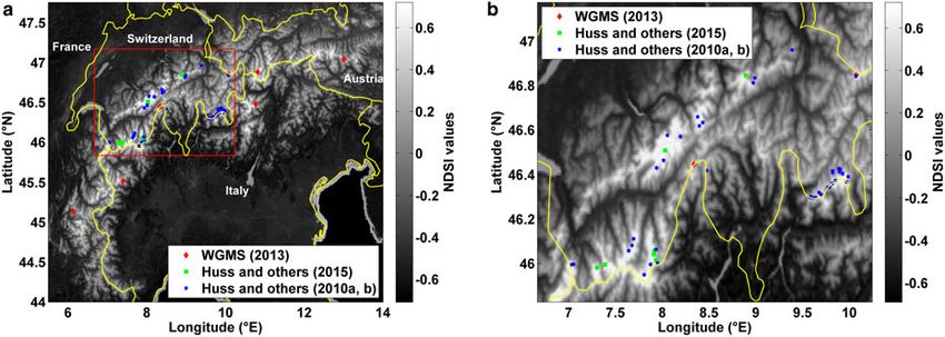
Drolon and others: Monitoring of seasonal glacier MB over the European Alps using low-resolution optical satellite images                               913

          DEMs (∼5 m) is such that it remains challenging to accurately                            consuming and require various datasets (meteorological
          estimate the MB of individual small to medium-sized glaciers                             data, remotely sensed data) that are not widely available.
          (glaciers < 10 km2) (Paul and others, 2011; Gardelle and                                     In this context, the consistent archive of optical SPOT/
          others, 2013). More recently, Worldview and Pléiades sub-                                VEGETATION (SPOT/VGT) images, spanning 1998–2014
          meter stereo images have been used to provide accurate                                   with a daily and nearly global coverage at 1 km resolution
          glacier topography with a vertical precision of ±1 m and                                 (Sylvander and others, 2000; Maisongrande and others,
          even ±0.5 m on gently sloping glacier tongues (Berthier                                  2004; Deronde and others, 2014), remains an unexploited
          and others, 2014; Willis and others, 2015). Nevertheless, re-                            dataset to estimate the year-to-year seasonal MB variations
          peatedly covering all glaciers on Earth with Worldview and                               of glaciers. Instead of detecting the exact physical snowline
          Pléiades stereo images would be very expensive given their                               altitude of a glacier as done in earlier studies, our new
          limited footprint for a single scene (e.g. 20 km × 20 km for                             method focuses on monitoring a ‘mean regional’ seasonal
          Pléiades). Due to DEM errors and uncertainties in the                                    altitude of snow (Z), in a region surrounding a glacier,
          density value for the conversion from volume change to                                   during summer (from early May to the end of September)
          mass change (Huss, 2013), this method currently provides                                 and winter (from early October to the end of April). The inter-
          MB at a temporal resolution typically, of 5–10 a. This does                              annual dynamics of this altitude Z, estimated from SPOT/
          not provide an understanding of glacier response to climatic                             VGT images, is then compared with the interannual variation
          variations at seasonal and annual timescales (Ohmura,                                    of observed seasonal MBs (derived from direct glaciological
          2011).                                                                                   measurements), available continuously every year over
              An alternative method to estimate the MB change of a                                 1998–2008, for 55 glaciers in the Alps (WGMS, 2008,
          glacier is based on the fluctuations of the glacier equilibrium                          2012, 2013; Huss and others, 2010a, b, 2015). The perform-
          line altitude (ELA) (Braithwaite, 1984; Kuhn, 1989; Leonard                              ance of the 55 individual linear regressions between Z and
          and Fountain, 2003; Rabatel and others, 2005). The ELA is                                MB are analysed in terms of the linear determination coeffi-
          the altitude on a glacier that separates its accumulation                                cient R2 and the RMSE. For each of the 55 regressions, we
          zone, where the annual MB is positive, from its ablation                                 then perform a cross-validation of the temporal robustness
          zone, where the annual MB is negative (Ohmura, 2011;                                     and skill of the regression coefficients. For all 55 glaciers, sea-
          Rabatel and others, 2012). The ELA and annual glacier-                                   sonal MBs are then calculated outside of the calibration
          wide MB are strongly correlated. Early studies have shown                                period, i.e. each year of the 2009–2014 interval. A validation
          that the ELA can be efficiently approximated by the snowline                             is realized for some glaciers with observed seasonal MB over
          altitude at the end of the ablation season (i.e. at the end of the                       2009–2014. Finally, we discuss the possible causes of differ-
          hydrological year) on mid-latitude glaciers (LaChapelle,                                 ences in the results between seasons, between glaciers and
          1962; Lliboutry, 1965). The snowline altitude measured at                                present the limits and perspectives of our methodology.
          the end of the ablation season thus constitutes a proxy for es-
          timating the annual MB. This method has been applied to
          glaciers located in the Himalayas, Alaska, Western North                                 2. DATA
          America, Patagonia and the European Alps amongst others,
          using aerial photographs or optical remote sensing images                                2.1. Satellite data
          from Landsat and MODIS (Ostrem, 1973; Mernild and                                        This study uses optical SPOT/VGT satellite images provided
          others, 2013; Rabatel and others, 2013; Shea and others,                                 by two instruments: VEGETATION 1 from April 1998 to the
          2013). However, the Landsat temporal resolution of 16 d                                  end of January 2003 (VGT 1 aboard the SPOT 4 satellite
          can be a strong limitation for accurately studying the dynam-                            launched in March 1998), and VEGETATION 2 from
          ics of snow depletion, especially in mountainous regions                                 February 2003 to the end of May 2014 (VGT 2 aboard the
          with widespread cloud coverage (Shea and others, 2013);                                  SPOT 5 satellite launched in May 2002). The instruments
          and the methodologies used with MODIS (available since                                   provide a long-term dataset (16 a) with accurate calibration
          2000) to detect ELA often require complex algorithms imply-                              and positioning, continuity and temporal consistency. The
          ing heavy classification (Pelto, 2011; Shea and others, 2012;                            SPOT/VGT sensors have four spectral bands: the blue B0
          Rabatel and others, 2013).                                                               (0.43–0.47 μm), the red B2 (0.61–0.68 μm), the Near Infra-
              Unlike the above-mentioned techniques, only a few                                    Red B3 (0.78–089 μm) and the Short Wave Infra-Red SWIR
          recent studies have focused on retrieving seasonal glacier                               (1.58–1.75 μm). Both sensors provide daily images of
          MBs (Hulth and others, 2013; Huss and others, 2013).                                     almost the entire global land surface with a spatial resolution
          Seasons are in fact, more relevant timescales to better under-                           of 1 km, in a ‘plate carree’ projection and a WGS84 datum
          stand the glacier response to climate fluctuations, allowing                             (Deronde and others, 2014). In this study, we used the
          the partitioning of recent glacier mass loss between                                     SPOT/VGT-S10 products (10-daily syntheses) freely avail-
          changes in accumulation (occurring mainly in winter) and                                 able between April 1998 and May 2014 (http://www.vito-
          changes in ablation (occurring mainly in summer), at least                               eodata.be/PDF/portal/Application.html#Home). The SPOT/
          in the mid- and polar latitudes (Ohmura, 2011). Hulth and                                VGT-S10 products, processed by Vlaamse Instelling voor
          others (2013) combined melt modelling using meteorologic-                                Technologisch Onderzoek (VITO), result from the merging
          al data and snowline tracking measured in the field with GPS                             of data strips from ten consecutive days (three 10-d syntheses
          to determine winter glacier snow accumulation along snow-                                are made per month) through a classical Maximum Value
          lines. Huss and others (2013) calculated the evolution of                                Composite (MVC) criterion (Tarpley and others, 1984;
          glacier-wide MB throughout the ablation period also by com-                              Holben, 1986). The MVC technique consists of a pixel-by-
          bining simple accumulation and melt modelling with the                                   pixel comparison between the 10-daily Normalized
          fraction of snow-covered surface mapped from repeated                                    Difference Vegetation Index (NDVI) images. For each pixel,
          oblique photography. Both methods have been applied for                                  the maximum NDVI value at top-of-atmosphere is picked.
          only one or two glaciers, and a few years as they are time-                              This selection allows minimizing cloud cover and aerosol

Downloaded from https://www.cambridge.org/core. 16 Oct 2021 at 21:08:15, subject to the Cambridge Core terms of use.
914 Drolon and others: Monitoring of seasonal glacier MB over the European Alps using low-resolution optical satellite images
contamination. Due to atmospheric effects, an atmospheric but with discontinuous data. At the time of access to the data-
correction is applied to the VGT-S10 products (Duchemin base, continuous seasonal MB time series were only avail-
and Maisongrande, 2002; Maisongrande and others, 2004) able for seven glaciers since 1998 (labelled ‘source 1’ in
based on a modified version of the SMAC (Simple Method Table S1).
for the Atmospheric effects) code (Rahman and Dedieu, The second MB dataset provided by Huss and others
1994). The SPOT/VGT-S10 Blue, Red and SWIR spectral (2015) is derived from recently re-evaluated glaciological
bands have been gathered from 1 April 1998 to 31 May measurements. For seven Swiss glaciers (labelled ‘source 2’
2014, over a region including the Alps and stretching from in Table S1), long-term continuous seasonal MB series from
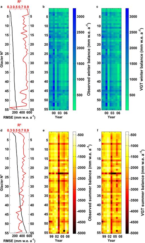
43 to 48.5°N and from 4 to 17°E (Fig. 1). 1966 (at least) to 2014 are inferred from point measurements
The terrain elevation over the studied region has been extrapolated to the entire glacier using distributed modelling,
extracted from the SRTM30 DEM, derived from a combin- with year-to-year variability directly given by the in situ
ation of data from the SRTM DEM (acquired in February measurements.
2000) and the U.S. Geological Survey’s GTOPO30 dataset The third MB dataset, composed of 41 Swiss glaciers, is a
(Farr and Kobrick, 2000; Werner, 2001; Rabus and others, comprehensive set of field data homogenized using distribu-
2003). The SRTM30 spatial resolution is 30 arcsec (∼ 900 m) ted modelling, with year-to-year variation constrained by
and the geodetic reference is the WGS84 EGM96 geoid. meteorological data (Huss and others, 2010a, b). The season-
The DEM has been resampled using the nearest-neighbour al MB time series of 21 glaciers covering 30% of the total
method to a 1 km spatial resolution in order to match the glacier area of Switzerland (labelled ‘source 3a’ in
resolution of the S10 SPOT/VGT images. Table S1), are available for each year of the 1908–2008
period (Huss and others, 2010a). For 20 other glaciers
located in the southeastern Swiss Alps (labelled ‘source 3b’
2.2. Glacier MB data in Table S1), seasonal MB time series are provided each
Glacier-wide winter and summer MB data of 55 different gla- year from 1900 to 2008 (Huss and others, 2010b). The con-
ciers are used in this study (Table S1 in the Supplementary tinuous seasonal MB series of these 41 glaciers are derived
Material; Fig. 1), covering a total area of ∼400 km2, corre- from three different data sources:
sponding to 19% of the 2063 km2 glacier area in the Alps
(1) Geodetic data of volume change for periods of four
(Pfeffer and others, 2014). Winter MB (Bw) is measured
to ∼ 40 a; three to nine DEMs have been used for each
through to the end of April. Summer MB (Bs) is the difference
glacier since 1930, mostly originating from aerial photo-
between annual MB determined at the end of the ablation
grammetry or terrestrial topographic surveys for the first
period (end of September) and winter MB (Thibert and
DEM.
others, 2013). Winter MB corresponds to the snow/ice
(2) (Partly isolated) in situ measurements of accumulation
mass accumulated during the winter season (from
and ablation for about half of the glaciers; they were
Octoberyear−1 to Aprilyear of measurement); thereafter, for more
used to constrain MB gradients and winter accumulation.
clarity, Bw_obs refers to the winter MB measured in April of
(3) Distributed accumulation and temperature‐index melt
the year of measurement and Bs_obs to the summer MB mea-
modelling (Hock, 1999; Huss and others, 2008) forced
sured in September of the year of measurement.
with meteorological data of daily mean air temperature
The different MB datasets all start before 1998. However,
and precipitation, recorded at various weather stations
as we later compare these MB data with SPOT/VGT snow
close to each of the glaciers. The model is constrained
maps available since April 1998, we used seasonal MB
by ice volume changes obtained from DEM differencing
only after 1998.
and calibrated with in situ measurements when avail-
The first MB dataset is composed of direct glaciological
able. Huss and others (2008) provide more details on
measurements provided by the World Glacier Monitoring
the model and calibration procedure.
Service (WGMS, 2013). Seasonal MB of 44 Austrian,
French, Italian and Swiss glaciers of the European Alps are In order to have the most complete set of continuous inter-
available between 1950 and 2012 (for the longest series) annual MB data to calibrate our method, we chose to
Fig. 1. Map of the mean NDSI for the period 1998–2014, over the European Alps, and location of the studied glaciers with MB balance
measurements (sources 1–3; Table S1). (a) Entire study area. (b) Enlargement of the studied area (red rectangle in (a)).
Downloaded from https://www.cambridge.org/core. 16 Oct 2021 at 21:08:15, subject to the Cambridge Core terms of use.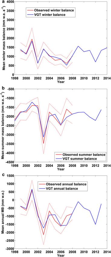
Drolon and others: Monitoring of seasonal glacier MB over the European Alps using low-resolution optical satellite images                            915

          combine MB time series from all sources (1, 2, 3a, b) over the                           A different (and more standard) formulation of the NDSI is
          same period. Since 41 glaciers (annotated 3a, b in Table S1)                             used for the MODIS sensor and calculated only with the
          provide continuous seasonal MB until 2008, the calibration                               red B0 channel and the SWIR (Xiao and others, 2001). Our
          period extends until 2008. As we later compare MB data                                   entire methodology was also tested with this standard NDSI
          with SPOT/VGT images provided since April 1998, 1999–                                    but led to results of inferior quality (not shown).
          2008 constitutes the winter calibration period and 1998–                                     Clouds have a spectral signature similar to snow and they
          2008 the summer calibration period. In total, 55 glaciers                                can be misclassified as snow, especially at the edge of the
          with 10 a of winter MB (Bw_obs) over 1999–2008, and 11 a                                 snow pack. We apply a cloud mask proposed by
          of summer MB (Bs_obs) over 1998–2008 have thus been                                      Dubertret, (2012) (and refer to as D-12 cloud mask below)
          used to calibrate our approach. Coordinates, median eleva-                               in order to flag cloudy pixels and to avoid overestimating
          tion and glacier area are available for all 55 glaciers                                  snow coverage. This algorithm, based on various reflectance
          (Table S1).                                                                              bands threshold tests, has been adapted to SPOT / VGT
              Furthermore, seasonal MBs are also available for some of                             images from different cloud masks initially created for
          these 55 glaciers outside the calibration period (2009–2014,                             higher resolution imagery. It corresponds to the crossing of
          i.e. the end of the period covered by SPOT/VGT data). In                                 Sirguey’s cloud mask (developed for MODIS sensor)
          winter, 66 additional Bw_obs data are available in total for                             (Sirguey and others, 2009) and of Irish and Zhu’s cloud
          19 glaciers over 2009–2014 and in summer, 49 Bs_obs mea-                                 masks, both developed for the Landsat sensor (Irish, 2000;
          surements are available for 13 glaciers over 2009–2013                                   Zhu and Woodcock, 2012). When compared with other
          (summer 2014 is not covered by SPOT/VGT) (WGMS,                                          classical cloud detection algorithms (e.g. Berthelot, 2004),
          2013; Huss and others, 2015).                                                            the D-12 cloud mask performs the best cloud identification,
              Errors associated with Bw_obs and Bs_obs are not provided                            along with Lissens and others (2000) cloud mask.
          individually per glacier. Zemp and others (2013) find an                                 However, Dubertret (2012) concluded that the D-12 cloud
          average annual random error of 340 mm w.e. a−1 for 12 gla-                               mask is more conservative than that of Lissens and others
          ciers with long-term MB measurements. Huss and others                                    (2000) and allows detection of more-snow covered pixels
          (2010a) have quantified the uncertainty in glacier-wide                                  (by flagging less clouds). We therefore choose to apply the
          winter balance (see Supplementary Information in their                                   cross-cloud mask on the S10 syntheses, which are compo-
          paper) as ±250 mm w.e. a−1. This number is not directly ap-                              sites of the S1 daily images pixels over 10 d.
          plicable to all glaciers (depending on the sampling), but to                                 A temporal interpolation is then computed for the ‘cloudy’
          most of them. Systematic errors associated with in situ glacio-                          pixels when possible. If a pixel is detected as cloudy in a S10
          logical MBs are expected to be within 90–280 mm w.e. a−1 if                              synthesis, its value is replaced by the mean of the same pixel
          cautious measurements are realized with sufficient stake                                 value in the previous synthesis (S10t−1), and in the next one
          density (Dyurgerov and Meier, 2002), but they are generally                              (S10t+1) if these pixels are not cloudy. If they are, we
          assumed to range between 200 and 400 mm w.e. a−1 for one                                 compute the mean of the S10t−2 and the S10t+2 synthesis
          glacier (Braithwaite and others, 1998; Cogley and Adams,                                 pixel values. In order to produce maps of winter/summer
          1998; Cox and March, 2004). In this study, we consider an                                NDSI, we average all 10-d NDSI syntheses included
          error (noted Eobs) of ±200–400 mm w.e. a−1 for observed MB.                              between 1 October and 30 April for each winter of the
                                                                                                   1999–2014 period, and between 1 of May and 30 of
                                                                                                   September for each summer of the 1998–2013 period.
          3. METHODS
          3.1. Cloud filtering and temporal interpolation of the                                   3.2. Calibration
          snow cover maps                                                                          We first superimpose each interannual mean seasonal NDSI
          Snow discrimination is based on its spectral signature, which                            map derived from SPOT / VGT for the period 1998–2014 on
          is characterized by a high reflectance in the visible and a                              the SRTM30 DEM. Then, considering different sized of
          high absorption in the SWIR wavelength. Consequently,                                    square windows varying from 5 to 401 km side lengths
          the Normalized Difference Snow Index (NDSI) first intro-                                 (with steps of 2 km) of P × P pixels and centred on each
          duced by Crane and Anderson (1984) and Dozier (1989)                                     glacier, we derive the altitudinal distribution of the mean sea-
          for the Landsat sensor, defined as a band ratio combining                                sonal NDSI. For each glacier, we thus obtain the interannual
          the visible (green) and SWIR Landsat bands, constitutes a                                dynamics of the NDSI altitudinal distribution within different
          good and efficient proxy to map the snow cover with                                      Windows of Snow Monitoring (WOSM) sizes surrounding
          optical remote sensing. The NDSI has since been widely                                   the glacier (16 curves; Fig. 2). The WOSM side lengths
          used with different sensors (e.g. Fortin and others, 2001;                               tested are always odd numbers for the glacier to be situated
          Hall and others, 2002; Salomonson and Appel, 2004). The                                  in the central pixel of the square window. Then for each
          NDSI value is proportional to the snow cover rate of the                                 WOSM size, from the intersection between a NDSI value
          pixel and allows a monitoring of the spatial and temporal                                (varying from 0.2 to 0.65, with a step of 0.01) and each sea-
          snow cover variations (Chaponnière and others, 2005). In                                 sonal curve of the NDSI altitudinal distribution, a ‘mean re-
          this study, we build an NDSI adapted to the SPOT/VGT                                     gional’ altitude of snow (Z) can be deduced each year,
          sensor (without green channel), inspired by Chaponnière                                  from 1998 to 2014. We do not focus on detecting the
          and others (2005). This modified NDSI is computed from                                   exact physical snowline elevation of the glacier at the end
          the mean of the red B0 and blue B2 channels (to recreate                                 of the melt season to estimate annual MB, as done in previous
          an artificial green band) and from the SWIR:                                             studies (e.g. Rabatel and others, 2005). In fact, the SPOT /
                                                                                                   VGT 1-km resolution is not adapted to monitor the snowline
                                          ðB0 þ B2Þ=2  SWIR                                       elevation and its high spatial variability. Moreover, the snow-
                               NDSI ¼                        :                           ð1Þ
                                          ðB0 þ B2Þ=2 þ SWIR                                       line approach does not allow us to retrieve seasonal MB,

Downloaded from https://www.cambridge.org/core. 16 Oct 2021 at 21:08:15, subject to the Cambridge Core terms of use.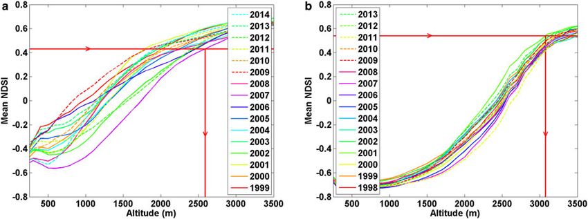
916                           Drolon and others: Monitoring of seasonal glacier MB over the European Alps using low-resolution optical satellite images

              Fig. 2. Altitudinal distribution of NDSI for each year since 1998. The NDSI has been averaged in a square window centred on Griesgletscher,
              central Swiss Alps. The red horizontal line represents the NDSI value from which the mean regional snow altitude Z (represented by the red
              vertical line) is inferred for each year. (a) Winter NDSI over 1999–2014 (WOSM size: 367 × 367 km²; NDSI value: 0.43). (b) Summer NDSI
              over 1998–2014 (WOSM size: 117 × 117 km²; NDSI value: 0.54).

              because at the end of the accumulation period (end of April/                                 To summarize, for each glacier, a linear regression is com-
              beginning of May in the Alps), the entire glacier is generally                           puted for each plausible NDSI value and all WOSM sizes.
              covered by snow. For these reasons, we aim at estimating for                             Following some initial tests on a subset of the 55 glaciers,
              winter and for summer a statistical mean regional altitude of                            the interval of plausible NDSI values is set to [0.2–0.65].
              snow in a region surrounding a glacier. Finally, for each                                This NDSI range has also been chosen to include the refer-
              WOSM size and each NDSI value that are tested, we                                        ence NDSI value of 0.4 commonly accepted to classify a
              compute a linear regression between the mean regional                                    pixel as snow-covered (and associated with a pixel snow
              snow altitudes Z and the observed MBs (Fig. 3), over the cali-                           cover rate of 50%) (Hall and others, 1995, 1998;
              bration period (1999–2008 for winter, 1998–2008 for                                      Salomonson and Appel, 2004; Hall and Riggs, 2007;
              summer). This linear regression allows an interannual estima-                            Sirguey and others, 2009). Then, for each glacier, and each
              tion of the glacier’s seasonal MB, as a function of Z inferred                           size of WOSM tested, the seasonal NDSI value optimizing
              from SPOT/VGT, as written in the linear equation (general-                               the RMSEw/s_cal is selected. This NDSI value adjustment for
              ized for both seasons):                                                                  each individual site (and each season) allows a better adap-
                                  Bw=s         ¼ αw=s × Zw=s þ β w=s :                       ð2Þ       tation to the glacier-specific environment (e.g. local land
                                         VGT
                                                                                                       cover type, local topography, etc.).
              Bw/s_VGT is the winter/summer MB estimated for the year y.                                   After adjusting the NDSI value, the size of the P × P pixels
              Zw/s is the winter/summer ‘mean regional’ altitude of snow;                              WOSM surrounding each glacier is also adjusted for each
              the slope coefficient αw/s expressed in mm w.e. a−1 m−1                                  glacier and each season. Here again, the WOSM size minim-
              represents the sensitivity of a glacier winter/summer MB                                 izing the mean RMSEw/s_cal is selected (Table S1 in
              towards Zw/s and βw/s is the winter/summer intercept term                                Supplementary Material). The WOSM side lengths tested
              expressed in mm w.e. a−1.                                                                are always odd numbers for the glacier to be situated in the
                 Coefficients of determination R2w/s and RMSEw/s_cal are                               central pixel of the window. A mandatory condition for the
              computed to assess the quality of the regression over the cali-                          WOSM size selection is the continuity of the NDSI altitudinal
              bration period for each season.                                                          curves, given the 100 m altitudinal step. The cost function f

              Fig. 3. Observed (a) winter and (b) summer MB of Griesgletscher, central Swiss Alps, as a function of the mean regional snow altitude Z for
              each year of the calibration period represented by coloured dots. Dashed thin lines represent the 95% confidence intervals for linear
              regression (solid line).

Downloaded from https://www.cambridge.org/core. 16 Oct 2021 at 21:08:15, subject to the Cambridge Core terms of use.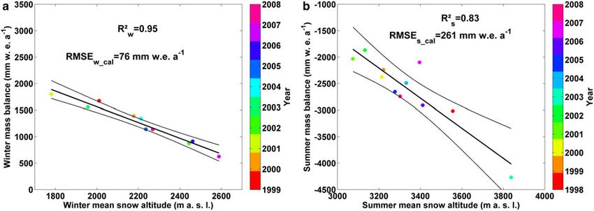
Drolon and others: Monitoring of seasonal glacier MB over the European Alps using low-resolution optical satellite images 917
optimizing the RMSEw/s_cal for each glacier is thus: of the error RMSEw/s_cross defined as:
0sffiffiffiffiffiffiffiffiffiffiffiffiffiffiffiffiffiffiffiffiffiffiffiffiffiffiffiffiffiffiffiffiffiffiffiffiffiffiffiffiffiffiffiffiffiffiffiffiffiffiffiffiffiffiffiffiffiffiffiffiffiffiffiffiffiffiffiffiffiffiffiffiffi
PN 1
f ðNDSI ; WOSM ; αw=s ; β w=s Þ ¼
ðBw=s VGT cross; y Bw=s obs; y Þ2
0sP ffiffiffiffiffiffiffiffiffiffiffiffiffiffiffiffiffiffiffiffiffiffiffiffiffiffiffiffiffiffiffiffiffiffiffiffiffiffiffiffiffiffiffiffiffiffiffiffiffiffiffiffiffiffiffiffiffiffiffiffiffiffi1 ¼@ A:
y¼1
RMSEw=s cross
N
y¼1 ðBw=s VGT y Bw=s ref y Þ A
2 ð3Þ N
min@ :
N ð4Þ
NDSI* and WOSM* are respectively the NDSI value and the We then estimate the skill score of the linear regression as
WOSM side length minimizing the RMSEw/s_cal. Allowing the 2
RMSEw=s
adjustment of both the NDSI value and the WOSM size is a SSw=s ¼ 1
cross
; ð5Þ
2
RMSEw=s
means to select an optimized quantity of snow-covered ref cross
pixels (where snow dynamics occurs) that are less affected
by artefacts such as residual clouds, aerosols and/or direc- where RMSEw/s_obs_cross is the mean square error of a refer-
tional effects. Changing NDSI value is a means to scan the ence model. As the reference model, we determine
terrain in altitude, while changing the windows size is a Bw/s_ref_cross,y for each year y by averaging the observed MB
means to scan the terrain in planimetry. values leaving out Bw/s_obs,y, (allowing that Bw/s_ref_cross,y is in-
Consequently, for each glacier, a unique ‘optimized’ dependent of the observed Bw/s_obs,y). The skill score can be
linear regression (regarding the parameters α and β) allows interpreted as a parameter that measures the correlation
us to estimate the seasonal MB from the mean regional between reconstructed and observed values, with penalties
snow altitude deduced with SPOT/VGT images. for bias and under (over) estimation of the variance (Wilks,
2011; Marzeion and others, 2012). A negative skill score
means that the relationship computed has no skill over the
reference model to estimate the seasonal MB.
3.3. Validation
To validate our results, we performed two types of evalu- 3.3.2. Period 2009–2013/2014
ation: (1) cross-validation over the period 1998/1999–2008 As the period covered by SPOT/VGT data stretches until June
and (2) evaluation against recent glaciological MB measure- 2014, it is possible to calculate the seasonal MB after 2008
ments (not used in the calibration) over the period 2009– outside our calibration period for each glacier. From the
2013/2014. intersection between the optimized NDSI value fixed for
each glacier and the altitudinal distribution of the NDSI,
we deduce a value of seasonal mean regional snow altitude
3.3.1. Period 1998/1999–2008 for each year during 2009–2014 in winter and during
In order to validate the 55 individual optimized linear regres- 2009–2013 in summer. Therefore, with the individual ‘opti-
sions, we use a classical leave-one-out cross-validation mized’ relations computed over the calibration period, sea-
method based on the reconstruction of MB time series sonal MB inferred from SPOT / VGT can be estimated over
where each MB value estimated for the year y is independent 2009–2013/2014. In winter, 66 additional Bw_obs data are
of the observed MB for the same year y (Michaelsen, 1987; available for 19 glaciers over 2009–2014 and in summer,
Hofer and others, 2010; Marzeion and others, 2012). The 49 Bs_obs measurements are available for 13 glaciers over
cross-validation constitutes an efficient validation mechan- 2009–2013. Therefore, the annual and global RMSE
ism for short time series. For each glacier, we first determine (RMSEw/s_eval) and Mass Balance Error (MBEw/s_eval) can be
the decorrelation time lag tlag (a), after which the autocorrel- calculated over each evaluation period.
ation function of the observed MB drops below the 90%
significance interval, i.e. for which the serial correlation in
the observed MB data is close to zero (for each glacier, 4. RESULTS
tlag = 1). After that, for each glacier with N available 4.1. Performance over the calibration period 1998/
observed MBs (N = 10 in winter and N = 11 in summer) 1999–2008
we perform N linear regressions between the regional
mean snow altitude Zw/s and the observed MB Bw/s_obs, We analysed the performance of the linear regression model
leaving each time a moving window of 1 a ± tlag (i.e. 3 a) for the entire glacier dataset during winter and summer. The
analysis was first performed individually for each glacier
out of the data used for the regression. The removed value
before considering the average results of the 55 glaciers.
(Zw/s,y and Bw/s_obs,y) for the year y has to be at the centre
of the moving window such that the remaining values used
for the regression are independent of the removed value. 4.1.1. Individual glaciers
We then obtain N values for the regression coefficients α Figure 4 presents individual performances for the 55 glaciers
and β (termed αw/s_cross and βw/s_cross) and N values of recon- ranked by increasing RMSE over the calibration period. In
structed MB (Bw/s_VGT_cross). Standard deviation of the N winter, correlations between Zw and Bw_obs are high
regression coefficients σ (αw/s_cross) and σ (βw/s_cross) are com- (Fig. 4a): the mean R2w for the 55 glaciers is 0.84. R2w ranges
puted to assess the temporal stability and the robustness of between 0.31 (for Aletsch, #54 in Table S1) and 0.97 (for
the parameters αw/s and βw/s. The mean regression coeffi- Seewjinen #4), with high first quartile (0.79) and median
cients αw/s_cross_best and βw/s_cross_best, representing the values (0.88). Except for Aletsch, all R2w are superior to 0.5.
average of the N αw/s_cross,y and βw/s_cross,y are also calcu- Glaciers from source 3 result in higher mean R2w (0.88) than
lated. For each glacier, we compute R2w/s_cross (as the mean glaciers from source 1 (0.76) and 2 (0.72). Furthermore, the
of the N R2w/s_ obtained for the N regressions) and an estimate mean RMSEw_cal of the estimated Bw_VGT for the 55 glaciers
Downloaded from https://www.cambridge.org/core. 16 Oct 2021 at 21:08:15, subject to the Cambridge Core terms of use.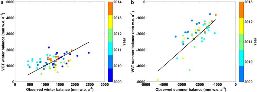
918                           Drolon and others: Monitoring of seasonal glacier MB over the European Alps using low-resolution optical satellite images

              Fig. 4. Regression results for the 55 glaciers in terms of R2, RMSE and seasonal MB. (a) RMSE (black curve) and R2 (red curve) over the winter
              calibration period 1999–2008, for the 55 studied glaciers ranked by increasing RMSE. Time series of observed winter MB (b) and winter MB
              estimated with VGT (c) over 1999–2008. For (b) and (c), each horizontal row of coloured rectangles represents the MB time series of a glacier
              (the rectangle colour indicating the MB value). Lower panels (d)–(f): respective summer equivalents of graphs (a)–(c), over 1998–2008, for the
              55 glaciers ranked by increasing RMSE. The glaciers ranking is not the same for the two seasons (winter and summer glacier ranking in
              Table S1).

Downloaded from https://www.cambridge.org/core. 16 Oct 2021 at 21:08:15, subject to the Cambridge Core terms of use.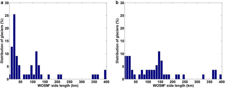
Drolon and others: Monitoring of seasonal glacier MB over the European Alps using low-resolution optical satellite images                             919

          is smaller (158 mm w.e. a−1) than the range of annual errors                             a ‘flat’ winter observed MB time series, with low interannual
          acknowledged for the glaciological MB measurements                                       variability.
          (Eobs = ±200–400 mm w.e. a−1). RMSEw_cal ranges between                                      According to Figures 4e, f, Bs_VGT time series are in agree-
          50 mm w.e. a−1 (for Gorner, #1) and 260 mm w.e. a−1 (for                                 ment with Bs_obs time series over 1998–2008. As in winter,
          Ciardoney, #55), with third quartile and median values of                                the mean differences between Bs_obs and Bs_VGT are the
          189 and 159 mm w.e. a−1, respectively. Even the highest                                  highest for 2 a with extreme summer MBs: 2003 (with strong-
          RMSEw_cal are in the same range as the lower limit for Eobs.                             ly negative MB values) and 2007 (a year with above average
          Glaciers less well-ranked in terms of RMSEw_cal (Ciardoney,                              MB). The very negative and atypical summer MB time series
          Aletsch, Cantun, respectively #55, #54, #53) are not necessar-                           of Sarennes (#23) is well estimated with SPOT/VGT (R2s of
          ily the least well-ranked in terms of R2w. Cantun for example                            0.88 and RMSEs_cal of 282 mm w.e. a−1).
          presents a relatively high RMSEw_cal (237 mm w.e. a−1) but                                   By comparing Figures 6c, d (blue dots), we observe that
          also a high R2w of 0.89 because average winter MBs are                                   the regression coefficient α values of all glaciers are much
          higher for this glacier. Thus, the two metrics (R2 and RMSE)                             more scattered in summer than in winter. In winter, αw
          are not redundant for characterizing the linear relationships                            ranges between −2.7 and −0.6 mm w.e. a−1 m−1, whereas
          between Z and observed MB for all the glaciers.                                          αs ranges between −15 and −1 mm w.e. a−1 m−1 in
              As shown in Figure 4d, the correlation between Zs and                                summer. For both seasons, we observe that the lower the ab-
          Bs_obs is also high in summer but not as much as in winter:                              solute α value, the lower the RMSE over the calibration
          the mean R2s for the 55 glaciers is 0.74, and the difference                             period.
          is also significant for the first quartile and median values (re-
          spectively 0.70 and 0.77 in summer instead of 0.79 and 0.89
          in winter). R2s is between 0.52 (Clariden, #55) and 0.88                                 4.1.2. Performance for the average of all observed
          (Sarennes, #23). The difference between the minimum and                                  glaciers
          maximum of R2s (0.36) is inferior to the same value in                                   The mean MB time series averaged for all glaciers is also
          winter (0.66), indicating a lower spread of the correlation                              interesting to study as it illustrates glacier behaviour at the
          for summer. The mean RMSEs_cal of the estimated Bs_VGT                                   scale of the entire European Alps.
          for the 55 glaciers (314 mm w.e. a−1) is twice as large as in                               In winter (Fig. 5a), ⟨Bw_VGT⟩ globally fits well with
          winter (158 mm w.e. a−1) but still acceptable compared                                   ⟨Bw_obs⟩. Absolute mean MB errors |MBEw_cal| (i.e. the
          with the error range of glaciological MB measurements.                                   mean difference between Bw_VGT and Bw_obs for all the gla-
          RMSEs_cal ranges between 134 and 528 mm w.e. a−1 (with                                   ciers) are maximal in 2005 (175 mm w.e. a−1), 2001 (110
          third quartile and median values of respectively 355 and                                 mm w.e. a−1), and to a lesser extent, in 2007 (95 mm w.e.
          299 mm w.e. a−1). Glaciers from source 2 (Table 1) present                               a−1) (Table 2). Nevertheless, these errors are small compared
          higher mean RMSEs_cal and lower R2s (391 mm w.e. a−1                                     with the standard deviation of the observed winter MB of all
          and 0.70 respectively) than glaciers from source 1 (325 mm                               glaciers σw_obs computed for 2001, 2005 and 2007, respect-
          w.e. a−1 and 0.77 respectively) and source 3 (300 mm                                     ively equal to 615, 373 and 272 mm w.e. a−1.We also note
          w.e. a−1 and 0.74 respectively). The summer RMSEs_cal                                    that the two contrasting winter balance years in 2000 and
          range (394 mm w.e. a−1) is larger than in winter (232 mm                                 2001 are well captured by the model. In summer (Fig. 5b),
          w.e. a−1) indicating a wider spread in RMSEs_cal during this                             ⟨Bs_VGT⟩ fits less well with ⟨Bs_obs⟩ than in winter although
          season. Moreover, we observe that glaciers with a poor per-                              the largest interannual variations are captured. In 2003, we
          formance in summer do not necessarily present the same                                   observe the lowest MB values reflecting the exceptional
          poor performance in winter (Table S1).                                                   summer heat wave of 2003. Absolute mean MB errors |
              Figure 4b, c show Bw_obs and Bw_VGT time series estimated                            MBEs_cal| are the highest for 2007 (448 mm w.e. a−1) and
          with SPOT/VGT, over the calibration period 1999–2008, for                                2003 (356 mm w.e. a−1). These summer errors are higher
          winter and for the 55 glaciers. By comparing Figure 4b                                   than winter errors but still inferior to σs_obs of 2007 and
          with c, it is seen that for all glaciers the Bw_obs and Bw_VGT                           2003 (respectively 594 and 559 mm w.e. a−1) (Table 2).
          time series are similar, illustrating that the ‘optimized’ rela-                         Larger errors in summer can be partly explained by higher
          tionships computed from SPOT/VGT allow a good estimation                                 interannual variability in summer observed MBs. If we con-
          of the interannual variations in winter MB over 1999–2008.                               sider the annual MB (sum of winter and summer MB;
          We note that Aletsch (the biggest glacier in the European                                Fig. 5c), the largest errors occur for 2007 and 2003 (respect-
          Alps), ranked 54th in winter (and with the lowest R2), presents                          ively 582 and 411 mm w.e. a−1), as in summer.

          Table 1. Summary of the linear regression results over the calibration period 1998/1999–2008 according to individual data sources and aver-
          aged for the 55 glaciers

                                                                  Source 1 (7 glaciers)           Source 2 (7 glaciers)    Source 3 (41 glaciers)   All glaciers (55)

          Winter            R2w_cal                               0.76                            0.72                     0.88                     0.84
                            RMSEw_cal (mm w.e. a−1)               160                             141                      160                      158
                            αw (mm w.e. a−1 m−1)                  −1.16                           −0.92                    −1.56                    −1.56
                            βw (mm w.e. a−1)                      3626                            3293                     4231                     4308
          Summer            R2s_cal                               0.77                            0.70                     0.74                     0.74
                            RMSEs_cal (mm w.e. a−1)               325                             391                      300                      314
                            αs (mm w.e. a−1 m−1)                  −4.39                           −6.69                    −5.16                    −5.25
                            βs (mm w.e. a−1)                      11 579                          19 785                   14 573                   14 722

Downloaded from https://www.cambridge.org/core. 16 Oct 2021 at 21:08:15, subject to the Cambridge Core terms of use.
920 Drolon and others: Monitoring of seasonal glacier MB over the European Alps using low-resolution optical satellite images
4.2. Cross-validation over the calibration period
1998/1999–2008
Cross-validation results for the 55 optimized relations initial-
ly calibrated over 1998/1999–2008 indicate no negative skill
score SS, except for Seewjinen in summer (SSs = −0.08;
Fig. 6b). This is consistent with the low R2s and high
RMSEs_cal calculated for this glacier over the calibration
period (Table S1). For most glaciers, the optimized individual
relationships thus have skills to estimate the seasonal MB
over a simple average of the observed MB. In winter, SS
values are higher (⟨SSw⟩ = 0.76) than in summer (⟨SSs⟩ =
0.55) (Table 3, Figs 6a, b). In winter, glaciers from Source 3
perform better in terms of ⟨SSw⟩ and ⟨R2w_cross⟩ than others.
This is consistent with their best performance for the calibra-
tion (⟨R2w_cal⟩ = 0.88, Table 1). RMSEw_cross are slightly higher
than RMSEw_cal (Fig. 6a), but they remain satisfactory with
regard to Eref. In summer, RMSEs_cross are superior to
RMSEs_cal (Fig. 6b) and also on average slightly superior to
Eref (⟨RMSEs_cross⟩ = 440 mm w.e. a−1; Table 3). Moreover,
for both seasons, the higher the SS, the lower the RMSE
and the lower the difference between the two RMSEs
(derived from both calibration and test-cross) (Figs 6a, b).
Only Aletsch Glacier in winter and Cengal Glacier in
summer present satisfactory RMSEs (as regards to Eref) and
low SS. Therefore, for these two glaciers, despite their
RMSE, their calibrated relationships present no particular
skill over a simple average of their observed MBs.
In winter, we observe high consistency between
αw_cross_best (mean of the N αw_cross) and the calibrated αw
(Fig. 6c). Moreover, the standard deviations σ(αw_cross) in
winter are low and close to an order of magnitude smaller
than for αw_cross_best (Fig. 6e; Table 3); the same applies for
σ(βw_cross). These results allow us to conclude that the cali-
brated relationships are robust and temporally stable in
winter (except for Aletsch), despite the shortness of the time
series used for the linear regression. The outcomes show
the potential skill of the individual relations to accurately es-
timate the winter MB outside the calibration period. In
summer, the consistency between αs_cross_best and αs is also
quite high, as in winter (Fig. 6d). Nevertheless, unlike in
winter, the standard deviations σ(αs_cross) in summer are
high, especially for glaciers with high RMSEs_cal (superior to
350–400 mm w.e. a−1) (Fig. 6f; Table 3). Therefore, in
summer, we can conclude on the robustness and the
temporal stability of about 60% of the 55 calibrated relation-
ships (presenting an RMSEs_cal < 400 mm w.e. a−1 and a skill
Fig. 5. Time series of mean observed MB (red) over the calibration
score >0.65). In order to test the robustness of our approach
period and of mean VGT MB (blue) over the period covered by
outside the calibration period 1998–2008, we then compare
SPOT/VGT, averaged for the 55 glaciers. The dashed red curves
represent the time series of observed MB±the standard deviation
seasonal VGT MB time series and independent observed MB
for all glaciers. (a) Winter MB for the calibration period, 1999– data (not used for calibration) over the evaluation period
2008 and the period covered by SPOT/VGT, 1999–2014. (b) 2009–2014.
Summer MB for the calibration period, 1998–2008 and the period
covered by SPOT/VGT, 1998–2013. (c) Annual MB (sum of winter
and summer MBs) over 1999–2013.
4.3. Performance over the evaluation period 2009–
2013/2014
The agreement between VGT MB estimations and The winter and summer MB averaged for all 55 glaciers esti-
observed MB over the calibration period presented above mated with SPOT/VGT (in blue) after 2008 are shown in
is satisfying. In order to test the robustness of our approach, Figure 5. In winter (Fig. 5a), ⟨Bw_VGT⟩ values are generally
we first perform a cross-validation of the 55 regressions to above average over 2009–2014, except for 2012, where
assess the temporal robustness and skills of the regression we note a strong decrease in ⟨Bw_VGT⟩. In summer (Fig. 5b),
coefficients. We then compare seasonal VGT MB time ⟨Bs_VGT⟩ is close to the average of 1998–2008, except for a
series and independent observed MB data (not used for cali- notably negative MB during summer 2012. Table S2
bration) over the evaluation period 2009–2014. (Supplementary Material) presents for each glacier, estimates
Downloaded from https://www.cambridge.org/core. 16 Oct 2021 at 21:08:15, subject to the Cambridge Core terms of use.Drolon and others: Monitoring of seasonal glacier MB over the European Alps using low-resolution optical satellite images 921
Table 2. Mean mass balance error MBE averaged for all glaciers and standard deviation σ of the observed MBs, per year and for the overall
calibration period 1998/1999–2008
98 99 00 01 02 03 04 05 06 07 08 98/99-08
Winter |MBEw_cal| (mm w.e. a−1) 58 39 110 12 15 28 175 17 99 22 58
σw_obs (mm w.e. a−1) 429 370 615 319 391 353 373 252 272 334 406
Summer |MBEs_cal| (mm w.e. a−1) 59 41 78 190 128 356 222 213 41 448 22 164
σs_obs (mm w.e. a−1) 493 460 443 301 455 559 473 494 583 594 498 596
Annual |MBEa_cal| (mm w.e. a−1) 8 103 64 146 411 257 383 38 582 31 202
σa_obs (mm w.e. a−1) 482 316 611 405 613 481 518 468 564 368 483
Fig. 6. Results of the cross-validation for all glaciers. Skill score as a function of RMSE computed for the calibration (blue) and for the test cross
(red), in (a) winter and (b) summer. Alpha derived from the calibration (blue) and from the cross-validation (red) as a function of RMSE
computed for the calibration, in (c) winter and (d) summer. Standard deviation of the alpha derived from the test-cross as a function of
RMSE computed for the calibration, in (e) winter and (f) summer.
Downloaded from https://www.cambridge.org/core. 16 Oct 2021 at 21:08:15, subject to the Cambridge Core terms of use.922 Drolon and others: Monitoring of seasonal glacier MB over the European Alps using low-resolution optical satellite images
Table 3. Summary of the cross-validation results over the calibration period 1998/1999–2008 according to individual data sources and for
the 55 glaciers
Source 1 (7 glaciers) Source 2 (7 glaciers) Source 3 (41 glaciers) All glaciers (55)
Winter SSw 0.55 0.59 0.79 0.76
R2w_cross 0.73 0.72 0.84 0.82
RMSEw_cross (mm w.e. a−1) 240 190 219 222
αw _cross_best (mm w.e. a−1 m−1) −1.12 −0.92 −1.6 −1.5
σ(αw _cross_best) (mm w.e. a−1 m−1) 0.25 0.16 0.24 0.24
βw _cross (mm w.e. a−1) 3516 3287 4334 4230
σ(βw _cross) (mm w.e. a−1) 546 396 514 518
Summer SSs 0.59 0.59 0.55 0.55
R2s_cross 0.71 0.67 0.74 0.71
RMSEs_cross (mm w.e. a−1) 437 504 457 440
αs _cross_best (mm w.e. a−1 m−1) −5.19 −6.62 −4.30 −5.08
σ(αs _cross) (mm w.e. a−1 m−1) 1.22 1.44 0.99 1.19
βs_cross_best (mm w.e. a−1) 14 612 19 570 11 284 14 188
σ(βs _cross) (mm w.e. a−1) 3874 4743 3145 3781
of both winter and summer MB over 2009–2014 and 2009– calibration period (Table S1). 2011 and 2013 are the most
2013 respectively. In order to evaluate these VGT MB calcu- poorly estimated years (RMSEw_eval of 587 and 501 mm
lations (over 2009–2014 for winter and 2009–2013 for w.e.), whereas 2010 and 2014 are best represented
summer), we now compare them with observed MBs avail- (RMSEw_eval of 252 and 245 mm w.e.; Table 4). RMSEw_eval
able for a subset of the 55 glaciers used for the calibration calculated from all data in the evaluation period (n = 66) is
(19 glaciers in winter and 13 in summer). 411 mm w.e. a−1 and thus nearly three times larger than
For winter, 70% of the computed MB present an error the average RMSEw_cal (150 mm w.e. a−1) computed for the
smaller than the estimated uncertainty in the direct mea- same subset of 19 glaciers over the calibration period.
surements Eobs max (Fig. 7a). We find the highest errors However, RMSEw_eval is still comparable with Eobs max
MBEw_eval for Sarennes and Ciardoney (−1015 mm w.e. in and the mean MB error MBEw_eval is close to zero (16 mm
2009 and −850 mm w.e. in 2011). This result is not surpris- w.e. a−1), suggesting that Bw_VGT estimations are unbiased.
ing as these glaciers are subject to a high RMSEw_cal over the To sum it up, our approach is able to estimate the winter
Fig. 7. Seasonal mass balances estimated with SPOT/VGT as a function of observed (a) winter and (b) summer MBs for glaciers over
the evaluation period 2009–2014. The 1:1 agreement is plotted (bold line). The uncertainty in each MB measurement Eobs max (±400 mm
w.e. a−1) is not represented for the sake of clarity.
Table 4. MB error MBE and RMSE per year and for the overall evaluation period 2009–2013/2014
2009 2010 2011 2012 2013 2014 2009–2013/14
Winter Number of observed MB available 13 13 11 9 6 14 66
MBEw_eval (mm w.e. a−1) −111 95 546 −326 −362 25 16
RMSEw_eval (mm w.e. a−1) 460 252 587 394 502 245 411
Summer Number of observed MB available 12 13 10 8 6 49
MBEs_eval (mm w.e. a−1) 664 −132 23 78 140 162
RMSEs_eval (mm w.e. a−1) 756 432 660 424 230 561
Downloaded from https://www.cambridge.org/core. 16 Oct 2021 at 21:08:15, subject to the Cambridge Core terms of use.Drolon and others: Monitoring of seasonal glacier MB over the European Alps using low-resolution optical satellite images 923
MB out of the calibration period for glaciers in the Alps with hypothesis, we estimate for each season, the mean number
an acceptable mean overall error and without bias. of pixels Np with a NDSI higher than 0.2 in each optimized
In summer, 60% of the computed MB present an error in- WOSM sizes centred on Clariden Glacier. This glacier was
ferior or equal to Eobs max (Fig. 7b). Largest errors MBEs_eval chosen for its much lower performance in summer (R2s =
are about two (to three) times superior to Eobs max (e.g. 0.52; RMSEs_cal = 528 mm w.e. a−1) than in winter (R2w =
Gietro with an error of 1695 mm w.e. a−1 in 2011) 0.92; RMSEw_cal = 130 mm w.e. a−1). At Clariden, the opti-
(Table 4). 2009 and 2011 are poorly estimated (resp. mized WOSM for winter (29 km × 29 km), gives a value of
RMSEs_eval of 756 and 660 mm w.e.), but summer 2013 is Np that is ∼6 times higher in winter (840) than in summer
correctly reproduced (low RMSEs_eval of 230 mm w.e.). (144). With the optimized summer WOSM (225 km × 225
RMSEs_eval calculated for the 49 evaluation points (561 mm km), Np is ∼12 times higher for winter (19 971) than for
w.e. a−1) is ∼1.5 times larger than the RMSE calculated summer (1541). Thus, Np increases with WOSM size for
over the calibration period for the subset of 13 glaciers both seasons.
used for evaluation (RMSEs_cal = 368 mm w.e. a−1). This justifies the enlargement of the optimized WOSM* in
RMSEs_eval is also higher than winter RMSEw_eval and than summer in order to integrate more snow cover variability
Eobs max. The mean MBEs_eval for the 49 points is not (Fig. 8). The distribution of WOSM* sizes is more spread
negligible (162 mm w.e. a−1), which indicates that Bs_VGT towards larger windows: the median WOSM* side length is
estimations are slightly positively biased during 2009– 119 km in summer against 43 km in winter. The need to in-
2013. This positive bias is mainly due to a strong bias (664 crease the window size in summer suggests relatively homo-
mm w.e. a−1) during summer 2009. No obvious explanation geneous snow variations in summer across the Alps. This
was found for this anomalous year. Excluding summer 2009, result is in agreement with the homogeneous summer abla-
the MBEs_eval is reduced to 52 mm w.e. a−1. However, valid- tion observed on glaciers across the entire Alpine Arc
ation is made with fewer points in summer than in winter. (Vincent and others, 2004). Pelto and Brown (2012) also
Furthermore, glaciers used for evaluation in summer are noted a similarity of summer ablation across glaciers in the
not the best performers over the calibration period: North Cascades.
the mean RMSEs_cal of the 13 evaluation glaciers (368 mm Another reason for the difference in results between the
w.e. a−1) is higher than the mean RMSEs_cal of the entire seasons might be the cloud interpolation. For each season,
(55 glaciers) dataset (318 mm w.e. a−1). we calculate the percentage of interpolated pixels for glaciers
Observed MB measurements for more glaciers and more with low RMSE (inferior to the first quartile value) and high
years will be welcome to improve the robustness of the RMSE (superior to the third quartile), averaged over the cali-
linear regressions between MB and Z in summer and to bration period. In winter, the mean percentage of interpo-
provide a more representative error RMSEs_eval on the MB lated pixels is large (4%) and the difference between high
estimated with SPOT/VGT. and low RMSE glaciers is small: the mean difference over
the 1999–2014 period is 0.13%. In summer, a striking differ-
ence is observed between glaciers with high and low RMSE:
5. DISCUSSION AND PERSPECTIVES the mean difference of the interpolated pixels percentages
(0.64%) is more than four times larger than in winter.
5.1. Method performance Therefore, the temporal interpolation seems to have more
Our method performs better in winter than in summer impact in summer than in winter. Our hypothesis to
because it is based on the interannual dynamics of the alti- explain this observation is that the cloud mask performs
tudinal snow cover distribution to retrieve the interannual less well for some glaciers in summer, but this needs to be
variation of seasonal MBs. In summer, the interannual dy- further explored.
namics are more difficult to capture as there is less snow. The effect of pixels contaminated by undetected clouds
The lower number of snow-covered pixels in summer than can also be another reason explaining the reduced perform-
in winter constitutes in fact a limit to retrieve smooth ance for summer. The spectral signatures in the available
curves of altitudinal NDSI distribution. To justify this bands of clouds and snow are close, indicating that cloudy
Fig. 8. Distribution of glaciers (%) as a function of their WOSM* side length (a) in winter and (b) in summer.
Downloaded from https://www.cambridge.org/core. 16 Oct 2021 at 21:08:15, subject to the Cambridge Core terms of use.You can also read