Estimates of abundance and distribution of cetaceans in the Black Sea from 2019 surveys
←
→
Page content transcription
If your browser does not render page correctly, please read the page content below
Estimates of abundance and
 distribution of cetaceans in the
 Black Sea from 2019 surveys

 ©CeNoBS

 ©CeNoBS

©CeNoBS ©Clean Seas

 With financial
 support of the
 European Union
Authors:
Romulus-Marian Paiu, Simone Panigada, Ana Cañadas, Pavel Gol’din, Dimitar Popov, Léa David, Ayaka
Amaha Ozturk, Dmitri Glazov

Contributors:
Svetlana Artemieva, Galina Balusheva, Laura Boicenco, Ayhan Dede, Erdem Danyer, Ertug Duzgunes,
Zurab Gurielidze, Phil Hammond, Natia Kopaliani, Irina Makarenko, Galina Meshkova, Otilia Mihail,
Mihaela Mirea-Candea, Evgeny Nazarenko, Bayram Öztürk, Angelica Paiu, Marina Panayotova, Gleb
Pilipenko, Vincent Ridoux, Miroslava Robinson, Olga Shpak, Costin Timofte, Arda M. Tonay, Karina
Vishnyakova

ASI/CeNoBS Aerial surveys Team leaders and Observers: Romulus-Marian Paiu, Dimitar Popov and Ayhan
Dede, Pavel Gol’din, Galina Meshkova, Costin Timofte, Arda M. Tonay

ASI/EMBLAS-Plus Russian Black Sea Survey Team Leader and Observers: Dmitri Glazov and Svetlana
Artemieva, Evgeny Nazarenko, Gleb Pilipenko, Olga Shpak

ASI/CeNoBS survey coordination and administrative support:
ASI Scientific Coordinator: Simone Panigada

CeNoBS Scientific Coordination working group: Ana Canadas, Lea David, Pavel Gol’din, Romulus-Marian
Paiu, Simone Panigada, Dimitar Popov, Marine Roul

CeNoBS Lead Partner Mare Nostrum: Mihaela Candea-Mirea, Marian Paiu

ACCOBAMS Secretariat: Julie Belmont, Florence Descroix-Comanducci, Célia Le Ravallec, Susana Salvador

Special thanks to the National Authorities, to the CeNoBS Advisory board members, to the aerial companies
Action Air Environment and AeroVolga and its pilots, and to the ACCOBAMS Scientific Committee for its
ambition and continuous support to the development of the ASI project since the ACCOBAMS origin.

ASI/CeNoBS survey Technical Partners:

The ASI/CeNoBS Survey was funded by ACCOBAMS and the European Union.
ASI/EMBLAS-Plus Survey Technical partners:

The ASI/EMBLAS-Plus Russian Black Sea Survey was funded thanks to ACCOBAMS and the international
Project «Improving Environmental Monitoring in the Black Sea — Selected Measures» (EMBLAS-Plus).

Citation:
ACCOBAMS, 2021. Estimates of abundance and distribution of cetaceans in the Black Sea from 2019
surveys. By Paiu, R.M., Panigada, S., Cañadas, A., Gol’din, P., Popov, D., David, L., Amaha Ozturk, A., Glazov,
D. Ed. ACCOBAMS - ACCOBAMS Survey Initiative/CeNoBS Projects, Monaco, 54 pages.

Disclaimer:
The designations employed and the presentation of the information on this document do not imply the
expression of any opinion whatsoever on the part of ACCOBAMS concerning the legal status of any
country, territory, city or area or of its authorities, or concerning the delimitation of its frontiers or
boundaries. The views expressed in this report are those of the author(s) and do not necessarily reflect
the views or policies of ACCOBAMS and European Union. The European Commission is not responsible for
any use that may be made of the information it contains.
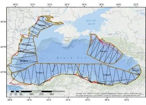
Table of Contents

FOREWORD................................................................................................................................................... 4

I. INTRODUCTION ......................................................................................................................................... 5

II. METHODS ................................................................................................................................................. 7
 II.1 Aerial survey ....................................................................................................................................... 7
 II.2 Survey design ...................................................................................................................................... 9
 II.3 Data analysis ..................................................................................................................................... 11
 II.3.1 Design-based analysis................................................................................................................ 11
 II.3.2 Model-based analysis ................................................................................................................ 14

III. RESULTS ................................................................................................................................................. 19
 III.1. Sightings.......................................................................................................................................... 19
 III.2. Abundance and Density estimation ............................................................................................... 27
 III.2.1. Design-based analysis.............................................................................................................. 27
 III.2.2. Model-based analysis .............................................................................................................. 34
 III.3. Modelling results ............................................................................................................................ 36
 III.3.1. Predictive maps for common dolphin ...................................................................................... 36
 III.3.2. Predictive maps for bottlenose dolphin ................................................................................... 41
 III.3.3. Predictive maps for harbour porpoise ..................................................................................... 45

IV. DISCUSSION ........................................................................................................................................... 47
 IV.1 Methodological aspects .................................................................................................................. 47
 IV.2 Common dolphins ........................................................................................................................... 48
 IV.3 Bottlenose dolphins ........................................................................................................................ 49
 IV.4 Harbour porpoises........................................................................................................................... 50

V. CONCLUDING REMARKS ......................................................................................................................... 51

VI. REFERENCES .......................................................................................................................................... 52

 3
FOREWORD

The aerial surveys conducted in the Black Sea in 2019 were carried out under the umbrella of the
ACCOBAMS Survey Initiative, within the framework of the CeNoBS project “Support MSFD
implementation in the Black Sea through establishing a regional monitoring system of cetaceans (D1) and
noise monitoring (D11) for achieving GES” (https://www.cenobs.eu/) and through a collaboration with
the EMBLAS-Plus project “Improving Environmental Monitoring in the Black Sea – Selected Measures”
(http://emblasproject.org/).

CeNoBS is financially supported by the European Commission, under the DG ENV call for proposals
“Marine Strategy Framework Directive - Second Cycle: Implementation of the new GES Decision and
Programmes of Measures”, and ACCOBAMS through the ACCOBAMS Survey Initiative.

CeNoBS project tackles MSFD Descriptor 1 – Biodiversity/cetaceans and Descriptor 11 – Energy including
underwater noise in the Black Sea, improving the second cycle of MSFD implementation, by achieving
greater consistency and coherence in determining, assessing and achieving good environmental status.

The main objectives of this project are:
 • assessing D1 cetaceans related criteria and supporting the establishment of thresholds values,
 • assessing and supporting the development of D11 monitoring in the Black Sea and
 • enhancing coordination among the Black Sea region throughout the dissemination of the project
 activities, results and outcomes.

CeNoBS activities aim to fill the lack of background data on the distribution/abundance of cetacean
populations and on bycatch pressure in the Black Sea and the lack of national expertise to implement
effective noise monitoring.

The EMBLAS-Plus project is funded by the European Union and it is aimed at improving protection of the
Black Sea environment through further technical assistance focused on marine data collection and local
small-scale actions targeted at reduction of pollution by marine litter, public awareness raising and
education.

Within the framework of the EMBLAS-Plus project, a collaboration was established between ACCOBAMS
and Russian scientists from the A.N. Severtsov Institute of Ecology and Evolution, Russian Academy of
Sciences, and the Federal State Budgetary Institution N.N. Zubov’s State Oceanographic Institute to
extend the coverage of the aerial survey to Black Sea Russian waters, from the Adler district of Sochi to
the midline of the Kerch Strait (Krasnodar Krai).

This report provides the results of the analysis conducted with the cetacean related datasets collected
during both CeNoBS and EMBLAS-Plus aerial surveys. It is based on CeNoBS Deliverable 2.2.2. “Detailed
Report on cetacean populations distribution and abundance in the Black Sea, including proposal for
threshold values”.

 4
I. INTRODUCTION

The Black Sea is one of the most vulnerable regional seas. Three species of odontocetes, Black Sea
common bottlenose dolphin (Tursiops truncatus ponticus Barabash, 1940), Black Sea short-beaked
common dolphin (Delphinus delphis ponticus Barabash, 1935), and Black Sea harbour porpoise (Phocoena
phocoena relicta Abel, 1905) inhabit the basins of the Black and Azov Seas.

A comprehensive abundance estimate for the entire Black Sea has never been conducted, and the largest-
scale surveys mostly date back to 1987 and earlier. Since then, a study on bottlenose dolphins and short-
beaked common dolphins in the waters of Ukraine and Russia (along the Crimean and Caucasian coasts
to a depth of 200 m and in the Kerch Strait) was carried out in 2002-2003 (Birkun et al., 2003). Based on
the results of a vessel survey in September-October 2003 in coastal waters of Crimea and the Caucasus,
the following estimates were obtained: 1 157 ± 602 individuals of harbor porpoises, 4 193 ± 1 090
individuals of bottlenose dolphins, and 5 376 ± 1 718 individuals of common dolphins (Birkun et al., 2004).

In addition, there were local surveys, mostly in coastal waters, conducted by NGO research groups1,
research institutes2 and academia 3 (Baș et al., 2019; Birkun et al., 2004; 2006; 2014; Dede & Tonay, 2010,
Gladilina & Gol’din, 2016; Gladilina et al., 2017, Kopaliani et al., 2015; Mihalev, 2005; Paiu et al., 2019;
Panayotova & Todorova, 2015; Popov et al., 2017).

The only large-scale abundance estimation of cetaceans in the riparian country’s waters was conducted
in 2013 along the North Western Black Sea (Birkun et. al., 2014) covering Ukrainian, Romanian and
Bulgarian waters, for all the three species. Estimates were indicating an abundance of 29 465 (95%CI
19568 – 44368) individuals of harbour porpoise, 60 400 (95%CI 41 316 – 88 298) of common dolphins and
26 462 (95%CI 19586 – 35751) of bottlenose dolphins.

In 2019, in cooperation and with support from ACCOBAMS in the framework of the ACCOBAMS Survey
Initiative, two international teams worked hand by hand within two riparian projects "Support MSFD
implementation in the Black Sea through establishing a regional monitoring system of cetaceans (D1) and
noise monitoring (D11) for achieving Good Environmental Status” (CeNoBS) and "Improving
Environmental Monitoring in the Black Sea – Selected Measures" (EMBLAS-Plus) to assess the status of
the Black Sea cetaceans.

Within the CeNoBS framework, this activity was part of the CeNoBS Work Package 2, focusing on the
‘Assessment of cetacean populations distribution and abundance at the regional scale’, which has been
coordinated by ACCOBAMS and Mare Nostrum with the participation of other project Partners (Green
Balkans (Bulgaria), Turkish Marine Research Foundation - TUDAV (Turkey), Ukrainian Scientific Center of
Ecology of the Sea – UkrSCES (Ukraine), National Institute for Marine Research and Development – NIMRD
(Romania)).

1 e.g. Mare Nostrum NGO - Romania, Green Balkans NGO - Bulgaria, Turkish Marine Research Foundation - TUDAV – Turkey,
BREMA - Ukraine
2 e.g. UKRSCES, TNU - Ukraine; IO-BAS – Bulgaria, P.P. Shirshov Institute of Oceanology RAN, A.N. Severtsov Institute of Ecology

and Evolution - Russia
3 Ilia State University – Georgia, Russian Academy of Sciences – Russia, Istanbul University – Turkey

 5
Due to the constraints imposed for the moment in the area, the CeNoBS project proposes the biggest
coverage ever included in a cetacean Black Sea survey, allowing to cover half of the sea. A complementary
survey was conducted in Russian waters through the EMBLAS-Plus project, in collaboration with N.
Severtsov Institute of Ecology and Evolution, Russian Academy of Sciences, and the Federal State
Budgetary Institution N.N. Zubov’s State Oceanographic Institute, using the same methodology and
protocols to allow statistical comparison of the results and to facilitate merging the data for the analysis.

The main aim of these surveys was to assess cetacean’s density and abundance in the Black Sea, by
applying the most robust and up-to-date methodology. Shared and systematic protocols have been used,
to facilitate data comparison and to create a baseline data to allow future analysis in time and space, to
assess eventual trends. A robust analytical modelling framework was applied to the dataset, facilitating
training activities for scientists in the region and encouraging a participatory approach.

This report provides the results of the analysis conducted with the cetacean related datasets collected
during both CeNoBS and EMBLAS-Plus aerial surveys. Under the CeNoBS project, these results are used to
initiate the definition of the MSFD thresholds values for cetaceans related indicators and criteria, in
particular D1C2 (cetaceans populations abundance) and D1C4 (cetacean distributional range), in line with
the new GES Decision (Commission Decision (EU) 2017/848).

 6
II. METHODS

II.1 AERIAL SURVEY
Cetacean populations’ distribution and abundance were assessed through a regional aerial survey aimed
at collecting visual observations of cetaceans following specific and shared/standardized protocols. The
aerial survey methodology offers the possibility of a large coverage in a short period of time and is the
most precise and robust approach for estimating the abundance of some cetacean species. The Black Sea
is known for its rough sea conditions and the capacity of going from 0 (calm sea) to 5 (rough sea) sea state
in a matter of minutes. Therefore, using planes has allowed the necessary flexibility for easily adapting to
weather constraints.

The line transect distance sampling method was used for the survey. In this method data are collected by
observers on board of aircrafts following specific transects designed to ensure an equal coverage
probability and representation of the study area (Buckland, 2001, 2004; Buckland et al., 2015). This
standardized approach is used in several other regional contexts (SCANS initiative – Small Cetaceans in
the European Atlantic waters and North Sea – and more recently during the Mediterranean surveys
conducted by ACCOBAMS in 2018 within the framework of the ACCOBAMS Survey Initiative project), and
it is globally recognized as the best approach to assess distribution, density and abundance of cetacean
species at large scale. In particular, several EU-countries implement this methodology as part of their
cetaceans MSFD monitoring programmes.

The data collection protocols and the survey design were prepared by a Scientific Coordinator in close
collaboration and consultation with scientists from the CeNoBS project Partners4 and partnering Scientific
organisations from Russia5. The aerial survey has covered the waters of Romania, Bulgaria, Turkey,
Ukraine, Georgia and Russia (territorial waters and exclusive economic zones) following pre-defined
transect lines within different blocks. The survey design was adjusted according to Flight Information
Regions (FIRs) constraints, as this was limiting the possibility of flying in specific areas.

While targeting cetaceans was the highest priority during the aerial survey, other relevant observations
were made in relation with D1 (biodiversity) and human activities (marine traffic, fisheries). In relation
with the GES Descriptors, the aerial survey did also collect information on D10 Marine Litter. The aerial
survey was conducted using three small planes, 2 Cessna 337 and one La-8, equipped with 2 engines, high
wings and bubble windows, to allow the vertical view by the observers. Flights were conducted during
daytime, with good weather conditions (
All teams have worked under the supervision of the Scientific Coordinator who was in charge of the
different phases before the field work, as well as a regular monitoring of the implementation of the aerial
surveys, to ensure appropriate use of the methodology, providing guidance and advice to the Team
Leaders in their flight planning, and to validate the collected data. The Scientific coordinator was also in
charge of training the teams on the distance sampling methodology and data collection protocols.

During the surveys, target altitude was 183m (600 feet) as customarily dealt in other surveys such as
SCANS, SAMM, OBSERVE or REMMOA, and ASI, with target speed of 100 knots. The data recorder used
SAMMOA software6, dedicated to data acquisition on marine megafauna from visual observation during
aerial survey, developed by Pelagis Observatory-La Rochelle University-CNRS with technical support of a
data processing office Code Lutin. SAMMOA is connected to a GPS and has a simultaneously audio
recording system. SAMMOA allows to establish a flight plan before take-off, with planned tracklines and
observer’s position onboard. SAMMOA also allows the data validation with the same interface and the
checking, thanks to the voice recordings associated to each visual observation.

EcoOcéan Institut took part in the training of the teams for the use of SAMMOA software and
significant amount of time was spent to ensure good coding of the different kind of sightings and
homogeneity in coding for all observers. Plenary sessions were run to train, discuss and fix the different
parameters to collect within SAMMOA, with the right codes. This process enhances the coherence and
standard way to collect data and reduce a lot of mistakes, heterogeneity between observers or missing
data. The attendees went through the auto-validation process together during the training, so the data
received had a high quality. The communication through the WhatsApp group with Team Leaders during
the validation process helped in real time to solve problems with the software and data storage, and
verification of the data collected.

The survey was conducted flying along the planned surveys primarily in passive mode, unless it was
necessary to obtain reliable estimates of school size or confirm species by circling over the sighted
animals. The survey was then resumed at the exact point it was left and all the secondary sightings (i.e.,
the additional sightings made after leaving the predetermined trackline) although recorded have not been
used to obtain the abundance and density estimates. The environmental conditions, reported by the
observers, were recorded at the beginning of each transect and/or whenever a change occurred. The
variables collected are the sea state (Beaufort scale), glare, cloud cover, turbidity of the sea and overall
general sighting conditions. Sightings data, also reported by the observers, included species, group size
and composition, direction of swimming and group behavior. Other accessory information such as the
presence of human activities was also recorded. Observations were made through so-called bubble-
windows allowing direct view on the track-line below the plane and recorded on a laptop with dedicated
software (Fig. 1). The plane position, speed and altitude were continuously recorded through a GPS and
angle were measured with a clinometer.

6SAMMOA 1.1.2. Système d'Acquisition des données sur la Mégafaune Marine par Observations Aériennes, Software developed by UMS 3462
Pelagis LRUniv-CNRS and Code Lutin (2012-2019).

 8
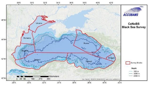
Fig. 1 – A schematic for data collection of sightings during aerial survey.

At the end of the survey EcoOcéan Institut proceeded with the pre-treatment of the data collected during
the survey (data verifying, data cleaning, and data extracting) in view of the analysis, in direct link with
Team Leaders and task coordinators. The data were sent to the specialist in charge of the analysis based
on her recommendation for the format.

II.2 SURVEY DESIGN
A total of 6 blocks were originally created (Fig. 2.). The rationale for the blocks boundaries was the best
compromise achieved between oceanographic zones, bathymetric characteristics, and
political/jurisdictional constraints. The first two are likely to have a marked effect on cetacean
distributions. The design of the blocks was constantly updated as the survey was approaching, to take into
consideration last minute issues related to permit issues and other logistical considerations, such as Flight
Information Region (FIR) boundaries regulations, as this had influence on flight authorizations.

 9
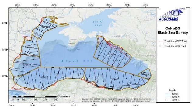
Fig. 2 – The original six blocks for the six countries of CeNoBS and the EMBLAS-Plus block, added in a second phase.

For all blocks equal spaced zigzag (ESZ) design was selected. The direction of the tracks was set to be as
perpendicular as possible to depth contours and the coast, according to best practice for distance
sampling, as in this way tracks would generally be perpendicular to the gradient of cetacean density.

The design aimed to achieve a minimum of 3% coverage of the areas, in order to be consistent with the
Mediterranean survey, conducted in summer 2018. Five hundred iterations of each design were run in
order to obtain the map of coverage probability (to assess whether it was homogeneous or not, by
calculating the probability of tracks passing over every single point of the area), and the mean percentage
coverage, mean total on effort trackline length and mean total trackline length.

The survey design was performed using the dedicated software Distance 7.3 that allows to choose the
effort for each block, the orientation of the different tracks and calculate the best route to guarantee that
each area has the same possibility of being covered by the planes (Thomas et al., 2010). This is called Equal
Coverage Probability and ensuring that the collected data are robust and statistically valid (see Buckland
et al., 2001, for further information and details on the methodology). The selected tracks allowed a final
coverage of 5% for all the areas. Figure 3. shows the tracks actually covered during the survey by the two
teams.

 10
Fig. 3 – The tracks covered by the two planes (black=on effort; red=off effort).

II.3 DATA ANALYSIS
The collected data was analyzed to estimate abundance, density and assess distribution of the different
species. Data analysis was performed with the support of skilled experts, using both model-based and
design-based frameworks.

II.3.1 Design-based analysis
Analysis of the data followed standard line transect methodology (Buckland et al., 2001). Density of
schools was estimated from the number of schools sighted, the length of transect searched and the
estimated esw (effective strip half-width: probability * truncation (strip) width). The equation that relates
density to the collected data is:
 ns
 Dˆ =
 2 esw L

where ̂ is density (the hat indicates an estimated quantity), n is the number of separate sightings of
schools, s̅ is mean school size (see below), L is the total length of transect searched, and esw is the
estimated effective strip half-width. The quantity 2 eswL is thus the area of the strip that has been
searched. The effective strip half-width is estimated from the perpendicular distance data for all the
detected animals. It is effectively the width at which the number of animals detected outside the strip
equals the number of animals missed inside the strip, assuming that everything is seen at a perpendicular
distance of zero. To calculate the effective strip half-width, we fitted a detection function (see below and
Buckland et al., 2001 for further details).

 11
Abundance was estimated as:
 Nˆ = A Dˆ
where A is the size of the survey area.

A detection function was obtained for the three species, as enough sample size has been collected to
estimate it for bottlenose dolphins, common dolphins and harbour porpoises.

The design-based analysis was performed in R, with an ad-hoc script prepared for this dataset. Segments
of tracks and sightings with sea state 4 (Douglas scale) or above were excluded from the analysis.

Covariates for the detection function

Detection functions were fitted to the perpendicular distance data to estimate the effective strip half-
width, esw. Multi-Covariate Distance Sampling methods were used to allow detection probability to be
modelled as a function of covariates additional to perpendicular distance from the transect line. These
covariates were defined in the survey design phase and are shown in Table 1.

 Table.1 - Covariates tested in the models and their ranges or factor levels

 Covariate Type Levels

 Sighting related
 School size Numerical
 Observer Categorical Observers names
 Effort related
 Seastate (Douglas factor & 0 (calm)
 scale) numerical 1 (very light)
 2 (light breeze)
 2.5 (isolated whitecaps)
 3 (gentle breeze)
 4 (moderate breeze)
 Seastate2 factor 0-1
 2-3
 4-5
 Swell factor & 0
 numerical 1m
 2m
 Turbidity factor & 0 (clear)
 numerical 1 (moderately clear)
 2 (moderately turbid)
 Sky glint factor & 0 (no glint)
 numerical 1 (glint)
 Glare severity factor & 0 (null)
 numerical 1 (slight)
 2 (moderate)
 3 (strong)
 Glare under factor & 0 (clear)
 numerical 1 (glare)
 Clouds numerical 0 to 8 from clear to totally
 Cloudy
 Clouds2 factor 0-2
 3-5

 12
6-8
 Subjective factor Subjective conditions in both
 sides (being E=excellent,
 G=good, M=moderate,
 P=poor)
 EE / EG / EM / GG / GM / GP /
 MM / MP / PP
 Subjective2 factor Subjective condensed into
 three classes
 EEG(EE / EG / GG)
 EMMG (EM / GM / MM)
 GPPM (GP / MP / PP)
 Time day factor am (6-12am)
 noon (12-2pm)
 pm (2-8pm)
 Aircraft factor Names of all aircrafts
 Team factor Names of all teams
 Effortstate factor Y (on track)
 N (off track)

Left truncation
By default, left truncation is set at 0 distance (i.e. no left truncation). But particularly for aerial surveys, it
is common practice to left truncate perpendicular distance data if the histograms of frequency of
perpendicular distances show that the area close to the line transect (distance=0) has clearly less
observations than a bit further away. This happens always when there are no bubble windows (the
observers cannot see right under the plane), and sometimes even when there are bubble windows (e.g.
the windows are narrow and observers find very uncomfortable to look directly under the plane,
observers tend to look further away and do not concentrate on the transect line, etc.).

After exploration of the data, it was clear that left truncation was necessary. The problem was more acute
for bottlenose dolphins and harbour porpoises. The distribution of perpendicular distances was explored
at fine detail, and the following left truncations were chosen: 30 m for bottlenose dolphins, 60 m for
harbour porpoises and 40 m for common dolphins.

Right truncation
It is common practice to right truncate perpendicular distance data to eliminate sightings at large
distances that have little or no influence on estimation of f(0) but adversely affect overall fit of the model.
After visual inspection of the data (histograms of perpendicular distances) different right truncation
distances were tested. A compromise between the comparison of the diagnostics of each of the different
truncation distances and the percentage of data lost in each one was used to decide on the final right
truncation. The diagnostics used were the qq-plots and the Cramer von Misses diagnostics (both of which
show how well the fitted function fits the observed data).

The final right truncation distances were: 325 m for common dolphins, 570 m for harbour porpoises and
320 m for bottlenose dolphins.
Considering both left and right truncation, the number of observations discarded for analysis were 130
(16.1%) for common dolphins, 174 (19.5%) for harbour porpoises and 18 (7.44%) for bottlenose dolphins.

 13
Model diagnostics and selection
The best functional form (Half Normal or Hazard Rate model) of the detection function and the covariates
retained by the best fitting models were selected based on model fitting diagnostics: AIC, goodness of fit
tests, Q-Q plots, and inspection of plots of fitted functions.

Q-Q plots (quantile-quantile plots) compare the distribution of two variables; if they follow the same
distribution, a plot of the quantiles of the first variable against the quantiles of the second should follow
a straight line. To compare the fit of a detection function model to the data, we used a Q-Q plot of the
fitted cumulative distribution function (cdf) against the empirical distribution function (edf).

For goodness of fit tests, we used the Cramer-von Mises (CvM) statistics (that focus on the squared
differences between cdf and edf). The smallest value of the CvM (and higher p-value) means better fit.
The smaller AIC was also preferred as it means a better compromise between fit of the model and its
complexity (number of parameters). The AIC was the main diagnostics used. If there were several
competing models (similar AIC within 2 points), then we looked at the CvM to asses which of them
produced a better fit.

II.3.2 Model-based analysis

Spatial and environmental covariates
Density surface models were produced by modelling species abundance as a function of environmental
covariates. A spatial grid was created covering the survey area to provide values of environmental
covariates for the effort segments and to predict abundance spatially. The resolution of the grid cells was
chosen as the finest consistent resolution that captures all available environmental covariates (10x10 km).
Environmental data was thus assigned to the centre of each grid cell.

Environmental variables were derived from a large number of data sources. They included variables such
as water depth (m), distance to the several depth contours (as proxies for coastal, continental shelf,
oceanic habitats, etc.), distance to canyons and seabed slope. As indices of marine hydrology and/or
biological activity/primary productivity, we included sea surface temperature, levels of chlorophyll-a and
others. For a complete list of variables used, see Table2.

 Table. 2. - Covariates tested in the spatial models.

 Covariate Description Units

 Fixed
 Lat Latitude dec. deg
 Lon Longitude dec. deg
 Aspect Orientation of the sea floor (0-359º) deg
 Depthmean Mean depth within the grid cell m
 Dist0 Distance to coast km
 Dist50 Distance to the 50m depth contour km
 Dist100 Distance to the 100m depth contour km
 Dist200 Distance to the 200m depth contour km
 Dist500 Distance to the 500m depth contour km
 Dist1000 Distance to the 1000m depth contour km
 Dist2000 Distance to the 2000m depth contour km

 14
DistCan Distance to canyons km
 DistEsc Distance to escarpments km
 DistCanEs Distance to canyons/escarpments km
 DistShelf Distance to the continental shelf km
 DistSlope Distance to the slope km
 DistAbyss Distance to the abyss (beyond the slope) km
 Slope Slope of the sea floor deg
Dynamic
 chl_mean Mean chlorophyll concentration for June-September mg/l
 chl_mean_season Mean chlorophyll concentration for the month the segment was mg/l
 surveyed
 mld_mean Mean mixed layer depth for June-September m
 mld_mean_season Mean mixed layer depth for the month the segment was surveyed m
 sbt_mean Mean sea bottom temperature for June-September deg.C
 sbt_mean_season Mean sea bottom temperature for the month the segment was deg.C
 surveyed
 ssc_mean Mean current intensity for June-September (upper 5 m) m/sec
 ssc_mean_season Mean current intensity for the month the segment was surveyed m/sec
 (upper 5 m)
 ssh_mean Mean sea surface height anomaly for June-September m
 ssh_mean_season Mean sea surface height anomaly for the month the segment was m
 surveyed
 sss_mean Mean sea surface salinity for June-September (upper 5 m) psu
 sss_mean_season Mean sea surface salinity for the month the segment was surveyed psu
 (upper 5 m)
 sst_mean Mean sea surface temperature for June-September (upper 5 m) deg.C
 sst_mean_season Mean sea surface temperature for the month the segment was deg.C
 surveyed (upper 5 m)
 chl_sd Standard deviation of chlorophyll concentration for June-September mg/l
 chl_sd_season Standard deviation of chlorophyll concentration for the month the mg/l
 segment was surveyed
 mld_sd Standard deviation of mixed layer depth for June-September m
 mld_sd_season Standard deviation of mixed layer depth for the month the segment m
 was surveyed
 sbt_sd Standard deviation of sea bottom temperature for June-September deg.C
 sbt_sd_season Standard deviation of sea bottom temperature for the month the deg.C
 segment was surveyed
 ssc_sd Standard deviation of current intensity for June-September (upper 5 m/sec
 m)
 ssc_sd_season Standard deviation of current intensity for the month the segment was m/sec
 surveyed (upper 5 m)
 ssh_sd Standard deviation of sea surface height anomaly for June-September m
 ssh_sd_season Standard deviation of sea surface height anomaly for the month the m
 segment was surveyed
 sss_sd Standard deviation of sea surface salinity for June-September (upper 5 psu
 m)
 sss_sd_season Standard deviation of sea surface salinity for the month the segment psu
 was surveyed (upper 5 m)
 sst_sd Standard deviation of sea surface temperature for June-September deg.C
 (upper 5 m)
 sst_sd_season Standard deviation of sea surface temperature for the month the deg.C
 segment was surveyed (upper 5 m)

 15
The dynamic covariates SST and CHL-a were obtained from SeaWiFS and MODIS-Aqua sensors and the SST of MODIS-Terra and MODIS-Aqua. Depth was extracted from ETOPO (a 1 arc-minute global relief model of Earth's surface that integrates land topography and ocean bathymetry, https://ngdc.noaa.gov/mgg/global/global.html). Its derivatives were obtained using ArcGis 10.5. Segments of effort All on-effort transects (i.e. where searching conditions were acceptable) were divided into segments (mean= 10.1 km) with homogeneous effort types, and under the assumption that little variability in physical and environmental features occurred, as they were clipped to fit each in a grid cell. Therefore, each segment was associated with the values of the covariates of the specific cell in which it fell. The clipping of the segments was done in ArcGis 10.5 using the Tool “Identity” to clip the effort lines with the grid cells, resulting in a final mean segment length of 10.2 km. As for the design-based method, segments of tracks and sightings with sea state 4 were excluded from the analysis, as were sightings beyond the truncation distances for each species. Stratification All estimates were produced for each individual block as well as for the whole of the study area (sum of the blocks). A complication of the analysis was that the Russian block was surveyed about 2 months later (in September) than the rest of the blocks. When analysing the data altogether using dynamic covariates that may change between the two survey periods, a bias or a misleading result could be obtained because of the confounding effect of potential real differences in distribution between Russia (at the easternmost part of the Black Sea) and the rest of the blocks (westernmost and southern parts), and differences due to changes in the environmental conditions within the two months lag between both surveys. Therefore, there are two fundamental problems: (a) the distribution of animals could be different in the two periods and (b) the relationship between density and environmental covariates could be different in the two periods. To explore this possibility, separate analyses were done for Russia and the rest of the blocks, and another analysis pooling together all blocks including Russia. Models structure The count of groups in each segment was used as the response variable. The abundance of groups was modelled using a Generalized Additive Model (GAM) with a logarithmic link function, and a Tweedie error distribution, very close to a Poisson distribution but allowing for some over-dispersion. The general structure of the model is: ni = exp ln(ai ) + 0 + f k ( z ik ) k where ni is the number of groups in the ith segment, the offset ai is the effective search area for the ith segment (calculated as the length of the segment multiplied by twice the effective strip half-width – esw), Ѳ is the intercept, fk are smoothed functions of the explanatory covariates, and zik is the value of the kth explanatory covariate in the ith segment. The esw was obtained for each species/species group from their detection function, according to the covariates included in it. In the case of modelled group sizes, the observed group size of each sighting was taken as a response variable, no offset was used, and the distribution family was negative binomial. 16
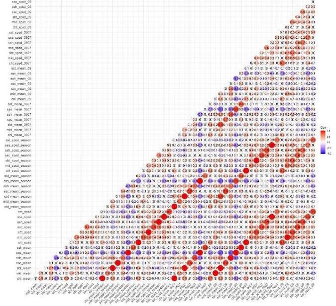
Model fitting and selection
As a first step, an exploration of correlations was performed among covariates. As a result, “families” of
covariates were created such as only one element of each family could be tested in each model. Figures
4 and 5 show the collinearity plots resulting for fixed and dynamic covariates. All correlations equal or
above 0.7 were considered as collinear and therefore not used together in the same model.

 Fig. 4 - Collinearity plot for fixed covariates

 17
Fig. 5 - Collinearity plot for dynamic covariates

REML (Restricted maximum likelihood) was used to fit the models. Shrinkage smoothers were also used
in all models, which reduces the effective degrees of freedom to zero if a covariate explains little variation
in the data.

A full model (including all covariates) was run. Using REML and shrinkage smoothers, the non-useful
covariates were discarded reducing it only to the covariates to be tested in the final models.

All the final models were run using all the potential combinations of the “useful” covariates selected by
REML and the shrinkage smoothers from the full model, sequentially testing each covariate from each
collinear family. All the resulting models were judged and ranked automatically by AIC avoiding time
consuming and unreliable manual selection.

Abundance estimation
Abundance of groups in each grid cells is estimated by multiplying the predicted density of groups from
the model (modelled count of groups with the effective search area as the offset) by the surface area of
the grid cell. Abundance per species in each grid cell were obtained then multiplying the abundance of

 18
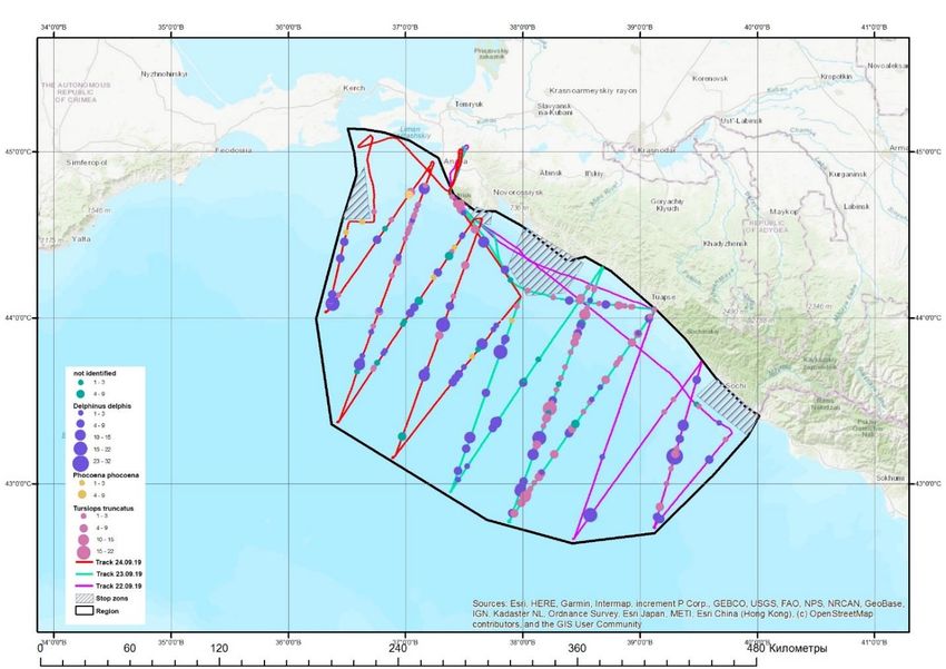
groups by the mean group size estimated for each substratum or the modelled group sizes if spatial
variation was observed.

The total abundance estimates for the whole study area and for each block were obtained by summing
up the abundance of all the grid cells comprised within the target study area.

Uncertainty
Variance of abundance was estimated by a parametric bootstrap procedure, also called “posterior
simulation”. This method generates bootstrap replicates based on resampling the parameters of the best
fitting model, instead of resampling the data itself. The delta method was used to combine the CV from
the bootstrap with the CV from the detection function and from the model. The 95% CIs will be obtained
using the final CV and assuming the estimates were lognormally distributed.
All modelling was carried out using the statistical software R (R Core Team 2017) using the mgcv package
(Wood, 2011) within an ad-hoc script created for this dataset.

III. RESULTS

Even though the plan of the CeNoBS survey was to cover all the riparian countries except Russian waters,
thanks to the cooperation with the EMBLA-Plus project a 7th block was covering partially the Russian
waters and was defined as EMBLAS-Plus. The aerial survey of the 6 blocks under CeNoBS project were
conducted between June 17th and July 4th, 2019. Two planes were employed during the survey, one
starting from Romania, in the North-West portion of the Black Sea and a second one surveying Turkish
and Georgian waters, from east to west. The Russian block was covered with a third plane, between
September 22nd and September 24th, 2019.

Given the relatively short period of time between the two surveys, and the expert’s knowledge that Black
Sea cetaceans do not extensively migrate in this time-frame, it is considered adequate to pull the data
together. Nevertheless, they were analyzed together, as well as separated, as mentioned above, taking in
consideration of actual differences.

III.1. SIGHTINGS
A total of 1,984 cetacean sightings were recorded during the aerial surveys, with 4,688 individuals from 3
different species (Table 3). A total of 15,246 kilometers was surveyed by the three planes in the different
blocks, with 9,354 km on effort and 5,892 km off effort. A summary is presented in Table 4. The aerial
survey in the waters of the Russian Federation in September 2019 included 2,030 km of effort, 15
transects. A total of 240 sightings of cetacean groups were recorded, including 94 sightings of common
dolphins, 122 sightings of bottlenose dolphins and 6 sightings of harbour porpoises.

 19
Table. 3 – The total number of sightings (left) and individuals (right) observed during the aerial surveys.

 Species Number of sightings Number of individuals
 CeNoBS EMBLAS-Plus CeNoBS EMBLAS-Plus
 Bottlenose dolphin 117 122 335 381
 Common dolphin 715 94 1762 543
 Delphinid 28 18 50 80
 Harbour porpoise 884 6 1522 15
 Total 1744 240 3669 1019

 Table. 4 – The total number of kilometres covered per block on-effort and off-effort.

 Block Km on effort Km off effort Total Km
 Bulgaria 1115.53 159.59 1275.12
 Georgia 210.36 119.12 329.48
 Romania 816.32 548.44 1364.76
 Turkey1 2211.47 2095.2 4306.67
 Turkey2 2203.03 1405.1 3608.13
 Ukraine 767.39 735.7 1503.09
 Russia 2030.3 829.4 2859.7
 Total 9,354.40 5,892.55 15,246.95

The following figures present the geographical distribution of the different species of cetaceans observed,
together with human pressures as they were sighted and recorded by the three teams (Figs. 6-18).

 Fig. 6 – Human activities in terms of naval traffic and aquaculture farms.

 20
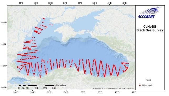
Fig. 7 – Oil pollution and fishing trash recorded by the teams.

Fig. 8 – Marine debris, including plastic debris, recorded during the surveys.

 21
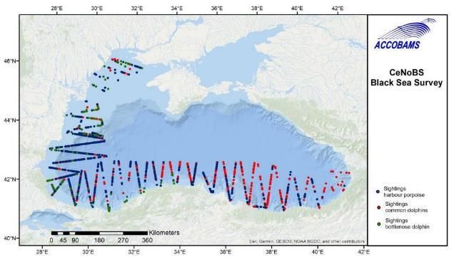
Fig. 9 – Cetaceans sightings recorded during the surveys within the CeNoBS blocks.

Fig. 10 – Cetaceans sightings recorded during the surveys within the EMBLAS-Plus block.

 22
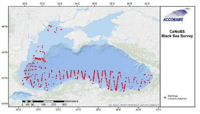
Fig. 11 – Black Sea common dolphins recorded during the surveys.

Fig. 12 – Black Sea harbour porpoises recorded during the surveys.

 23
Fig. 13 – Black Sea bottlenose dolphins recorded during the surveys.

 Fig. 14 – Marine birds recorded during the surveys.

 24
Fig. 15 – Seagull species recorded during the surveys.

Fig. 16 – Marine birds recorded during the surveys within the EMBLAS-Plus block.

 25
Fig. 17 – Human activities in terms of naval traffic recorded within the EMBLAS-Plus Block.

 Fig. 18 – Marine birds recorded during the surveys within the EMBLAS-Plus block.

 26
III.2. ABUNDANCE AND DENSITY ESTIMATION
III.2.1. Design-based analysis
The final detection functions chosen for each species and their diagnostics are presented in Table 5 and
Figures 19 to 21 The individual effect of each covariate in the selected model is presented in Figures 22 to
24.

The abundance estimates obtained with the design-based analysis for the three species of cetaceans can
be found in Tables 6 to 8. In these tables, “mean group size” is the mean of the observed group sizes,
while “expected group size” is the result of dividing the estimated abundance of individuals by the
estimated abundance of groups.

 Table 5. - Parameters and results of the detection functions. Codes: Truncation: L= left truncation (km), R= right
 truncation (km); n = number groups in detection function; key functions: HN = half-normal, HR =hazard-rate;
p=probability of detection; CV p = coefficient of variation of the probability of detection; esw = effective half-strip
 width (km); CvM p = p-value of the Cramer von Misses goodness of fit.

 Truncation
 Key
 Species L R n function Covariates p CV p esw CvM p
 seastate –
 Common
 0.04 0.325 676 HR glareunder – 0.683 0.029 0.195 0.330
 dolphins
 clouds2
 subjective2 –
 Bottlenose
 0.03 0.320 224 HR effortstate - 0.515 0.063 0.149 0.978
 dolphins
 aircraft
 seastate –
 Harbour
 0.06 0.570 717 HR turbidity – 0.318 0.029 0.162 0.949
 porpoises
 clouds2

 Q-q plot Detection function
 Fig. 19 - Q-q plot (left) and detection function (right) for common dolphins. The detection function is scaled to 1.0
at the left-truncated perpendicular distance, and the histograms represent the frequency of the observed sightings
 at different perpendicular distances. Dots represent individual sightings and the effect of the covariates
 considered.

 27
Q-q plot Detection function
 Fig. 20 - Q-q plot (left) and detection function (right) for bottlenose dolphins. The detection function is scaled to
 1.0 at the left-truncated perpendicular distance, and the histograms represent the frequency of the observed
 sightings at different perpendicular distances. Dots represent individual sightings and the effect of the covariates
 considered.

 Q-q plot Detection function
 Fig. 21 - Q-q plot (left) and detection function (right) for harbour porpoise. The detection function is scaled to 1.0
at the left-truncated perpendicular distance, and the histograms represent the frequency of the observed sightings
 at different perpendicular distances. Dots represent individual sightings and the effect of the covariates
 considered.

 28
Fig. 22- Effect of the individual covariates from the final detection function for common dolphins. The detection
function is scaled to 1.0 at the left-truncated perpendicular distance, and the histograms represent the frequency
of the observed sightings at different perpendicular distances. Dots represent individual sightings and the effect of
 the covariates considered.

 29
Fig. 23 - Effect of the individual covariates from the final detection function for bottlenose dolphins. The detection
function is scaled to 1.0 at the left-truncated perpendicular distance, and the histograms represent the frequency
of the observed sightings at different perpendicular distances. Dots represent individual sightings and the effect of
 the covariates considered.

 30
Fig. 24 - Effect of the individual covariates from the final detection function for harbour porpoise. The detection
function is scaled to 1.0 at the left-truncated perpendicular distance, and the histograms represent the frequency
of the observed sightings at different perpendicular distances. Dots represent individual sightings and the effect of
 the covariates considered.

 31
Table 6 - Results of the design-based analysis for common dolphins.

 Enc.
 CV CV
 mean exp. Rate Density
 Area n exp. Effort Enc. 95% Confidence
Stratum group group groups (Anim./ Abundance CV
 km2 groups group (km) rate Interval
 size size (per km2)
 size groups
 km)
Bulgaria 32683 72 2.43 2.49 0.1478 1187.6 0.0606 0.1445 0.4056 13258 0.2233 8568 20514
Georgia 6237 7 3.00 2.90 0.1908 329.5 0.0212 0.4260 0.2027 1264 0.4980 492 3250
Romania 18611 32 2.38 2.38 0.2796 1211.9 0.0264 0.2391 0.1413 2629 0.3564 1326 5213
Russia 48547 83 5.76 5.76 0.1018 2726.5 0.0304 0.1418 0.5215 25315 0.1962 17267 37113
Turkey1 71796 207 2.57 2.53 0.0806 3208.2 0.0645 0.1253 0.4193 30105 0.1445 22691 39941
Turkey2 69785 260 2.22 2.20 0.0767 3313.1 0.0785 0.1109 0.4222 29461 0.1451 22177 39139
Ukraine 21057 15 1.87 2.00 0.2709 1240.3 0.0121 0.3280 0.0571 1203 0.3975 564 2566
Total 268716 676 2.79 2.83 0.0533 13233 0.0511 0.0654 0.3842 103234 0.0840 87580 121687

 Table 7 - Results of the design-based analysis for bottlenose dolphins.

 Enc.
 CV CV
 mean exp. Rate Density
 Area n exp. Effort Enc. 95% Confidence
 Stratum group group groups (Anim./ Abundance CV
 km2 groups group (km) rate Interval
 size size (per km2)
 size groups
 km)
Bulgaria 32683 16 3.31 3.14 0.1971 1187.6 0.0135 0.3723 0.1387 4532 0.3809 2188 9388
Georgia 6237 0 329.5 0.0000 0.0000 0.0000 0 0.0000 0 0
Romania 18611 38 2.34 2.36 0.2340 1211.9 0.0314 0.2349 0.2090 3890 0.3709 1912 7915
Russia 48547 115 3.13 3.26 0.1114 2726.5 0.0422 0.1643 0.5124 24877 0.2306 15894 38936
Turkey1 71796 40 3.05 3.29 0.1876 3208.2 0.0125 0.2002 0.1116 8009 0.3085 4426 14494
Turkey2 69785 0 0.00 0.00 3313.1 0.0000 0.0000 0.0000 0 0.0000 0 0
Ukraine 21057 15 3.60 3.54 0.2395 1240.3 0.0121 0.2800 0.1529 3219 0.3806 1556 6656
Total 268716 224 3.03 3.17 0.0801 13233 0.0169 0.1086 0.1657 44527 0.1547 32915 60236

 32
Table 8 - Results of the design-based analysis for harbour porpoises.

 Enc.
 CV CV
 mean exp. Rate Density
 Area n exp. Effort Enc. 95% Confidence
Stratum group group groups (Anim./ Abundance CV
 km2 groups group (km) rate Interval
 size size (per km2)
 size groups
 km)
Bulgaria 32683 309 1.71 1.70 0.0694 1187.6 0.2602 0.0980 1.3855 45284 0.1351 34707 59083
Georgia 6237 0 329.5 0.0000 0.0000 0.0000 0 0.0000 0 0
Romania 18611 53 3.13 3.22 0.5900 1211.9 0.0437 0.1852 0.4498 8372 0.6238 2690 26056
Russia 48547 5 2.80 2.79 0.4157 2726.5 0.0018 0.4446 0.0182 883 0.6153 289 2697
Turkey1 71796 203 1.68 1.69 0.0777 3208.2 0.0633 0.1102 0.3178 22814 0.1300 17686 29429
Turkey2 69785 113 1.39 1.38 0.0693 3313.1 0.0341 0.1499 0.1422 9926 0.1646 7196 13690
Ukraine 21057 34 2.03 2.02 0.1533 1240.3 0.0274 0.2529 0.1753 3692 0.3376 1927 7072
Total 268716 717 1.78 1.74 0.0700 13233 0.0542 0.0740 0.3385 90970 0.0991 74902 110486

 33
III.2.2. Model-based analysis
 The parameters and selected covariates for the density surface modelling for each species are
 presented in Table 9. For harbour porpoises there were not enough sightings in the Russian block
 to run an independent model.

 Table 9. - Parameters and selected covariates. The meaning of the covariates can be consulted in Table 5; edf =
 estimated degrees of freedom; p = significance of the covariate.

 Groups Group size
 Deviance Deviance
 Species Blocks Covariates edf p explained Covariates edf p explained
 (%) (%)
 Lat,Lon 21.48 0.00000

 All Aspect 2.37 0.00188 Lat,Lon 15.63 0.00000
 except DistCanEsc 0.87 0.00496 39.82 DistCanEsc 0.85 0.00255 14.29
 Russia
 ssc_spsd_season 0.98 0.00004
 ssh_mean_season 6.12 0.00000
Common DepthMean 0.78 0.03270
 Russia DistSlope 0.89 0.00924 3.46 10.99
dolphins sst_spsd_season 0.90 0.00560
 Lat,Lon 17.04 0.00000 Lon 5.57 0.00000
 Slope 3.41 0.00023 ssc_mean_season 0.96 0.00095
 All blocks ssc_spsd 4.52 0.00000 33.72 ssc_spsd_season 5.96 0.00000 27.40
 ssh_mean 5.46 0.00000 ssh_mean_season 5.35 0.00000
 sst_spsd 0.89 0.00346

 All DistShelf 0.99 0.00004
 except Lon 0.87 0.01126 13.10 Lat,Lon 13.46 0.07404 29.62
 Russia ssh_mean_season 0.91 0.00475
Bottlenose
 Russia Lat,Lon 21.87 0.00000 45.89 DistSlope 1.98 0.00015 13.43
 dolphins
 DistCanEsc 0.89 0.00559
 DistPorts 0.98 0.00022 Dist100 0.91 0.00400
 All blocks 22.59 13.60
 ssc_spsd_season 2.58 0.00001 DistSlope 4.77 0.00018
 sst_mean 5.15 0.00000
 Lat,Lon 21.30 0.00000 Lat,Lon 13.13 0.00000
Harbour DepthMean 0.87 0.00831 Dist2000 7.57 0.00000
 All blocks 50.75 26.79
porpoise ssh_mean_season 3.13 0.00002 ssc_mean_season 8.21 0.00000

 Tables 10 to 12 show the results of abundance estimates for the model-based analysis for each species.

 34
Table 10.- Results of the model-based analysis for common dolphins for the three sets of models
 CV
 mean
 Area mean Density 95% Confidence
Dataset Stratum group Abundance CV
 km2 group (Anim./km2) Interval
 size
 size
 Bulgaria 32683 2.674 0.130 0.332 14231 0.1219 11506 18433
 Georgia 6237 2.750 0.255 0.139 1431 0.3823 735 2896
 Romania 18611 2.717 0.199 0.143 3661 0.1528 2772 4966
 Russia 48547 5.659 0.105 0.463 28657 0.1199 23732 37001
All blocks
 Turkey1 71796 2.604 0.077 0.448 38896 0.0925 33392 47553
 Turkey2 69785 2.227 0.069 0.439 38033 0.0885 33548 45686
 Ukraine 21057 1.867 0.227 0.037 1242 0.2546 806 2086
 Total 268716 2.787 0.047 0.361 118328 0.0628 109398 136922
 Bulgaria 32683 2.674 0.130 0.316 13542 0.1263 10898 17414
 Georgia 6237 2.750 0.255 0.162 1671 0.3703 882 3567
 Romania 18611 2.717 0.199 0.166 4243 0.1745 3105 6049
Without
 Turkey1 71796 2.604 0.077 0.435 37776 0.0947 32898 46341
Russia
 Turkey2 69785 2.227 0.069 0.454 39332 0.0824 34918 47264
 Ukraine 21057 1.867 0.227 0.037 1255 0.3348 747 2634
 Total 268716 2.375 0.047 0.342 90895 0.0634 84616 105659
 Russia Russia 48547 5.759 0.105 0.537 33246 0.0936 28300 40073

 Table 11. - Results of the model-based analysis for bottlenose dolphins for the three sets of models
 CV
 mean
 Area mean Density 95% Confidence
Dataset Stratum group Abundance CV
 km2 group (Anim./km2) Interval
 size
 size
 Bulgaria 32683 3.172 0.195 0.240 10262 0.2736 6094 17537
 Georgia 6237 0.110 1134 0.4190 518 2475
 Romania 18611 2.342 0.206 0.243 6208 0.2561 3968 10325
 Russia 48547 3.130 0.086 0.279 17288 0.2643 10772 28852
All blocks
 Turkey1 71796 2.957 0.134 0.198 17205 0.2849 9991 29852
 Turkey2 69785 0.229 19840 0.2862 11646 33949
 Ukraine 21057 3.600 0.250 0.131 4387 0.2890 2555 7697
 Total 268716 3.027 0.065 0.221 72369 0.2622 45174 119672
 Bulgaria 32683 3.172 0.195 0.147 6310 0.2309 4220 10282
 Georgia 6237 0.003 26 1.2699 1 209
 Romania 18611 2.342 0.206 0.149 3801 0.2249 2651 5880
Without
 Turkey1 71796 2.957 0.134 0.070 6094 0.2377 4173 9910
Russia
 Turkey2 69785 0.007 600 1.0936 74 4299
 Ukraine 21057 3.600 0.250 0.093 3101 0.2877 1881 5532
 Total 268716 2.917 0.099 0.068 18091 0.2449 14249 29922
 Russia Russia 48547 3.130 0.086 0.389 24078 0.1780 20954 39621

 35
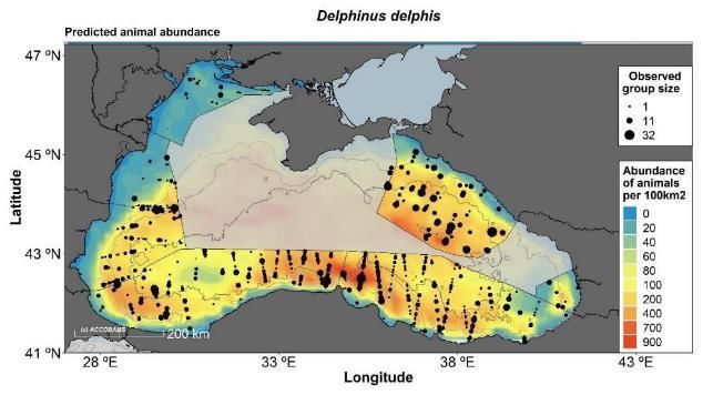
Table 12. - Results of the model-based analysis for harbour porpoise
 CV
 mean
 Area mean Density 95% Confidence
 Dataset Stratum group Abundance CV
 km2 group (Anim./km2) Interval
 size
 size
 Bulgaria 32683 1.702 0.055 1.143 48924 0.0899 42190 58986
 Georgia 6237 0.007 70 0.8996 15 347
 Romania 18611 2.391 0.450 0.426 10887 0.1384 8414 14489
 Russia 48547 1.667 0.400 0.006 380 0.5638 178 1298
 All blocks
 Turkey1 71796 1.657 0.065 0.363 31508 0.0983 27072 38719
 Turkey2 69785 1.389 0.072 0.130 11251 0.1384 8971 15152
 Ukraine 21057 2.029 0.146 0.098 3280 0.3163 2049 6324
 Total 268716 1.768 0.085 0.288 94219 0.0695 85430 109750

III.3. MODELLING RESULTS
Based on the collected data, modelling analysis were performed in order to predict the distribution and
density of the species within the different surveyed blocks. The predictive maps are presented below species
by species.

For common and bottlenose dolphins, different approaches in the data analysis have been applied and the
following maps present them in this order:
 1. Predictive maps including CeNoBS study area and Russian study area together,
 2. Predictive maps including CeNoBS study area only,
 3. Predictive maps including Russian study area only.

For harbour porpoise, only the predictive maps including CeNoBS study area and Russian study area together
are presented, as the number of observations in the Russian area was too small to perform separate models.

III.3.1. Predictive maps for common dolphin
Black Sea common dolphins were the second most common species observed during the CeNoBS aerial
surveys, with 715 sightings, totaling 1,762 individuals. This was the second most abundant species in the
Russian survey, with 94 sightings.

The following maps present common dolphin predicted density and abundance in the surveyed area (Figs.
25-33).

 36
You can also read