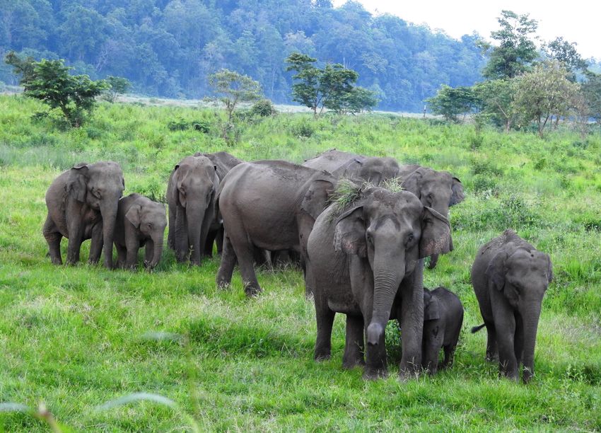
NATIONAL ELEPHANT SURVEY REPORT - STATUS OF THE MEGA-HERBIVORE IN BHUTAN - DOFPS
←
→
Page content transcription
If your browser does not render page correctly, please read the page content below
NATIONAL ELEPHANT
                                                        SURVEY REPORT
                                                        Status of the mega-herbivore in Bhutan

           Nature Conservation Division
      Department of Forests and Park Services
Ministry of Agriculture and Forests, Thimphu Bhutan
Tel: +975 02 325042/ 324131 | Fax: +975 02 335806
                   Post Box # 130
                 www.dofps.gov.bt

             ISBN-978-99936-620-8-2

 Designed and Printed by Bhutan Printing Solutions
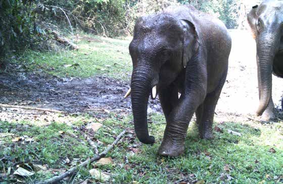
Analysis and report preparation:
Ugyen Penjor, Nature Conservation Division
Tandin, Nature Conservation Division
Sonam Wangdi, Nature Conservation Division

Data cleansing and preparation:
Phurba Lhendup, WWF Bhutan
Kuenley Tenzin, WWF Bhutan
Rinzin Dorji, Gedu Territorial Division
Ugyen Tshering, Jomotshangkha Wildlife Sanctuary
Leki Chaida, Jomotshangkha Wildlife Sanctuary
Chaten, Jomotshangkha Wildlife Sanctuary
Kinley Gyeltshen, Phibsoo Wildlife Sanctuary
Kinga Norbu, Phibsoo Wildlife Sanctuary
Tshewang Jaimo, Royal Manas National Park
Chimi Dorji, Samdrup Jongkhar Territorial Division,
Yeshi Dorji, Samtse Territorial Division,
Jigme Tenzin, Sarpang Territorial Division

Reviewers:
Dr. Varun R. Goswami, Wildlife Conservation Society, India
Dr. Raman Sukumar, Indian Institute of Science, India

Suggested citation:
NCD, 2018. National Elephant Survey Report. Nature Conservation Division,
Department of Forests and Park Services, Ministry of Agriculture and Forests,
Thimphu, Bhutan.

Photo credits: Department of Forests and Park Services, Gem Tshering and Sonam
Wangdi, Nature Conservation Division, Dorji Rabten, Phibsoo Wildlife Sanctuary

ISBN-978-99936-620-8-2
National Elephant Survey Report

                            སོ་ནམ་དང་ནགས་ཚལ་ལྷན་ཁག།
                       ROYAL GOVERNMENT OF BHUTAN
                               Ministry of Agriculture & Forests
                                 Tashichhodzong, Thimphu : Bhutan

     དྲུང་ཆེན།
    SECRETARY
                                                                                           8th August 2018

                                                  Foreword

   The elephants have long captivated the imagination of human beings. They are an integral part of
   religion and culture. In Bhutanese culture, elephants are portrayed as an important figure; the most
   prominent observed in the ‘four harmonious friends’ or Thuenpa Puenzhi. Further, the elephant also
   constitutes one of the important elements of the seven precious possessions or Rinchen Nadun. Despite
   reverence, elephants have suffered range loss and population decline due to habitat fragmentation and
   poaching. Elephants are classified as endangered by the International Union for Conservation of
   Nature (IUCN). In Bhutan, elephants are protected under Schedule I of the Forest and Nature
   Conservation Act, 1995.

   This report will be immensely helpful in developing the conservation management or action plan for
   elephants in Bhutan. The findings show that Bhutan is doing pretty fine in terms of wildlife
   conservation per se. Given the habitat and available space, a total population of more than 600
   elephants seems to be reasonable. This indicates that our conservation policies are on the right track.
   While we celebrate another milestone in our conservation journey, we also need to be cautious about
   the emerging challenges.

   I am delighted to share that, with this report, we now have national figures on most megafauna species
   (such as tiger, snow leopard, grey langur, golden langur and now elephant). With the start of the
   Twelfth Five Year Plan, it gives us an opportunity to plan and prepare for the conservation
   management of important megaherbivore and to strive to strike the balance between conservation and
   development.

   I congratulate the Department of Forests and Park Services and in particular Nature Conservation
   Division for producing this report. I also thank all field crews who were part of this survey. Lastly, my
   sincere gratitude and appreciation to the donors for supporting Bhutan in her endeavor to achieve
   conservation success.

   Trashi Delek!

   (Rinzin Dorji)

                              PHONE: +975-2-322379, FAX: +975-326834

Status of the mega-herbivore in Bhutan                                                                    i
National Elephant Survey Report

                                  དཔལ་ལྡན་འབྲུག་གཞུང་། སོ་ནམ་དང་ནགས་ཚལ་ལྷན་ཁག།
                                      ནགས་ཚལ་དང་གླིང་ཀ་ཞབས་ཏོག་ལས་ཁུངས།
                                      Royal Government of Bhutan
                                   Ministry of Agriculture and Forests
                                 Department of Forests and Park Services
                                                 Thimphu

    DIRECTOR                                                                           8th August 2018

                                                  Preface

    Elephant, the largest living terrestrial mammal is greatly revered and worshiped throughout the
    Asian culture and religion. In Bhutan, elephants are respected as godly creatures often depicted as
    wall paintings, statues and in religious ceremonies. However, the Asian elephant is listed as
    “Endangered” by the IUCN and found only in 13 range countries including Bhutan. It is indeed
    very sad that their population in the wild is declining due to habitat loss, conflict with humans and
    poaching and illegal trade. Nevertheless, Bhutan stands today as one of the most important habitats
    for this mega herbivore.

    As part of the global effort for conservation of the Asian elephants, Bhutan completed the third
    nation-wide elephant survey recently. I am very glad to introduce this National Elephant Report
    which is a testimony to Bhutan’s commitment in conserving these giant pachyderms. I am also
    pleased to state that this report is a product of latest survey methods and robust statistical data
    analyses by our own team.

    This scientific report discusses in detail about how the camera trap data along with home range
    data are being used for estimation of Asian elephant population and distribution in Bhutan. We
    estimated 678 (605-761) elephants in Bhutan at a density of 0.29 individuals/100km2 with
    estimated habitat use probability of 81% of potential elephant habitat in southern Bhutan. The
    report recommends increased habitat connectivity to reduce conflict with humans besides habitat
    improvement and increasing protection against poaching for ivory.

    I would like to express my appreciation and congratulations to the Nature Conservation Division
    for coming up with this report. I acknowledge the hard work and dedication by all the field staffs
    and others involved during the survey and data analyses. Lastly, I thank the generous financial
    support from our conservation partners particularly WWF Bhutan in this survey.

    Best Wishes and Tashi Delek!

    (Phento Tshering)

   Post Box. No. 1345 Phone: 975 (02) 323055/321185/322487, EPABX: 334458/ 334487 Fax: 322395/322836
                           Hot line: 211 website: www.dofps.gov.bt

Status of the mega-herbivore in Bhutan                                                                      ii
National Elephant Survey Report

                                 དཔལ་ལྡན་འབྲུག་གཞུང་། སོ་ནམ་དང་ནགས་ཚལ་ལྷན་ཁག།
                                     ནགས་ཚལ་དང་གླིང་ཀ་ཞབས་ཏོག་ལས་ཁུངས།
                                 Ministry of Agriculture and Forests
                                Department of Forests & Park Services
                                 NATURE CONSERVATION DIVISION

                        “Managing Bhutan’s Natural Heritage”
                                                                                           8th August 2018

                                            Acknowledgement

 The Nature Conservation Division would like to sincerely thank all the Chief Forestry Officers and survey
 team members from the elephant range protected areas and Territorial Divisions for painstakingly
 collecting the data. Without your dedication and enthusiasm, a survey of this intensity and size would not
 have been possible.

 We gratefully acknowledge the contributions of Mr. Phurba Lhendup and Mr. Kuenley Tenzin (WWF
 Bhutan), Mr. Rinzin Dorji (Gedu Territorial Division), Mr. Ugyen Tshering, Mr. Leki Chaida and Mr.
 Chaten (Jomotshangkha Wildlife Sanctuary), Mr. Kinley Gyeltshen and Mr. Kinga Norbu (Phibsoo
 Wildlife Sanctuary), Ms. Tshewang Jaimo (Royal Manas National Park), Mr. Chimi Dorji (Samdrup
 Jongkhar Forest Divisio), Mr. Yeshi Dorji (Samtse Territorial Division) and Mr. Jigme Tenzin (Sarpang
 Territorial Division) in formulation of this technical report.

 We also remain highly indebted to Dr. Raman Sukumar and Dr. Varun R. Goswami for their valuable
 feedbacks and inputs in finalizing this report.

 We would like to extend our heartfelt gratitude to the generosity extended by our partners in conserving
 and promoting our rich biodiversity. In particular, we acknowledge the generous financial support
 rendered by WWF Bhutan and Bhutan Trust Fund for Environmental Conservation in the field data
 collection and data analyses.

  Nature Conservation Division 2018

         Telephone # : +975 02 325042/324131         Fax # : +975 02 335806     Post box #: 130

Status of the mega-herbivore in Bhutan                                                                 iii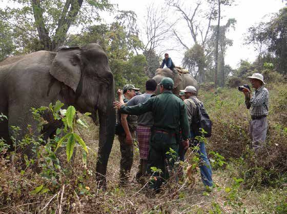
National Elephant Survey Report

Status of the mega-herbivore in Bhutan            iv
National Elephant Survey Report

Table of Contents

Executive Summary								1
1. Introduction									3
2. Materials and Methods							5
  2.1. Study area								5
  2.2. Field survey								5
  2.3. Data analysis								7
      2.3.1. Covariate preparation						7
      2.3.2. Abundance estimation						8
      2.3.3. Home range size and effective sampled area			   10
      2.3.4. Habitat use analysis						11
3. Results									13
  3.1. Detection probability and abundance					              13
  3.2. Home range size								16
  3.3. Density and population size						18
  3.4. Sex-ratio from photographic capture-recapture				     18
  3.5. Habitat use probability 							19
4. Discussion									21
  4.1. Abundance								21
  4.2. Habitat use								24
  4.3. Management implications						27
  4.4. Recommendations							28
  4.5. Study limitations							28
  4.6. Conclusion								29
5. References									31

Status of the mega-herbivore in Bhutan                            v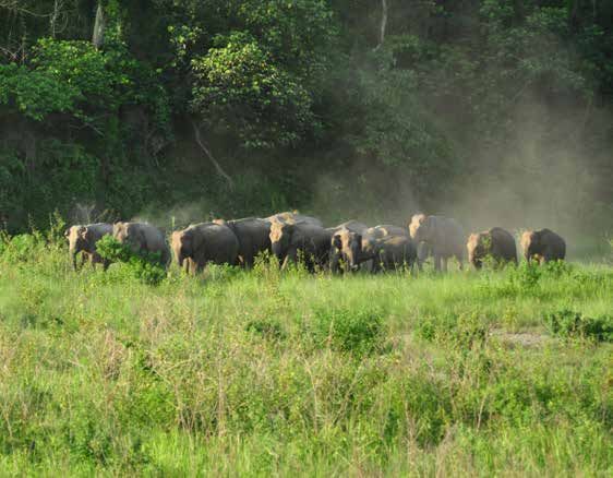
National Elephant Survey Report

List of Tables
Table 1: Pearson’s correlation matrix of continuous site covariates
Table 2: Abundance model with p(.)
Table 3: Detection models for N-mixture models
Table 4: Abundance (λ) models for N-mixture models
Table 5: Untransformed coefficients (λ; Abundance) from N-mixture models
Table 6: Untransformed coefficients (detection) from N-mixture models
Table 7: Detection models for Royle-Nichols model
Table 8: Abundance models for Royle-Nichols model
Table 9: Coefficient (untransformed) for Royle-Nichols model
Table 10: Home range estimates from the five collared elephants in Bhutan
Table 11: Detection models for occupancy models (habitat use probability)
Table 12: Occupancy models (Habitat use probability)
Table 13: Beta coefficients (untransformed) for occupancy models (Habitat use probability)

List of Figures
Figure 1. Study area and survey grids
Figure 2. Detection/non-detection matrix from elephant survey camera trap data
Figure 3. Abundance in relation to elevation and forest cover
Figure 4. Bivariate prediction of elephant abundance in Bhutan in relation to elevation and
          forest cover
Figure 5. Habitat use probability in relation to covariates (distance to river, distance to
          road, distance to settlement, slope, elevation and forest cover)
Figure 6. Predicted Asian elephant distribution in Bhutan

Status of the mega-herbivore in Bhutan                                                    vi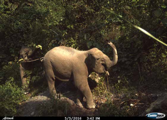
National Elephant Survey Report

Executive summary
In addition to the nation-wide surveys for tiger and snow leopard, in 2016 Nature
Conservation Division, Department of Forest and Park Services with the support of field
divisions and protected areas conducted National Elephant Survey. This survey spanned the
whole southern districts covering almost an area of 8000 km2 of potential Asian elephant
habitat in Bhutan. This survey combined multiple methods of detection using camera traps in
conjunction to dung DNA sample collection in 129 of each 25km2 grid cells. The survey was
conducted between March and June 2016. The survey aimed to estimate the elephant density
and abundance, assess the distribution and habitat use and develop a national database of the
elephant.

The analytical method for estimating elephant density and abundance involved the use
of ensemble models. The photographic records were analyzed under various modeling
frameworks such as N-mixture, Royle-Nichols, and occupancy models. The feat in the use
of these models lies in the flexibility and conspicuousness of model building. A user can
explicitly account for detection probability which is an inherent idiosyncratic problem in
ecological studies. However, there are certain model assumptions that must be adhered to
achieve reliable estimates.

The camera traps were retrieved from 123 out of 129 camera stations. The elephants were
detected at 90 out of 123 stations over the effort of 6564 trap days. For analyses, 446 images
from 123 stations were used. The elephant density is estimated at 0.29 individual per 100
km2 (95% confidence interval 0.26 – 0.33) and the total elephant numbers are estimated at
678 (range 605-761). The estimated occupancy probability is 81% (meaning 81% of the c.
8000 km2 potential elephant habitat have a high use probability by the elephants).

The adult male to female sex ratio estimated from the photographic record is 1:2.3 indicating
a stable ratio. This also implies that the current regime of intensive protection is paying
dividends. Elsewhere, the population stability is grappling with skewness due to mortality of
male (bull) elephants to poaching.

The elephant abundance and habitat use are favored by high forest cover with a mosaic
of the river system and the abundance and habitat use decrease with increased elevation.
The population is shared between Bhutan and India and conservation entails transboundary
cooperation. Further, it is recommended to perform periodic monitoring of elephant
population and demography. Furthermore, stringent anti-poaching/counter-poaching
measures should be enhanced and strengthened to ensure the safety and perpetuity of this
majestic mega-herbivore.

Status of the mega-herbivore in Bhutan                                                    1
National Elephant Survey Report

Status of the mega-herbivore in Bhutan            2
National Elephant Survey Report

1. Introduction
The Asian elephant (Elephas maximus) is feared and revered for its magnificence and sheer
power in history and culture. Elephants are portrayed as an important figure in Bhutanese
culture. The most prominent one seen in the ‘four harmonious friends’ (or Thuenpa Puenzhi)
paintings on the walls of Bhutanese structures (Jigme and Williams, 2011). Here one
can see an elephant supporting the monkey who in turn supports a rabbit and a pheasant
collaborating together to harvest the fruits of wisdom. Elephant constitutes an important
element of the seven precious possessions (or Rinchen Naduen), Langpo Rinpoche (or the
Precious Elephant) which signifies strength and power (Phuntsho, 2017). Further, elephants
are also revered as a form of Buddha (meme Sangay literally translating to ‘grandpa Buddha’
in Sharchop kha, one of the local dialects of Bhutan). Further, in Hindu culture elephants are
worshipped as Lord Ganesha (son of mighty Lord Shiva). Elephants, in addition to value as
a charismatic mega-vertebrate, is also considered as premier flagship and umbrella species
(Fernando et al., 2008). Elephants are known seed dispersers across different habitats and
potentially disperse seeds over long distances thus helping in the key process of the population
and community dynamics in plants (Corlett, 1998; Wang and Smith, 2002; Campos-Arceiz,
et al., 2008).

Status of the mega-herbivore in Bhutan                                                     3
National Elephant Survey Report

The historical range of the Asian elephant extended from west Asia through the Iranian coast
to the Indian subcontinent, eastwards into south-east Asia, including Sumatra, Java and Borneo
and Yangtze-Kiang in China, covering an area of approximately 9 million km2 (Olivier,
1978; Sukumar, 2003). Today, the range of this mega-herbivore is much reduced, and it is
considered to be under grave threat from habitat loss, degradation, conflict and ivory poaching
(Leimgruber et al., 2003; Sukumar, 2003; Goswami et al., 2007). So much so that the species
is classified as endangered under the International Union for Conservation of Nature (IUCN)
Red List of Threatened Species and listed on Appendix I of Convention on International Trade
in Endangered Species of Wild Fauna and Flora (CITES), the only living species of genus
Elephas (Sukumar, 2006).

In Bhutan, elephants are totally protected under Schedule I of the Forest and Nature Conservation
Act of Bhutan, 1995 and distributed throughout the southern belt of Bhutan (Samtse, Chhukha,
Dagana, Phibsoo Wildlife Sanctuary, Sarpang, Royal Manas National Park, Samdrupjongkhar
and Jomotshangkha Wildlife Sanctuary). They have been recorded from elevations as low as
100m to above 2000m, and have been found to use diverse habitats ranging from subtropical
forests to cool broadleaved forests.

The first nation-wide elephant survey was conducted in 2005 based on the direct observation
and block count method (Jigme and Williams, 2011). The results from this survey were
accompanied by high uncertainties because of a limited number of direct sightings. In 2010,
another survey in high elephant occurrence sites (in Samtse, Sarpang, and Phibsoo Wildlife
Sanctuary; the total studied area of 800 km2) was conducted using a more refined method: dung
transect surveys of 4-km each in grid quadrats of 25 km2 (Jigme and Williams, 2011). This
survey estimated the density of elephants to be 0.641 individuals per km2 and a total number of
513 elephants (range 30-1797; Jigme and Williams, 2011). However, this method still yielded
a very variable estimate given that the confidence interval ranged from 30 to 1797 elephants.
The most recent survey was conducted in 2016 using a much-refined survey methodology in
all sites in the southern part of Bhutan where elephant presence was previously recorded (see
details in Methodology). This method, unlike the previous methods, combined different data
collection strategies to yield better estimates of elephant abundance. The main aim of the 2016
survey was to estimate with confidence the elephant abundance in Bhutan. With discontinuous
elephant population estimates throughout the range countries, the need was felt to provide
empirical evidence to effectively manage the population that is found in Bhutan.

One of the fundamental objectives of wildlife population management, or rather any ecological
investigation, is to understand the relationship between abundance and habitat association
(Royle, 2004). The main objectives of the 2016 survey were:
    i.  Reliable estimation of Asian elephant density and abundance in Bhutan.
   ii.  Understand the distribution and habitat use of Asian elephants in Bhutan.
  iii.  Develop a national database (photographic record) of elephants.

Status of the mega-herbivore in Bhutan                                                      4
National Elephant Survey Report
2. Materials and Methods
2.1. Study area
Bhutan is a small landlocked country sharing borders with China in the north and India to
the east, west, and south. The survey was conducted in the southern region encompassing
Samtse Territorial Division, Chhukha (Gedu Territorial Division), Phibsoo Wildlife
Sanctuary, Sarpang Territorial Division, Royal Manas National Park, Samdrupjongkhar
and Pemagatshel (Samdrup Jongkhar Territorial Division) and Jomotshangkha Wildlife
Sanctuary (Figure 1).
Figure 1. Study area and survey grids
All the study sites share an international border with the Indian states of West Bengal and
Assam. The forest type throughout the study range is a mix of subtropical forest and warm
broadleaved forest on the higher slopes. The rainfall pattern in the study sites is heavy during
the monsoon between June and September. Spring (February – April) and fall (September –
October) are warm and winter (November – January) is cool and dry. The elevation ranges
from 100m in the plains to above 2500m in the northern part of these study sites.
2.2. Field survey
The field survey was conducted between March and May in 2016 (but some camera traps
were left for more than three months due to heavy rainfall during this period). The study
area was overlaid with square grid cells of 5 x 5 km (25 km2 area; Fig. 1). Sign surveys
were conducted in those grid cells to ascertain the presence of elephants and the grid cells
were identified where camera traps would be installed. In each grid cell, paired camera
traps were installed facing each other at least 5m apart to avoid the flash of one camera trap
Status of the mega-herbivore in Bhutan 5National Elephant Survey Report spoiling the image taken by the other. The cameras were positioned at a height of 100cm above the ground to capture the full image of the elephants. Five different camera models were used (Bushnell, Cuddeback, HCO, Uway and Panthera). Further, dung samples were also collected during the transect walk in each grid cell to extract DNA samples. This was intended to identify individual animals from their DNA to be later used for analysis using spatial capture-recapture. However, due to unavailability of fresh dung piles and small sample size, the DNA analysis could not be conducted. Therefore, we heavily relied on the camera trap images to estimate relative abundance. The camera traps were deployed for 90 days in the field. The field team visited the camera station every 30th day to retrieve data, change batteries, clear obstacles in front of lenses and replace any cameras damaged by animals. Status of the mega-herbivore in Bhutan 6
National Elephant Survey Report

2.3. Data analysis
2.3.1. Covariate preparation
Site covariates were selected based on literature on elephants and field knowledge. Covariates
for the whole of the study area were processed using QGIS 2.18 (QGIS Development Team,
2017) and ArcGIS 10.3 (ESRI, 2011). Covariate value for each site was the mean of raster
(pixel value at 90m resolution) cells bound within the circular buffer of 2 km around each
camera station (see below for the details of covariates used). This radius distance was chosen
to represent the average site characteristics around each camera station and to avoid spatial
correlation between covariate values by taking larger radial distance. The mean value was
calculated using the ‘zonal statistics’ tool in QGIS. Vegetation data were derived from two
sources: 1) a 30-m resolution global forest change (GFC) cover (Hansen et al., 2013) and 2)
a 250-m resolution vegetation continuous field (VCF; DiMiceli et al., 2011).

Elevation, aspect and slope values were extracted from a 30-m resolution raster digital
elevation model (DEM; USGS, 2016). Distance to settlement, road, protected area, river was
generated using ‘Euclidean distance’ tool in ArcGIS. The vector layers were first rasterized
and then we generated distance in meters. Detection covariates were survey areas (site) and
the number of active camera traps days per station (effort). All continuous site covariates were
standardized to have a zero mean and a unit standard deviation. Standardization facilitates
model convergence and comparison amongst the covariates. The covariates were tested
for collinearity using Pearson correlation and any pairwise combination with a coefficient
greater than 0.6 was considered correlated. Thus, only one covariate from the correlated
pair which performed better in the univariate modeling based on the lower AICc value was
retained.

Table 1: Pearson’s correlation matrix of continuous site covariates

 Covariates                  ELE              GFC               VCF                RIV              SET
 ELE                           1
 GFC                         0.31               1
 VCF                        0.672             0.767               1
 RIV                        0.203             0.035             0.026                1
 SET                        -0.059            0.425             0.266             -0.117               1
ELE, elevation, GFC, forest cover (Global Forest Change); VCF, forest cover (Vegetation Continuous Field);
RIV, distance to river; SET, distance to settlement; bold figure indicates high correlation between covariates
(GFC and VCF)

Status of the mega-herbivore in Bhutan                                                                      7
National Elephant Survey Report

2.3.2. Abundance Estimation
The camera trap images were retrieved and segregated for each grid cell. All study sites had
separate folders for each camera station/grid cell. Two datasets were prepared for analyses.
First, the elephant captures were converted into binary detection history representing 1 for
detection or captured in image and 0 for non-detection. This was done for individual grid
cells separately and for the whole 90 days. The 90-day sampling period was further collapsed
into different sampling occasions, whereby each occasion spanned 10, 12 or 15 days, such
that we could increase temporal independence and improve detection probability (Otis et
al., 1978; Dillon and Kelly, 2007). The 12 days/occasion formulation proved optimal and
was used for further analyses. The binary detection history was used in conjunction with
the Royle-Nichols detection heterogeneity model (Royle and Nichols, 2003) to estimate the
relative abundance of elephants. The second dataset prepared was the spatially replicated
counts of elephants captured per station for each day. For this, elephants captured in the
photo frame were counted and this was further authenticated with a blind count by a second
person to avoid any bias induced by the first person. The count data were analyzed using an
N-mixture model (Royle, 2004) to estimate the relative abundance of elephants.

2.3.2.1. Royle-Nichols model
The two main conceptual core assumptions of Royle-Nichols model (Royle and Nichols,
2003) are 1) animals across the survey sites are spatially distributed following some
prior distribution, such as Poisson distribution, and 2) the probability of detection of an
animal at a site is a function of how many animals are actually present at that site. Other
assumptions equally important are no change in animal population during the course of
study (demographically closed population) and independence of animal present and
detection between sites. All animal captures were converted to 1s indicating detection and
non-captures to 0s indicating non-detection for each camera station. There is a substantial
loss of information in this case because irrespective of the number of animals captured
(photographed per frame), the data are just converted to detection/non-detection (1/0). The
function ‘occuRN’ in the ‘unmarked’ package (Fiske and Chandler, 2011) developed for
program R was used to run the Royle-Nichols model and estimate the relative abundance of
elephants (Royle and Nichols, 2003).

2.3.2.2. N-mixture model
The N-mixture model (also known as binomial mixture model) is a hierarchical model that
estimates animal abundance from a set of count data using spatial and temporal replication
while also accounting for imperfect detection (Royle, 2004). Within limited finance and
logistics where complete enumeration or count of animal is not possible, the N-mixture
model can be used to estimate relative abundance provided underlying assumptions are
met. The main assumptions of N-mixture model are 1) there is no change in population

Status of the mega-herbivore in Bhutan                                                  8
National Elephant Survey Report

demography during the course of study, 2) the count in one site is independent of counts in
other sites (no double count and independent detections), 3) the probability of detection is
same for all individuals within a sample and 4) the animals present in a study site follow
some form of prior distribution (binomial or Poisson). Extension of this model includes
modeling abundance and detection as a function of covariates to examine the spatial patterns
and creation of spatial abundance maps. Every individual animal captured in a single
photographic frame was counted using the double-blind method and for every single day (t
= 90 days) in all the grid cells (i = 124 camera stations). The counts nit at site i at time t are

                                           nit ~ Bin(Ni, p)

where Ni is the unknown population size at site i and p is detection probability. Assuming Ni
to be an independent random variable with probability function f(N;θ), such as Poisson or
negative binomial, the likelihood (Royle, 2004) is

The ‘pcount’ function in R package ‘unmarked’ was used to estimate the relative abundance of
elephants at each site under a Maximum Likelihood framework (Fiske and Chandler, 2011).
The appropriate statistical distribution for the station level (survey site) elephant abundance
Ni was considered as a Poisson random variable. The upper index of integration (K) was set
to 100 (minimum) so that it did not affect parameter estimates (Hill and Llyod, 2017). In grid
cells where camera traps were lost to theft and animal vandalism, the dung evidence (either
1 or 0) was used as a surrogate of the count. It was not possible to ascertain if the dung piles
came from same or different individuals, hence the evidence of dung was indicated as 1 for
elephant presence and 0 for absence. This will lead to the loss of information but was the only
best information we have had for the grids with lost cameras but evident for elephant presence.

To explain the variation in elephant abundance and detection, site and survey covariates were
used in the models. Covariates for abundance included site-level data on elevation, distance to
river, distance to the settlement, distance to road, distance to protected area edge, forest cover,
slope, and aspect. Detection probability was modeled as a function of site and effort. Sites
are the different survey areas, which are the different protected areas and divisions. Imperfect
detection is inherent in ecological studies and there will always be variation in the detection
probability of elephants at different sites due to various factors such as disturbance level and or
topography of the site (site is the study area, e.g. protected area or territorial division; Tan et al.,
2017; Penjor et al., 2018). The effort is the number of active camera trap days for each station
during each sampling occasion.

The two-stage modeling approach was adopted to reduce the number of combinations of
every possible covariate. First, abundance was modeled as a function of site covariates by

Status of the mega-herbivore in Bhutan                                                             9
National Elephant Survey Report keeping detection constant and retained significant abundance covariates (additively only and no interaction terms were tested) to sufficiently general model (global model). Using the global model of abundance, the detection probability was modelled as a function of detection covariates (see below for details of covariates used). This was done in order allow maximum likelihood estimation process to fully explore the likelihood space and to identify best covariate structures for detection probability (Varun Goswami personal communication). Then the multivariate models of abundance with site covariates were run. Comparisons between all possible models were made using the R package “AICcmodavg” (Mazerolle, 2015) and AIC corrected for small sample size (AICc) was used for model selection. All multivariate models within delta AICc 2 score were considered to be strongly supported by the data (Burnham and Anderson, 2004). 2.3.3. Home range size and effective sampled area A total of five elephants (three males and two females) were radio-collared to study the movement ecology and pattern in 2015 in the south (Sonam Wangdi, unpublished data). The telemetry data were used to estimate the home range of elephants and calculate the minimum convex polygons (MCP) for male and female elephants. The main aim of estimating home range was to determine the effective area of local abundance estimated throughout the study range using camera traps and to convert local abundance to density by dividing it by this area (Furnas et al., 2017). The home range estimates at 100% MCP was calculated for the Status of the mega-herbivore in Bhutan 10
National Elephant Survey Report

period coinciding with camera trap exercise (March – June; Sonam Wangdi, unpublished
data). The home range calculated within this period was used as the effective areas with our
predicted values of camera station-level abundance throughout the study range. The simple
average of male and female (March – June) home range predictions were used and calculated
effective survey area to apply to all camera locations (Soisalo and Cavalcanti, 2006; Furnas
et al., 2017). However, differences in home range between sexes can lead to heterogeneous
detection or capture probabilities with wider-ranging sex having a greater probability (Foster
and Harmsen, 2012). In such cases, it is advisable to estimate density for separate sexes
allowing a more appropriate effective sampled area to be applied to abundance estimates of
each sex (Foster and Harmsen, 2012). We also estimated abundance using the home ranges for
camera trapping period (March – May) as well as entire home range estimate (2015 - 2017).

2.3.4. Habitat use analysis
The detection/non-detection data from the camera trap survey were used to assess habitat
use probability of elephants. Photographic records were converted to 1 representing animal
‘capture’ and 0 representing ‘non-capture’ (Fig. 2). To minimize the risk of violating the
closure assumption, only 90 days of each camera station’s history were used (Rota et al.,
2009). The 90 days were further collapsed into sampling occasion of 10-day per occasion to
increase temporal independence and overall detection probability (Dillon and Kelly, 2007;
Tan et al., 2017; Penjor et al., 2018).
                      120
                      100

                                                                             1
                      80
               Site
                      60
                      40

                                                                             0
                      20

                            1   2      3        4        5   6      7

                                           Observation

     Figure 2. Detection/non-detection matrix from elephant survey camera trap data

Status of the mega-herbivore in Bhutan                                                    11
National Elephant Survey Report
The hierarchical occupancy models under the maximum likelihood framework were used
to evaluate the habitat use probability of elephants in Bhutan. Occupancy is defined as the
probability that a species will occupy a random site at a given time period (MacKenzie et al.,
2002). One of the important assumptions of occupancy is the independence of capture between
sites. Due to violation of this assumption due to elephants having large home ranges, we
refer to occupancy as the probability of use (MacKenzie et al., 2006), whereby the presence
of elephants at a given sampling unit occurs at random points in time (MacKenzie et al.
2006; Goswami et al. 2014). The sampling unit here is each camera trap station. Occupancy
models can also accommodate covariates and hence detection and occupancy probabilities
can be modeled as a function of a survey and site-specific covariates (MacKenzie et al.,
2002). The occupancy covariates used were forest cover (VCF), distance to river (RIV),
distance to road (ROA), distance to settlement (SET), slope (SLO), and elevation (ELE).
Detection covariates included different camera models (CAM) and the number of active
camera-trap days (EFFORT). The different camera models were used during the survey
and the nuances in capture probability due to differences in camera models were expected.
Further, some camera traps were lost to animal vandalism, hence the detection probability
was also modeled as a function of active camera traps days. All the site covariates were
standardized to the mean zero and unit standard deviation to facilitate model convergence.
The single-season, single-species occupancy analyses were performed in R (R Core Team,
2018) using the package ‘unmarked’ (Fiske and Chandler, 2011). The model of habitat use
probability contained all covariates that appeared in the models within delta AICc 2 score,
and the model structure was,
logit (ψi) = β0 + β1 Dist. Riveri + β2 Dist. Roadi + β3 Dist. Settlementi + β4 Slopei + β5
Elevationi + β6 Forest coveri
and detection probability as,
logit (pi,j) = α0 + α1 Effortij
where β0 and α0 are the intercepts and βn and αn are the coefficient estimates of the covariates,
i is the site surveyed.
The untransformed beta coefficient values at 95% confidence interval were used to examine
the degree and direction of the covariate effect on elephant abundance. Covariates were
considered to having a strong influence on occupancy if their 95% interval excluded zero.
The coefficient estimates were used to predict the habitat use probability of elephant across
the study area. All covariates were rasterized at a 90m resolution for use in the prediction
mapping.
Status of the mega-herbivore in Bhutan 12National Elephant Survey Report 3. Results Camera traps from 123 stations out of 129 were retrieved by the field teams. Five camera stations were lost to animal vandalism and malfunction. Elephants were detected in 90 out of 123 stations. To estimate the relative abundance of elephants, 446 images from 123 camera stations were used. The effort was 6564 trap days. The mean spacing between the successful stations was 3 km (±2.8 km SD) but the distance was not uniform due to terrain (range: 500m to 7.6km). 3.1. Detection probability and abundance Results from the Royle-Nichols and N-mixture models are presented in Table 2-9. The results from Royle-Nichols and N-mixture models are compared but for the final reporting the estimates from N-mixture model are used. The main reason for reporting the N-mixture model is due to low standard errors and narrower confidence intervals. Also because the Royle-Nichols model assumes that detection probability (p) increases with abundance (N) but given the relationship is logistic, one could very well be at a space where p = 1 and N could range anywhere between the point where p became 1 (say N = 100) to any unknown number thereafter within realistic bounds (say N = 1000; Varun Goswami personal communication). The global model for abundance included elevation, forest cover, distance to river and distance to settlement (Table 2). The best model for detection probability in N-mixture model contained both sites (survey areas) and effort (number of active camera trap days). Detection probabilities differed amongst sites (Table 6) and increased as the number of active camera days increased, (SE) = 0.218 (0.02). The best model for explaining abundance had two covariates: elevation and forest cover (Table 4). It outperformed the null model (ΔAICcbest model = 0 vs. ΔAICcnull model = 353.90). The best abundance model was positively associated with forest cover (β = 2.95) but negatively associated with elevation (β = -1.39). Average predicted relative abundance (untransformed) at camera stations was 0.074 (SD = 0.0043) elephants. Table 2: Abundance model with p(.) Model AICc ΔAICc weight -2LL K ELE + FOR + RIV + SET 7712.07 0.00 0.7 -3649.67 6 ELE + FOR + SET 7713.81 1.74 0.3 -3851.65 5 Covariates are elevation (ELE), forest cover (FOR), distance to river (RIV) and distance to settlement (SET). AICc, Akaike information criterion corrected for small sample size; ΔAICc, relative difference between AICc of subsequent models compared to the top model; weight, AICc weight; -2LL, -2 times log likelihood and K, number of parameters. Detection was held constant p(.). Status of the mega-herbivore in Bhutan 13
National Elephant Survey Report

Table 3: Detection models for N-mixture models

 Model                       AICc            ΔAICc             weight            -2LL              K
 SITE + EFFORT              7290.35            0                 1             -3630.51           13
 SITE                       7487.71          197.36              0             -3730.44           12
 EFFORT                     7527.58          237.23              0             -3756.30           7
 NULL                       7712.07          421.72              0             -3849.67           6
Covariates are different survey areas (SITE) and number of active camera trap days (EFFORT). AICc, Akaike
information criterion corrected for small sample size; ΔAICc, relative difference between AICc of subsequent
models compared to the top model; weight, AICc weight; -2LL, -2 times log likelihood and K, number of
parameters. Abundance was held at global model λ(ELE + FOR + RIV + SET).

Table 4: Abundance (λ) models for N-mixture models

 Model                             AICc            ΔAICc         weight          -2LL               K
 ELE + FOR                        7286.69             0           0.67          -3631.16            11
 ELE + FOR + SET                  7288.09            1.4          0.33          -3630.63            12
Covariates are elevation (ELE), forest cover (FOR), distance to river (RIV) and distance to settlement (SET).
AICc, Akaike information criterion corrected for small sample size; ΔAICc, relative difference between AICc
of subsequent models compared to the top model; weight, AICc weight; -2LL, -2 times log likelihood and K,
number of parameters. Detection was held at best model p(SITE + EFFORT).

Table 5: Untransformed coefficients (λ; Abundance) from N-mixture models

 Covariates                                      coefficient               SE           LCL         UCL
 Intercept                                           0.28                 0.21          -0.13         0.7
 Elevation                                          -1.38                 0.06           -1.5       -1.26
 Forest cover                                        2.91                 0.23           2.46        3.37
 Distance to settlement                             -0.03                 0.03          -0.09        0.03
SE, standard error; LCL, lower confidence limit; UCL, upper confidence limit

Status of the mega-herbivore in Bhutan                                                                   14
National Elephant Survey Report

Table 6: Untransformed coefficients (detection) from N-mixture models

 Covariates                                         coefficient              SE          LCL        UCL
 Intercept                                             -7.12                 0.54        -8.18      -6.05
 Effort                                                 0.22                 0.02         0.18       0.25
 Site 1 (Gedu)                                          2.78                 0.67         1.46       4.10
 Site 2 (Jomotshagkha WS)                               2.91                 0.52         1.88       3.93
 Site 3 (Phibsoo WS)                                    3.51                 0.52         2.50       4.52
 Site 4 (Royal Manas NP)                                3.69                 0.52         2.68       4.70
 Site 5 (Sarpang)                                       2.47                 0.53         1.43       3.51
 Site 6 (Samdrupjongkhar)                               2.31                 0.53         1.28       3.34
WS, Wildlife Sanctuary; NP, National Park; SE, standard error; LCL, lower confidence limit; UCL, upper
confidence limit

Table 7: Detection models for Royle-Nichols model

 Model                         AICc               ΔAICc            weight           -2LL           K
 SITE + EFFORT                 685.5                  0              0.53          -334.12          8
 SITE                         685.77                0.27             0.47          -333.09          9
 EFFORT                       705.12               19.62               0           -349.46          3
 NULL                         705.74               20.23               0           -350.82          2
Covariates are different survey areas (SITE) and number of active camera trap days (EFFORT). AICc, Akaike
information criterion corrected for small sample size; ΔAICc, relative difference between AICc of subsequent
models compared to the top model; weight, AICc weight; -2LL, -2 times log likelihood and K, number of
parameters. Abundance was held constant λ(.).

Table 8: Abundance models for Royle-Nichols model

 Model                                  AICc               ΔAICc         weight        -2LL             K
 ELE                                   685.07                 0             0.32      -331.55        10
 NULL                                  685.77                0.7            0.22      -333.09        9
 ELE + RIV                             686.14               1.07            0.18      -330.88        11
 RIV                                   686.42               1.35            0.16      -332.23        11
 FOR                                   687.07               1.99            0.12      -332.55        10
Covariates are elevation (ELE), forest cover (FOR), distance to river (RIV) and distance to settlement (SET).
AICc, Akaike information criterion corrected for small sample size; ΔAICc, relative difference between AICc
of subsequent models compared to the top model; weight, AICc weight; -2LL, -2 times log likelihood and K,
number of parameters. Detection was held at best model p(SITE + EFFORT).

Status of the mega-herbivore in Bhutan                                                                      15
National Elephant Survey Report

Table 9: Coefficient (untransformed) for Royle-Nichols model

 Covariates                            coefficient                   SE        LCL     UCL
 Intercept                                 0.86                     0.31        0.26   1.47
 Elevation                                -0.11                     0.14       -0.48   0.04
 Distance to river                        -0.04                     0.08       -0.31   0.07
 Forest                                   -0.07                     0.28       -1.79   0.56
SE, standard error; LCL, lower confidence limit; UCL, upper confidence limit

3.2. Home range size
The annual home range size (100% MCP) varied with gender (Table 10). Female elephants
had a larger home range (400.95 km2) than male (232.78 km2) and the combined average home
range is 316.86 km2 for the telemetry points between the year 2015 and 2017. The effective
studied areas (ESA) are 10301.13 km2 for female, 7908.26 km2 for male and 9136.26 km2
for combined. The home range between March and June (coinciding with camera trapping
period) is 514. 46 km2 for female and 216.32 km2 for the male. The combined home range
during this period is 393.88 km2. The ESAs for the period between March and June are
11671.45 km2 for female, 7632.72 km2 for male and 10211.11 km2 for combined.

Status of the mega-herbivore in Bhutan                                                        16
Table 10: Home range estimates from the five collared elephants in Bhutan. Pink cells contain female elephant data and gray cells
contain male elephant data (Sonam Wangdi, unpublished data).
MCP (Km2) CA (Kernal) Km2 Over lap
Home (MCP)Area Core (Kernal)Area
Season Overall Annual Seasonal
Elephant Overall Ann Overlap Overlap
ID Overall
Year Annual_
( no of loc)
loc Dry loc Wet loc OV_95 OV_75 A_95 A_75 OV_D_95 OV_W_95 OV_D_75 OV_W_75 season_ 95_dry/wet 75_dry/wet
mcp
Dema 7036 2015 789.07 355.98 1199 68.5 92 354.4 1107 378.47 160.17 241.87 120.01 84.43 242.20 38.78 121.08 68.38 76.81 29.43
2016 781.78 5221 551.6 2848 767.2 2367 357.02 144.41 264.00 412.17 127.07 160.85 539.24 220.81 93.76
2017 421.97 616 422.0 616 233.49 109.76 233.57 109.83
AVG 519.91 347.35 560.81 378.47 160.17 277.46 124.73 194.00 327.19 91.89 140.97 303.81 148.81 61.60
SD 229.17 250.06 291.88 69.03 17.80 96.10 120.19 46.80 28.12 332.95 101.82 45.49
Annual_
Overall Ann loc Dry loc Wet loc OV_95 OV_75 A_95 A_75 OV_D_95 OV_W_95 OV_D_75 OV_W_75 95_dry/wet 75_dry/wet
Overall season_mcp
Jetsun
( no of loc)
2015 783.61 597.36 1953 450.6 878 568.2 1075 566.91 268.84 476.04 217.55 393.38 335.36 209.36 127.22 429.18 188.52 61.19
Status of the mega-herbivore in Bhutan
7759.00 2016 681.19 5187 508.5 2820 594.2 2367 485.54 231.55 376.14 368.34 164.57 169.93 464.90 198.71 56.29
2017 433.65 597 433.7 597 305.93 156.44 305.77 156.36
AVG 570.73 464.26 581.21 566.91 268.84 422.50 201.85 358.43 351.85 176.76 148.58 447.04 193.62 58.74
SD 125.90 2358.16 39.24 18.38 101.07 39.94 46.41 23.32 28.53 30.20 25.26 7.21 3.46
Annual_
Overall Overall Ann loc Dry loc Wet loc OV_95 OV_75 A_95 A_75 OV_D_95 OV_W_95 OV_D_75 OV_W_75 95_dry/wet 75_dry/wet
Timuraja season_mcp
( no of loc)
2016 438.54 438.54 4440 349.2 2366 96.8 2074 180.25 70.55 185.58 75.28 191.90 69.84 80.80 28.61 63.15 56.52 11.04
4819.00 2017 0.00 379 0.0 379 10.78 4.99 10.78 4.99
AVG 438.54 219.27 2409.5 174.591 96.81 180.25 70.55 98.18 40.135 101.34 69.84 42.895 28.61 63.15 56.52 11.04
Overall Annual_
Overall Ann loc Dry loc Wet loc OV_95 OV_75 A_95 A_75 OV_D_95 OV_W_95 OV_D_75 OV_W_75 95_dry/wet 75_dry/wet
Jigme (no of loc) season_mcp
2014 108.36 84.03 1255 18.5 241 63.8 1012 70.77 37.52 95.24 49.70 24.59 49.19 15.18 24.41 6.59 9.36 2.64
2308.00 2015 67.28 1033 67.0 1038 0.0 15 74.34 39.62 45.61 4.02 24.62 1.82 0.01 3.81 1.67
National Elephant Survey Report
AVG 108.36 75.655 42.755 31.9175 70.77 37.52 84.79 44.66 35.1 26.605 19.9 13.115 3.302 6.585 2.155
SD 8.375 24.245 31.9025 0 0 10.45 5.04 10.51 22.585 4.72 11.295 3.288 2.775 0.485
Overall Annual_
Year Overall Ann loc Dry loc Wet loc OV_95 OV_75 A_95 A_75 OV_D_95 OV_W_95 OV_D_75 OV_W_75 95_dry/wet 75_dry/wet
Thubten ( no of loc) season_mcp
126.29
3019 2014 123.47 1373 20.1 273 43.0 1102 66.14 25.37 39.87 17.55 19.95 69.84 7.94 28.61 3.64 5.59 3.07
2015 67.50 1646 115.9 1081 42.1 563 56.93 15.38 60.55 21.67 37.64 8.80 3.20
17
AVG 95.49 68.00 42.55 66.14 25.37 48.40 16.47 40.25 69.84 14.81 28.61 20.64 7.20 3.14
SD 27.99 47.91 0.45 0.00 0.00 8.53 1.09 20.30 0.00 6.87 0.00 17.00 1.61 0.07National Elephant Survey Report 3.3. Density and population size For the subset of the home range estimated between March and June coinciding with camera trapping season (see above for details of home range estimates and ESA), average elephant density across the southern region was estimated at 0.24 elephants per 100 km2 (95% CI: 0.21 – 0.27). The total (combined sex) population of wild elephants across the southern region is estimated at 609.7 (±35.7 SE; 95% CI: 544.1 – 684.4). For the entire home range estimate between 2015 and 2017 (see above for details of home range estimates and ESA), elephant density mean is estimated at 0.297 individuals per 100 km2 (95% CI: 0.26 – 0.33). The total abundance (combined sex) across the entire southern region is estimated at 678.1 (±39.7 SE; 95% CI: 605.1 – 761.2). 3.4. Sex-ratio from photographic capture-recapture The adult elephant sex ratio is reported based on the number of adult male and female elephants encountered. However, the readers need to take caveats while interpreting this ratio because this sex ratio is based on the encounter rates of adult male and female elephants at camera traps and does not account for variation in detection probabilities of adult male and female elephants. Given the large number of encounters, the average sex ratio should be close to the true sex ratio in the population. The adult male to female (M: F) sex ratio is 1:2.3 (which means 1 male elephant for every 2 female elephants). Status of the mega-herbivore in Bhutan 18
National Elephant Survey Report

3.5. Habitat use probability
The naïve habitat use probability was 0.732. When accounted for imperfect detection the
habitat use probability was 0.819 (0.10 SD; 95% CI: 0.535 – 0.949). The best detection
probability model included different camera models as the covariate (Table 11). The
goodness of fit test for the global model indicated a small overdispersion (c-hat = 1.68), thus
the QAICc (quasi AICc) as used for model selection (Table 11). The habitat use probability
was negatively associated with distance to river, slope, distance to road and elevation, while
positively associated with forest cover (Table 13). Only distance to the river had a strong
influence on habitat use probability because the 95% CI excluded zero (-1.44, - 0.21). The
other covariates, however, were at best, weak with their 95% CI including zero (Table 13).

Table 11: Detection models for occupancy models (habitat use probability)

 Model                                        AICc               ΔAICc          weight        -2LL         K
 CAMERA                                      728.95                  0            0.44       -361.37       3
 CAMERA + EFFORT                             728.98                 0.03          0.43       -360.32       4
 EFFORT                                      732.74                 3.79          0.07       -362.27       3
 NULL                                         732.8                 3.85          0.06       -364.35       2
Covariates are different camera models (CAMERA) and number of active camera trap days (EFFORT). AICc,
Akaike information criterion corrected for small sample size; ΔAICc, relative difference between AICc of
subsequent models compared to the top model; weight, AICc weight; -2LL, -2 times log likelihood and K,
number of parameters. Occupancy was held constant ψ(.).

Table 12: Occupancy models (Habitat use probability)

 Model                                QAICc               ΔQAICc             weight        -2LL          K
 RIV + SLO                             435.5                   0              0.32        -355.13         5
 RIV                                   436.1                 0.6              0.23        -357.49         4
 RIV + SLO + FOR                       436.74                1.24             0.17        -354.28         6
 RIV + ROA + SLO                       437.02                1.52             0.15        -354.52         6
 ELE + RIV                              437.3                 1.8             0.13        -356.64         5
Covariates are elevation (ELE), forest cover (FOR), distance to river (RIV), distance to road (ROA), slope (SLO)
and distance to settlement (SET). QAICc, Akaike information criterion corrected for small sample size; ΔQAICc,
relative difference between QAICc of subsequent models compared to the top model; weight, AICc weight;
-2LL, -2 times log likelihood and K, number of parameters. Detection was held at best model p(CAMERA).

Status of the mega-herbivore in Bhutan                                                                     19
National Elephant Survey Report

Table 13: Beta (β) coefficients (untransformed) for occupancy models (Habitat use
probability)

 Covariates                                 coefficient           SE           LCL     UCL
 Detection
 Intercept                                     0.14              0.24          -0.34   0.62
 camera                                        -0.14             0.06          -0.26   -0.01

 Occupancy
 Intercept                                     1.76               0.4          0.98    2.54
 Distance to river                             -0.83             0.31          -1.44   -0.21
 Slope                                         -0.47             0.47          -1.51   0.03
 Forest cover                                   0.1              0.27          -0.31     1.4
 Distance to road                              -0.06             0.19          -1.07    0.29
 Elevation                                     -0.04             0.13          -0.78    0.16
SE, standard error; LCL, lower confidence limit; UCL, upper confidence limit

Status of the mega-herbivore in Bhutan                                                     20
National Elephant Survey Report

4. Discussion
4.1. Abundance
The estimates of elephant abundance and the fine-scale distribution maps are produced using
the large-scale camera trap data. The use of N-mixture model to estimate elephant abundance
is attributed to the following reasons: 1) the replicated count data from camera trap survey was
convenient to process and with double-blind count method, the bias in counts in the camera
trap images was minimized and 2) the effective surveyed area was calculated using the home
range estimates form 5 collared elephants in the study region (Sonam Wangdi unpublished
data; Foster and Harmsen, 2012). Previously, Jigme and Williams (2011) estimated 513
elephants (range 30 – 1797) in 800 km2 using dung transect survey method; remarkably,
similar (a slightly higher) estimate is obtained by N-mixture model for a potential elephant
habitat of c. 10000 km2 in Bhutan. Our results suggest that elephants in Bhutan are found
mostly in the lower altitudes and perhaps highly dependent on forest cover.

Elephant abundance was positively associated with forest cover while negatively with
elevation (βforest = 2.90; βelevation = -1.38; Fig. 3). There is a gradual decrease in elephant
abundance as the elevation increases and the abundance reaches zero as the elevation
approaches about 2000m. Higher abundance of elephants is expected in areas with high
forest cover. The effect of these covariates was strong as the 95% confidence intervals
did not include zero. Chartier et al., (2011) suggested that a critical threshold for conflict
between 30% and 40% forest cover, the fall of forest cover below this threshold is expected
to cause conflict. This also suggests that elephants are tolerant to mild development but to the
limit where there are adequate resources to sustain them in the forest. Such understanding
is required in the management of natural landscape in relation to development where both
people and elephants can seemingly coexist.

               Figure 3. Abundance in relation to elevation and forest cover.

Status of the mega-herbivore in Bhutan                                                     21
National Elephant Survey Report Distance to river and distance to settlement did not have a significant impact on abundance. Distance to settlement showed positive influence meaning increase in abundance closer to the settlement, however, the effects were uncertain with high standard errors and overlapping confidence intervals ((SE) = -0.01(0.02); 95% CI: -0.09 – 0.03). Male elephant home range in Bhutan was smaller compared to female (see Results and Table 10). A similar finding was reported by Fernando et al., (2008) in Sri Lanka where the male elephant home range for the most time of the year was small, except during musth where the home range increased in search of a potential mating partner. Since elephants are social living in herds and led by a matriarch, larger home range for the female is justifiable in the sense that more elephant numbers would require a huge feeding area. Home range size variation is attributed to differences in resource requirement due to body size, sex, reproductive status and sociality (Fernanda et al., 2008). However, variation in the home range also occurs due to divergent strategies of migration and residence within a single population (Fernando et al., 2008). Variation in home range size may also be the result of habitat fragmentation (larger in fragmented habitat and smaller in contiguous habitat). Delineating core areas based on collar data can provide better information on the use of home ranges (Powell, 2000). Studies have shown that core area comprised of meager one- Status of the mega-herbivore in Bhutan 22
National Elephant Survey Report

fourth of the home range suggesting dispersed resource such as food rather than water was
the main determinant of larger cruising radius (Fernando et al., 2008). Significant utilization
of non-conservation areas indicate that there was an evidence of intensive habitat use with
higher positive association with forest cover both in terms of abundance and habitat use. For
the large energetic requirement of mega-herbivore, habitat inside and outside protected area
is critical for long-term in situ conservation and management.

Put simply, elephants are found in abundance in low altitude and selects habitat with high
forest cover (Fig. 4).
                                 80

                                       50

                                                              5
                                 70

                                                         10
                                      55
                                 60

                                                  20
              Forest cover (%)

                                        45
                                 50

                                            35
                                 40

                                                    15
                                 30

                                             30
                                             25
                                        40
                                 20

                                      100         600     1100       1600     2100   2600

                                                              Elevation (m)
                    +
                    +
Figure 4. Bivariate +
                    +prediction of elephant abundance in Bhutan in relation to elevation and
forest cover.

The adult male to female (M: F) sex ratio of 1:2.3 corroborated with the findings from
the region (e.g. Sukumar, 2003; Goswami et al., 2007). This skewness in adult sex ratio is
attributed to differential mortality. Male Asian elephants possess tusks for which the poachers
primarily target bull elephants. Further, bull elephants display a greater tendency to raid crops
and enter into conflict with people (Madhusudan and Mishra, 2003; Sukumar, 2003). Given
the higher vulnerability of male elephants to mortality from poaching and conflict, it is of
utmost importance and urgency to focus on gathering information on the male segment of the
Asian elephant population and impose stricter protection (Goswami et a., 2007). Information
gathering not only pertains to understanding state variables such as abundance and density but
also on the vital rates such as mortality, recruitment, and movement (Goswami et al., 2007).

Status of the mega-herbivore in Bhutan                                                      23
National Elephant Survey Report 4.2. Habitat use The naïve habitat use probability (71%) was lower than the overall estimated probability (81%) for the potential elephant habitat in the southern region of Bhutan. This reconfirms the need to account for imperfect detection and doing so improved the predictive ability of occupancy models. The best model for predicting elephant habitat use probability included distance to the river and slope covariates. However, other covariates (elevation, distance to road, distance to river and forest cover) were competitive because they were present in models within delta AICc 2 score (Table 12). The probability of habitat use decreased farther away from rivers (Fig. 5). The finding is consistent with the ecological expectations where elephants used locations closer to rivers than those farther away. Elephants avoided habitat on steeper slopes. Elephants are huge-bodied animals and can only balance their weight on the gentle slope. There are few incidences in Bhutan where elephants have been observed to use steep slopes. The reason behind the use of steep slopes are not known but possibly speculated a lost individual who strayed away from the herd or lone bulls in search of new territory. However, such behaviors come with the cost and few observations are made where elephants succumbed to accidents and fall. Status of the mega-herbivore in Bhutan 24
You can also read