Mathematical Modeling of Dengue - Temperature Effect on Vectorial Capacity - Jing Helmersson
←
→
Page content transcription
If your browser does not render page correctly, please read the page content below
Mathematical Modeling of Dengue -
 Temperature Effect on Vectorial
            Capacity

            Jing Helmersson

                     2012

          Supervisor: Joacim Rocklöv
Abstract
Background As climate change and globalization continues, the vector
(mosquito) borne disease - dengue - has changed its pattern, spreading
from tropical and subtropical region to more temperate areas and become
a threat to Europe. Therefore a better understanding of how the
transmission of dengue is affected by climate is an important research
subject in public health.
Objective This study is to develop a theoretical framework in
mathematical modeling of dengue and to explore the relation of dengue
vectorial capacity with temperature – both average and daily variation.
Methods This thesis has reviewed the basic and some sophisticated
theoretical frameworks in mathematical modeling of infectious disease
with focus on dengue modeling. Temperature effect on dengue
transmission was explored from two different models and literature
search for vector and virus transmission parameters. Relative vectorial
capacity for dengue transmission between humans was estimated for
different mean temperatures and diurnal temperature range variation.
Results & Discussion The study showed that the relative vectorial
capacity peaks around mean temperature of 28-30 0C and reduces at both
low and high mean temperature. Large daily temperature fluctuation
increases the dengue transmission at low mean temperature and
decreases the dengue transmission at high mean temperature. As a result,
daily temperature fluctuation reduces greatly the gap in dengue
transmission between warmer and cooler region. As global warming
continues with increased temperature and temperature variation
especially in temperate countries, this result is important in considering
dengue potential and risk assessment based on climate data. Sensitivity
analysis indicated that the mosquito’s mortality rate was the most
important vector parameter in affecting the value of the relative vectorial
capacity especially at low temperatures.
Conclusion This study showed that a simple model can give powerful
insight into the dengue spreading. The generalizability of the model
depends on the vector parameters used. A systematic review of vector
parameters is in great need in mathematical modeling of dengue. Both
choosing the right mathematical model with proper complexity and the
vector parameters are crucial to make modeling useful in understanding,
predicting and guiding dengue control.
Key words: dengue, mathematical modeling, vectorial capacity, daily
temperature fluctuation, Aedes aegypti, climate change, Europe.
- ii -Acknowledgements
This master thesis could not be possible without the understanding and loving support of my
family, Sven, Erik and Lena Helmersson. Special thanks to Professor Ragnar Andersson from
Department of Public Health from Karlstad University, whose suggestion and encouragement
has made my decision to study Public Health and to get a Master’s degree in Umeå
University.
It is not easy to follow other’s ideas after having a Ph.D. in physics and leading a research
group in Physics for over 10 years in California State University Long Beach. It is especially
hard for me to go back to use mathematics after deciding to quit a professor career in physics
in USA. It is my supervisor Joacim Rocklöv’s persistence and gentle encouragement that have
made me choosing mathematical modeling for my thesis and near future research. It is
Lancet chief editor, Richard Horton’s impressive public lecture given in Umeå University
Dec. 2011 with strong emphasis on modeling and its importance in affecting public health
that gave me the enthusiasm in pursuing mathematical modeling. Dr. Horton said as I can
best recall “…Do modeling instead! We, as scientists, need to give politicians and decision
makers confidence by providing scientifically based evidence so that it can make a
difference in public health!” Lancet is the world’s top research journal on general medicine
and public health. Thus, many thanks go to Dr. Joacim Rocklöv and Dr. Richard Horton.
Special thanks to all of my teachers in Public Health in Umeå University, especially Nawi Ng,
for his rich knowledge in epidemiology, great lectures and lessons, hard working and
productive research, which have made me to be humble again. Thanks for all of my
classmates in 2011/2012 public health master’s program for friendship and for
understanding of our differences. Especially thank Charlotte Reding for her spoken of her
heart and gave me a chance to improve myself. Life is a learning process. I thank all of those
who have taught me valuable knowledge and lessons from public health to life along the path
to finish this thesis.
- iii -- iv -
Content

Abstract .......................................................................................................................................ii

Acknowledgements.....................................................................................................................iii

Content .......................................................................................................................................iv

List of Tables and Figures...........................................................................................................vi

List of Abbreviations and Mathematical Symbols.....................................................................vii

Introduction.............................................................................................................................1

Objective …………………………………………………………………………………………………………………..4

Methods ……………………………………………………………………………………………………………………5

1.    Basic Concepts in Mathematical Modeling of Infectious Diseases

1.1 Mathematical Modeling and Public Health Policy ……………………………………................. 5

1.2 Development of Mathematical Modeling ………………………………………………….…………... 6

1.3 The Basic Concepts in Mathematical Modeling of Infectious diseases…………................ 6

1.4 A Simple Epidemic SIR Model of Infectious Diseases - Humans only…………................. 7

1.5 A Single Epidemic Outbreak, the Reproduction number…..……………………….…………….10

2. Theoretical Frame Work for Dengue Infection

2.1 Dengue transmission process ………….……………………………….…………………….…………... 13

2.2 A SIS Model - Humans and Vectors, the Vectorial Capacity ……………..…….….………….. 13

2.3 Effects of Temperature in Dengue – Seasonality

      2.3.1 Sinusoidal Variation of Transmission Rate………….…………………………….…………. 18

      2.3.2 A Modified SIR model – Humans, Vectors and Eggs..……………………………………..19

2.4 Effects of Temperature in Dengue – Daily Fluctuation.…………….………………..…….….... 21

Results .....................................................................................................................................24

1.    Combined Effects of Temperature on Dengue Relative Vectorial Capacity …………..….. 24

      1.1 Effect of Mean Temperature on Dengue Relative Vectorial Capacity ……….…….….24

                                                                      -v-
1.2 Effect of Daily Temperature Variation on Dengue Relative Vectorial
Capacity ……………………………………………………………………………………………………… 27
2. Sensitivity Analysis of Vector Parameters on Dengue Vectorial Capacity ………………….30
Discussion ..............................................................................................................................34
Limitations of this study and suggestions ……………………………………………………………...36
Conclusions ..........................................................................................................................38
References ............................................................................................................................39
- vi -List of Tables and Figures
Table 1 Vector mortality rate (µM) and survival probability (SV).......................................26
Table 2 Comparison of relative change in vectorial capacity V*........................................31
Figure 1 1a: Average Earth surface temperature measured during the 20th and projected
for 21th century; 1b: Aedes mosquito (WHO, 2003)………………….….…….……….....1
Figure 2 Flow Diagram of the SIR model……………………………………….……………………….....8
Figure 3 Flow diagram of dengue infection including humans and mosquitoes……………14
Figure 4 Simulation of a system with sinusoidal transmission rate ………………………...…19
Figure 5 Flow diagram of dengue infection including humans, mosquitoes and eggs…. 20
Figure 6 Vector infection and transmission probabilities as a function of DTR………….. 22
Figure 7 Vector parameters for Aegypti as a function of mean temperature……………..…26
Figure 8 Relative vectorial capacity as a function of mean temperature……….……………. 27
Figure 9 Vector mortality rate as a function of DTR for two dengue viruses….…………….28
Figure 10 Relative vectorial capacity as a function of DTR…………………………………….……29
Figure 11 The effect of different Extrinsic Incubation Period n on relative vectorial
capacity………….……….……………………………………………………………………………...32
Figure 12 The effect of different mortality rate on relative vectorial capacity…..…………...33
- vii -List of Abbreviations and Mathematical Symbols
DENV Dengue virus
DTR Diurnal Temperature Range
EIP Extrinsic Incubation Period
SIR Mathematical model: Susceptible-Infectious-Recovered
SIS Mathematical model: Susceptible-Infectious-Susceptible
WHO World Health Organization
A Amplitude of annual temperature variation
FI(t) Seasonal variation in mosquito production from infected eggs
Fs(t) Seasonal variation in mosquito production from susceptible eggs
IE Number of Infective mosquito eggs
I, IH Number of Infective humans
IM Number of Infective mosquitoes
LM Number of Latent mosquitoes
NM Total female mosquito population
NH Total human host population
R Number of Recovered humans
Re Effective reproduction number
R0 Basic Reproduction number
S Number of Susceptible humans
Sth Threshold number of Susceptible humans
Sv The vector survival probability
S* Endemic number of Susceptible humans
- viii -T Mean or ambient temperature
V Vectorial capacity
V* Relative vectorial capacity, V/m
a Average number of mosquito bites per person per day
bH Probability of viral transmission from the mosquito to human per bite
bM Probability of viral transmission from the human to mosquito per bite
f Frequency in a yearly cycle of sinusoidal function
g Proportion of infected eggs laid by infected female mosquitoes
m Number of female mosquitoes per person
m* Critical or threshold number of female mosquito per person for dengue transmission
n Duration of the extrinsic incubation period
p Vector’s daily survival probability
pc Fraction of critical vaccination coverage
pI Per capita infected mosquito egg hatch rate
ps Per capita susceptible mosquito egg hatch rate
pT Probability of infection transmission per contact
r Per capita human birth rate
rM Oviposition rate of mosquito eggs
t Time
α, αH Dengue induced human mortality rate
βH Viral transmission rate to humans
βM Viral transmission rate to vectors
λ, λH Force of infection to humans
λM Force of infection to vectors
µ, µH Human natural mortality rate
- ix -µM Mosquito natural mortality rate
µE Mosquito egg natural mortality rate
γ, γH Per capita human recovery rate from dengue
φ Phase in a sinusoidal function
-x-Introduction
Global warming is a fact. During the twentieth century, the average Earth surface
temperature increased by approximately 0.6 ºC, of which 0.4 ºC has occurred since 1975 as
shown in Figure 1 below. During this century, the average Earth surface temperature is
expected to increase about 2-30C which exceeds the safe threshold above preindustrial
average temperature (WHO, 2003). The consequences of climate change to health are both
direct and indirect with some being already experienced and others yet to come. For example,
heat waves, extreme weather with consequences, such as flood and other natural disasters,
were already seen, and the changes in the geographical and temporal transmission patterns
of infectious diseases has just started to be observed and more to be expected to come.
Fig. 1. 1a: Average Earth surface temperature measured 1b: Aedes mosquito (WHO, 2012)
th th
during the 20 and projected for 21 century (WHO, 2003).
As stated in the summary of the book Climate change and human health - risks and
responses (WHO, 2003): “The first detectable changes in human health may well be
alterations in the geographic range (latitude and altitude) and seasonality of certain
infectious diseases – including vector-borne infections such as malaria and dengue fever,
and food-borne infections (e.g. salmonellosis) which peak in the warmer months.”
Dengue is a mosquito-borne viral infection that is usually found in tropical and sub-tropical
regions around the world. According to WHO (2012), “Dengue causes a severe flu-like
illness, and sometimes a potentially lethal complication called dengue haemorrhagic fever”
About 2.5% of those that are infected by dengue die since dengue has neither treatment nor
vaccination.
Dengue has become a major international public health concern. According to WHO (2012),
the incidence of the dengue has increased drastically in the recent decades. For example,
dengue cases increased from 1.2 million in 2008 to over 2.2 million in 2010 across the
Americas, South-east Asia and Western Pacific – 55% increase in two years! Now almost half
of the world population - over 2.5 billion people is at risk from dengue. Dengue
Haemorrhagic Fever or severe dengue was first recognized in the 1950s and has become a
-1-leading cause of hospitalization and death among children in most Asian and Latin American
countries. WHO currently estimates that every year there may be 50 - 100 million dengue
infections worldwide and about 500 000 people with severe dengue require hospitalization, a
large proportion of them are children. In addition, global mobility and trade have facilitated
dengue spread to areas that were not previously considered important – e.g. Europe, and
potential climate change is likely to contribute to more spread and more suitable conditions
in those areas. In 2010, dengue cases were reported for the first time in France and Croatia,
and imported cases were detected in three other European countries. In Sweden, there are
about 30-60 cases every year from travelers to overseas (Heddini et al., 2009).
Dengue virus is transmitted to human by the two mosquitoes called, Aedes aegypti and Aedes
albopictus. The dengue mosquitoes are typically proliferating in certain tropical and sub-
tropical climate regimens. However since introduced to Europe from Asian through global
trade and travel, the Aedes albopictus mosquito has learned to adapt to temperate climate
and diapauses (overwinter) during the winter season. As global warming continues and
global traffic and trade steadily increases, it is currently spreading northward in Europe and
is even expected to reach Sweden in the year of 2030s (ECDC Technical Report, 2009).
However, our understanding of the dengue transmission overall, and in particularly in
temperate climate regimes is very limited, especially the effect of temperature and
temperature daily variability.
Therefore a better understanding of how the transmission of dengue is affected by climate
especially temperature and its variation is an important research subject in public health. It is
important to monitor and model the spread of dengue to vulnerable areas where people have
no or little immunity, such as, Europe. Mathematical modeling can help our understanding
and assessment of the present and future risk areas on spread of infectious diseases based on
climate data as shown in the case of the malaria cartography (Gething et al., 2011).
Mathematical modeling uses a set of mathematical equations derived from a theoretical
framework and calculates the threshold condition such as, the vectorial capacity for
transmitting virus and/or incidences of dengue as a function of time for a particular area. In
other words, mathematical modeling can help us not only understand and predict the future
spread of infectious diseases but also evaluate strategies on combating dengue (Burattini et al
2008). Using computer simulation from mathematical modeling one can produce estimates
of disease transmission, e.g. disease incidences under certain assumptions, and threshold for
epidemic outbreaks.
The accuracy of modeling a real situation depends on the assumptions of the theoretical
framework and parameters used to describe the relations between human and mosquito
populations, mosquito and virus interaction in the virus transmission and disease spreading
process. The first step for modeling dengue is to develop a good theoretical framework to
describe the dengue transmission in a given environment. The theoretical framework should
capture all the key variables and make approximations on other less important variables.
Temperature is a key environmental determinant in shaping the landscape of dengue, while it
is often not incorporated explicitly in disease models at the present, especially daily
temperature variation. However, diurnal temperature variation can be higher in temperate
countries compared to tropical countries and is therefore essential to be incorporated in
-2-order to understand dengue transmission and quantify risks in vulnerable areas such as
Europe.
Today most studies on modeling of infectious diseases are based on theoretical frameworks
that consider only constant or average temperature (Macdonald, 1952; Diekmann et al.,
1990). As shown recently both the daily (Lambrechts et al., 2011) and seasonal (Massad et al.,
2011) temperature fluctuations have important impact on some factors in the transmission of
the dengue virus. However, both studies have either neglected or treated the other vector
parameters as temperature independent in the dengue transmission. Thus, there are no
studies in the dengue modeling taking into account of the temperature effect of all the
important parameters in the chain of events of causing dengue transmission.
Within the DengueTools research program carried out in the department of Public Health at
Umeå University as part of the global project, studies are conducted to better understand the
risks of dengue infection in Europe through both empirical and modeling studies. This
Master thesis is the part of the modeling effort of the program that intends to fulfill part in
one of the three gaps described in DengueTool project (Annelies et al., 2012):
“3. Lack of predictive models for the risk of establishment of dengue in uninfected regions
(in particular Europe), taking into account global travel networks and climate change”
Thus, this thesis intends to review and develop a theoretical framework for dengue
mathematical modeling and to estimate the potentials risk to vulnerable areas with focus on
Europe.
-3-Objective
The objective of this thesis is to develop a general theoretical framework for mathematical
modeling of dengue transmission potential based on temperature. Through reviewing the
existing dengue mathematical models, this study aims at finding the best way to incorporate
temperature effect on dengue transmission. Through reviewing vector data, it intends to
specify the vectorial capacity as a function of the daily average temperature and daily
temperature variations experienced to an entirely susceptible population.
-4-Methods
This section reviews the commonly used mathematical modeling frameworks for infectious
diseases first. Then it will zoom in to dengue modeling specifically. Emphasis will be given to
those dengue models that incorporate temperature effect. These are bases for developing the
theoretical framework for this thesis. The results of the modeling are generally obtained
numerically through sophisticated computer programming. For the scope of this Master’s
thesis, mainly analytical solutions are presented.
1. Basic Concepts in Mathematical Modeling of Infectious Diseases
1.1 Mathematical Modeling and Public Health Policy
The goal of public health research is more than just knowledge quest. It aims at making a
difference in public health. The frustration that faced many scientists in public health is that
their research results were not taking into account in the decision making process. That is
why we have making health policy as part of our curriculum in public health master program.
In public health, we may divide the research into two types of studies: empirical and
mathematical modeling. Empirical study consists of 1) designing the study – quantitative or
qualitative, 2) collecting data, 3) analyzing data and 4) reporting results as seminars and
publications. This is the main stream of study in public health. In the last few decades,
modeling starts to enter in public health. Its sophistication in attacking research problems
increases with the capacity of computer’s development. Modeling consists of 1) developing a
theoretical framework – transfer a research problem into a set of mathematic equations, 2)
finding relevant parameters to connect with health reality from empirical data, 3) computing
the solutions of the equations in numerical and/or graphic form, and 4) reporting results as
seminars and publications. One of the important differences between these two study types is
the relevant time frame at focus: empirical study is data based and data is from events that
happened before. Thus the focus of study is what has occurred in the past. One may predict
future events with limitations to the same conditions as in the past events. Whereas,
mathematical modeling focuses directly on the prediction of past or future events based on a
set of assumptions and past events data and projected future conditions. A mathematical
disease model constitutes a set of causal pathways involved in the exposure to disease process
and simulates disease transmission over time and space.
The importance of mathematical modeling in public health policy is strongly stressed by the
Lancet chief editor, Richard Horton, during his public lecture given in Umeå University 2011
(Horton, 2011).
In fact, Mathematical (computer) modeling has been used in evaluating social and economic
policies. It can be used to evaluate health policies as well. As quoted by Aron J. (2007):
“Properly used, computer models can improve the mental models upon which decisions are
actually based and contribute to the solution of the pressing problems we face.”
-5-Although it is not easy to include all the socioeconomic and demographic factors beside
climate factors, mathematical modeling gives an tool to facilitate consensus and action with
an iterative and incremental approach to making decisions (Aron J., 2007).
1.2 Development of Mathematical Modeling
Using mathematical language to describe the transmission and spread of infectious diseases
is not new (Kretzschmar and Wallinga, 2010). As early as 1766, Daniel Bernoulli used
mathematical life table analysis to describe the effects of smallpox variolation (a precursor of
vaccination) on life expectancy (Dietz and Heesterbeek, 2000). However, only in the
twentieth century, the nonlinear dynamics of infectious disease transmission was better
understood. Hamer (1906) was one of the first to recognize that the decreasing density of
susceptible persons alone could stop the epidemic. The 1902 Nobel prize winner, Sir Ronald
Ross, developed mathematical models to investigate the effectiveness of various intervention
strategies for malaria. In 1927, Kermack and McKendrick derived the celebrated threshold
theorem (Kermack & McKendrick, 1927). They found that a threshold quantity is needed in
order for an infectious disease to spread in a susceptible population. This leads to the concept
of herd immunity. The threshold theorem has been very valuable during the eradication of
smallpox in the 1970s (CDC, 2012).
Mathematical modeling became more widespread toward the end of 20th century. Especially
in public health policy making at strategic and tactical levels, modeling approaches have the
advantage of predicting the future courses of an epidemic and the consequences associated to
different scenarios to identify the most effective preventions strategies (Anderson & May,
1991). Such models have successfully been used to better surveillance and control of the AIDs
pandemic in 1980-90s, the UK Foot & Mouth disease livestock epidemic 2001 (Keeling M.J.,
2005) and the outbreak of the SARS virus 2003 (Wallinga and Teunis, 2004).
1.3 The Basic Concepts in Mathematical Modeling of Infectious diseases
Models help us to understand reality because they simplify it. In a sense, a model is always
“wrong” since it is not reality (Aron J., 2007). However, a model may be a useful
approximation, permitting conceptual experiments that would otherwise be difficult or
impossible. Models need to capture essential behavior of interest and incorporate essential
processes. Making models explicit mathematically clarifies thinking and allows others to
examine them. Thus mathematical models allow precise, rigorous analysis and quantitative
prediction.
Therefore, it is not necessary that the more complex model is always the best. Complicated
and detailed models are usually better in fitting the data than simpler models, but they can
obscure the understanding and the mechanism responsible for the result. Simpler models are
more transparent which provide insight and guide thought better (Aron J., 2007). “The
choice of the optimal level of complexity obeys a trade-off between bias and variance
(Burnham & Anderson, 2002). A model should only be as complex as needed, depending on
the questions of interest. This philosophy is referred to as Occam’s razor or the principle of
parsimony and can be summarized as the simplest explanation is the best” (Choisy et
al., 2007).
-6-There are two types of mathematical models: deterministic (or transmission) and stochastic
(or statistical). Deterministic models are those in which there is no element of chance or
uncertainty. As such, they can be thought to account for the mean trend of a process and
more suitable for disease propagation in large population. Stochastic models, on the other
hand, account not only for the mean trend but also for the variance structure around it. This
is proper when the population is small and random events cannot be neglected (Choisy et al.,
2007). In this thesis, I will focus only deterministic model assuming that a large population
will be our concern for the dengue infection.
In a deterministic model, the time evolution of an epidemic is described in mathematical
terms. It connects the individual level process of transmission with a population level
description of incidence and prevalence of an infectious disease. Thus, modeling builds on
our understanding of the transmission process of an infection in a population, such as, the
prevalence of infectious individuals, the rate of contact between individuals, infectiousness of
the infected individuals or vectors, etc. Thus, the following factors are important:
1) population demography, e.g. age, sex, population density, birth and death rate;
2) natural history of infection, e.g. latency, infectious period, immunity;
3) transmission of infection, e.g. direct or indirect, contact rate.
The transmission process is generally a dynamic process where the individual’s risk of
infection can change over time. It requires dynamic models, e.g. modeling state variables as a
function of time, and can be used for prediction and analysis of disease spread and
preventative programmes.
Modeling generally consists of four steps. First, a flow diagram represents the natural history
and transmission of infection. Based on this diagram, we can then write a set of mathematical
equations to express the transmission process. The third step is to find proper values for the
parameters used in the equations. Finally, we need to solve the equations algebraically or
numerically with help of computer simulation programs. Thus, mathematical modeling
involves many disciplines, from clinic medicine, biology, mathematics/physics, computer
science, zoology, to environmental and social science. Due to short time limit of this thesis, I
will focus on the first three steps and carry out the last step of calculation only for simple
cases.
1.4 A Simple Epidemic SIR Model of Infectious diseases – Humans Only
Let us consider first a simple case of transmission process of an infectious disease
(Kretzschmar and Wallinga, 2010), such as measles. As mentioned earlier, some of the most
important quantities can be learnt from simple models. Analysis of this model helps us to
develop a deeper understanding of the phenomenon of epidemic spread and disappearance.
Here individuals in the population can be classified into three compartments:
a) Susceptible to the disease (Susceptibles)– S,
b) Currently Infectious (Infectious or Infectives) – I,
-7-c) Recovered and immune (Recovered or Removals) – R.
Here S, I, R, represent the number of individuals in each compartment. The total host
population is N = S + I + R. The transmission process is represented by the flow diagram
shown in Figure 2. This is called SIR model. Here we have neglected details including vectors
and considered just human population.
Susceptible Infectious Recovered &
Immune
birth, r S I R
Infection, λ Recovery, γ
death, µ death, µ, α death, µ
Fig. 2. Flow Diagram of the SIR model
Each arrow represents the flow rate at which individuals enter or leave a compartment per
unit time, that is, the incidence rate. The number of susceptible individuals (S) is increased
by birth (rate r) and decreased by natural (non-diseased) death (rate µ) and by transmission
of infection events of susceptible (rate λ, the force of infection). The number of Infectious
individuals (I) is increased by infection events of susceptible, and decreased by natural death
(rate µ) plus disease-induced death (rate α) and by recovery (rate γ) of infected individuals
into immunity. The number of recovered individuals (R) is increased from recovered
infectious individuals and decreased by natural death (rate µ).
All the parameters r, µ, α, λ and γ are per-capita rates. The population flow rate is the per-
capita rate (r, µ, α, λ or γ) multiplied by the number of individuals subjected to that per-
capita rate (N, S, I, or R). For example, in-flow “birth” to compartment of “susceptible” is rN,
the per capita birth rate r times the total population N of the system, assuming all individuals
give birth at the same rate r which is averaged over males and females. The population
recovery rate is γI, the per capita recovery rate γ times the number of infected I. Thus, the
population flow rate as each arrow shown in the flow diagram is summarized below:
Birth = rN.
Infection = λS,
Recoveries = γI.
Deaths of S = µS.
Deaths of I = (µ+α)I.
Deaths of R = µR.
-8-The next step is to write equations based on the flow diagram to express change of state
variables: dS/dt, dI/dt, dR/dt. Here t is time.
dS/dt = birth – Infection – deaths (of S)
dI/dt = Infection – Recoveries – deaths (of I)
dR/dt = Recoveries – deaths (of R)
Every term is a rate quantity and has the unit of 1/time. Using the parameters and population
flow rates described above, we have the mathematical expression of the transmission process
in form of differential equations:
dS/dt = rN – λS – µS (1-1)
dI/dt = λS – γI – (µ+α)I (1-2)
dR/dt = γI – µR (1-3)
N=S+I+R (1-4)
Here the only non-constant parameter is λ, the force of infection, which is the per-capita rate
of infection of susceptible and describes the risk that a susceptible individual will get infected
per unit time. λ depends on the rate of contact with other individuals, c, the probability of
transmission when an infectious individual contacts a susceptible, pT, and the infectious
proportion in the population, I/N . λ can be expressed as:
λ = pT c I/N, or
= βI/N. (1-5)
where β=pT c is the total transmission rate in the population. Put equation (1-5) into equation
(1-1 & 1-2), we have a set of four non-linear differential equations, Eqs. (1-1)-(1-4) for the
transmission process.
Here S, I, R, N are state (or dependent) variables that change with time. They describe the
state of an epidemiological system – population in each compartment in this case. Their
dependence on time varies intrinsically and can be simulated in model using a computer
program based on the equations given (1-1) – (1-5). They are not manipulated directly. On
the other hand, r, µ, α, β (or c & pT) and γ are parameters that do not change with time. Once
their values are specified, they stay constant during the calculation as the computer program
runs. They are chosen either based on estimates from epidemiological data, or based on
assumptions.
Assume that the values of parameters are specified based data and assumption made for a
specific infectious disease and a specific population, we move to the final step of modeling –
solving the equations. Solving the equations will give us the time evolution of state variables.
Most of the models cannot be solved algebraically. Numerical integration using a computer is
-9-normally the standard methods. We need to specify an initial state and the computer will run
the program to solve the set of equations (1-1) – (1-5) as an iterative procedure over time.
However, under special conditions, some of the analytical solutions can be obtained. Here,
some of these analytical solutions will be listed, especially those related to the threshold
conditions.
1.5 A Single Epidemic Outbreak, the Reproduction Number
We can gain some insight and learn the most important concept from the SIR model on a
simple case – a single epidemic outbreak. During a single epidemic outbreak, the time span is
normally short so that any demographic change can be neglected (Iannelli 2005). That is, we
assume that no birth and death occur during this time. In other words, the birth and death
rate are zero on the scale of average duration of infectivity (1/γ), or µ+α 0, or Re(t) > 1.
- 10 -Eq. (6) also shows that
if Re(t) = R0 S/N < 1, then dI/dt < 0 - the number of infectious population is decreasing.
If Re(t) = R0 S/N = 1, then dI/dt = 0. (1-9)
dI/dt = 0 or Re(t) = 1 means that the number of infectious (I) reaches its maximum or stays
constant. This is the threshold value. From Eq. (1-9), the threshold number of susceptible
(Iannelli 2005) is needed to sustain the infection is when R0 S/N = 1 or
Sth = N/R0 (1-10a)
At the beginning when a new case was introduced to a totally susceptible population (S0 = N),
the transmission process can be described by Re(t=0) = R0. If R0 > 1, the rate at which
susceptibles become infectives exceeds the rate at which infectives are recovered, or the
number of new infectious increases at first. As time goes on, a part of the population is
infected and become immune. The number of available susceptible individuals (S) decreases.
As S becomes less than the threshold value Sth = N/R0, Re(t) become less than 1. The
epidemic dies out as it runs out of susceptible individuals. If initially the population is only
partially susceptible due to intervention or immunity from past recovery of the same disease,
still Re > 1 is needed to have the epidemic spread and Re < 1 is the criterion for the epidemic
to stop.
Both R0 and Re are threshold quantities that predict the occurrence of an epidemic. The value
of either Re or R0 is greater than or less than one respectively determine the prevalence of
infection to increase or decrease for a totally (R0) or partially (Re) susceptible population
(Cintron-Arias et al., 2009). While the basic reproduction number (R0) is defined by
Macdonald (1952) as the number of secondary infections produced by a single
infective in a completely susceptible population, the effective reproduction number
(Re) describes the number of secondary cases produced per index case in a
population that is only partially susceptible. Since S ≤ N, Re (t) ≤ R0. The effective
reproduction number Re depends on the state variable S/N and is changing with time which
makes it less easy to be used in the prediction of an epidemic without computer simulation.
On the other hand, the basic reproduction number R0 is a constant that depends on
parameters only. From Eq (1-8a), we see that
R0 = β/γ = pT c/γ. (1-8b)
As shown, the basic reproduction number is determined by three parameters: the average
rate of contact between susceptible and infected individuals (c), the probability of infection
being transmitted during a contact (pT), and the duration of infectiousness (1/γ). R0 is the
central quantity in infectious disease epidemiology. R0 defines the threshold value for an
epidemic to occur in a completely susceptible population. If R0 > 1 or a single case introduced
into a susceptible population generates more than one new case, the number of cases is
increasing and an epidemic will spread. If R0will die down. However, to successfully eliminate a disease from a population, the effective reproduction number Re
2. Theoretical Frame Work for Dengue Infection

2.1 Dengue transmission process
According to WHO (2012), dengue virus is transmitted to humans through the vector of
mosquitoes - the infected female mosquito bites. After a person is infected, he/she became
the main carrier and amplifying host of the virus, serving as a source of the virus for
uninfected mosquitoes for 4-5 days; maximum 12 days. Thus, mosquitoes acquire the virus
mainly from biting an infected person. Once infective, a mosquito is capable of transmitting
the virus to humans for the rest of its life through biting. In addition, an infective female
mosquito can transmit the virus to its eggs in the ovaries through vertical transmission route
as shown in Aedes albopictus mosquitoes with 75% probability (Shroyer, 1990). In contrast,
only a few percent viral transmission is through vertical route in Aedes aegypti mosquito and
the main virus transmission route is horizontal – from mosquitoes to mosquitoes through
biting infected humans.

Among the two types of dengue mosquitoes: Aedes aegypti and Aedes albopictus, the first is
the primary vector of dengue in warm climate. However, Aedes albopictus is the one that can
adapt and survive in cooler, even below freezing, temperate regions of Europe (ECDC
Technical Report, 2009).

There are four different dengue viruses - DENV-1, DENV-2, DENV-3 and DENV-4. Although
recovery from one type of virus provides lifelong immunity against the virus, it does not give
immunity against other types of viruses. In fact, “Subsequent infections by other serotypes
increase the risk of developing severe dengue…At present, the only method of controlling or
preventing dengue virus transmission is to combat the vector mosquitoes.” (WHO, 2012).

Based on this information, the modeling of dengue can be divided into two ways,
considering:

1) only one type of virus exists – infected will either die or recover and immune (SIR model
   as shown in Sec. 1);
2) more than one type of virus exists - infected will either die or become susceptible again
   (SIS model which will be shown next).

Other vector information is also very important, such as latency, the time delay between
being infected and becoming infectious, daily biting rate which pertains to female mosquitoes
only and strain of viruses. Since temperature influences greatly the vector’s survive, latency
and transmission capability of dengue virus, the modeling needs to consider temperature
effect for both cases. There are different ways of incorporating temperature effect to the
modeling: from average yearly temperature, to seasonal, or to daily variation. The most
important quantity that we are interested in finding out is still the basic reproduction
number in order to determine the threshold value for dengue transmission. With a vector as
the part of the transmission of dengue between humans, the process and the mathematical
expressions become more complicated compared to the one that we have discussed earlier.

2.2 A SIS model - Humans and Vectors, the Vectorial Capacity
In this modified Ross-Macdonald model, the recovered individuals become susceptible again
and there is no permanent immunity for humans (Smith et al., 2012). This is referred to as a

                                            - 13 -
SIS model – susceptible to infected and back to susceptible again. For vectors, the infected
mosquitoes are assumed to remain infectious for the rest of their lives. Thus, only two
compartments exist for humans and for vectors: the number of susceptible - SH, SM, and the
number of infected - IH and IM, where the subscript H denotes for humans and M for
mosquitoes. In addition, for simplicity latency is not taken into account initially. This process
can be a simplified case of either dengue or malaria where the mosquito is the vector.
The flow diagram for this infectious transmission process is shown in Figure 3. Here the top
row is the transmission process for humans and the bottom is for vectors. The susceptible
humans (SH) may be moved out of its compartment through infection at the per capita rate λH
or through natural death at a per capita rate µH. The increase of susceptible humans is due to
recovery of infected humans. Here the human birth is neglected since birth rate is generally
small compared to the recovery rate. The infected humans are increased from infection of
susceptible and decreased through death due to both natural cause and disease as well as
through recovery. Similar process goes for mosquitoes except that there is no recovery for
infected mosquitoes.
death, µH death, µH, αH
Infection, λH
Human
SH IH human to
vector to Recovery, γH
human vector
infection infection
Infection, λM βM=abM
βH=mabH IM SM
Mosquitoes
death, µM death, µM
Fig. 3. Flow diagram of dengue infection including humans and mosquitoes.
Here λH & λM are force of infection to humans and vectors separately and are defined as
the per capita rate at which susceptible humans & vectors are infected. λH (λM) depends on
the number of mosquito bites in the human population per unit of time, NM a, where a is the
average daily biting rate per fly on humans, the infectious proportion in the female mosquito
(human) population, IM/NM (IH/NH), and the probability of viral transmission from the
mosquito (human) to human (mosquito) per bite, bH (bM). They can be expressed as:
λH = (NM a bH IM/NM)/NH
= mabH IM/NM
= βH IM/NM (2-1)
λM = (NM abM IH/NH)/NM
= abH IH/NH
- 14 -= βM IH/NH (2-2)
Thus, the equivalent total transmission rate as used in SIR model from vector to the human
population is βH= mabH and from human to vector is βM= abM where m = NM/NH is the vector
(female mosquito) to human population ratio or the number of female mosquitoes per person.
Based on the flow diagram, the relevant mathematical equations are those related to infected
human and vector populations, although the other equations are also important in order to
find solutions to the whole systems:
dIH/dt = λHSH – γH IH – (µH+ αH) IH
= λHSH – (γH + µH+ αH) IH (2-3)
dIM/dt = λMSM – µM IM (2-4)
NH = S H + IH (2-5)
NM = S M + IM (2-6)
For an invasion of infection to take place, both infected humans and vectors must increase.
Humans: dIH/dt > 0, or λHSH – (γH + µH+ αH) IH > 0; (2-7a)
Vectors: dIM/dt > 0, or λMSM – µM IM > 0. (2-8a)
Using Eqs. (2-1), (2-2), (2-5) & (2-6) and the conditions at the beginning of an epidemic:
SH = NH, SM = NM,
Eqs. (2-7a) & (2-8a) can be rewritten as:
Humans: mabH (IM/NM) NH > (γH + µH+ αH) IH; or
mabH (IM/NM) > (γH + µH+ αH) IH/ NH. (2-7b)
Vectors: abM (IH/NH) NM > µM IM ; or
IH/NH > µM IM / (abMNM). (2-8b)
Combining Eqs. (2-7b) & (2-8b), we have the condition:
mabH (IM/NM) > (γH + µH+ αH) µM IM / (abMNM); or
ma > (γH + µH+ αH) µM / (abHbM); (2-9)
ma is the mosquito biting rate per person which must meet the condition shown in Eq. (2-9)
in order for an epidemic to grow.
- 15 -For an infection to stop, the number of both infected humans and vectors must decrease. So
the threshold conditions for epidemic to take place are when infected humans and vectors
reach constant values, or in mathematical forms:
dIH/dt = 0, & dIM/dt = 0.
The threshold condition can be rewritten as:
ma = (γH + µH+ αH) µM / (abHbM); or
mabH abM/[(γH + µH+ αH) µM] = 1.
For dengue, µH (~10-5/day) & αH (~10-3/day) are normally small and negligible relative to γH
(~10-1/day) (Massad et al., 2011). This threshold condition defines the basic reproduction
number R0 as
R0 = ma2bHbM/(γH µM) (2-10a)
This is the relation obtained by Macdonald in his classical paper (Massad et al., 2011) on
malaria, except that the parasite latency was not incorporated here.
To incorporate latency, let n represents the pathogen (virus for dengue or parasite for
malaria) extrinsic incubation period (EIP) in days, which is the time for the vector between
being infected to becoming infective to the vertebrate host. In the experiments, it is usually
measured from the time that the mosquitoes ingested the infected human blood to the time
that the virus is found in its salivary gland or in legs and other body tissues as proxy. Also let
p be the vector’s daily survival probability. Assuming that the vector’s probability of daily
survival decreases exponentially with time, in one day
p = e-µM, or µM = - ln (p). (2-11)
Here the per capita mortality rate of mosquito µM is measured in unit of day-1. The exponent
in p is µM (1/day) · 1 day = µM, so that there is no unit. The same goes in the expression of µM
= - ln (p) where p has no unit and implicitly µM = µM (day-1) · Time (=1 day) using day-1 as the
unit for µM. Thus, the probability of surviving the whole latency period of n days is,
pn = e-µM·n.
This is the fraction of susceptible mosquitoes that will survive the extrinsic incubation period
(n days) and become infective. Using pnSM to replace SM in Eq. (2-4) and solving for the
threshold condition as it described above, the only thing changes in Eq. (2-10a and 10b) is to
replace bH by bH pn or bH e-µM·n. Using expression for p and µM in Eq. (2-11), Eq. (2-10a) can
be rewritten as
R0 = mabHe-µM·n/µM · abM/γH
= mabHpn/[- ln (p)] · abM/γH
- 16 -= ma2bHbMpn/[- γH ln (p)]
We can divide R0 further as consisting of two parts, one from vector to human population and
one from human to the vector population. Using the same expression R0 = β/γ from Eq. (1-
8a) as in SIR model – the transmission rate β multiplies the infectious period (1/γ) of the
infectee, taking into account of latency R0 can be rewritten as:
R0 = R0 M->H · R0 H->M
= βH e-µM·n /µM · (βM /γH)
= mabHe-µM·n/µM · (abM/γH), or
= mabHpn/[- ln (p)] · (abM/γH). (2-10b)
Here R0 M->H = βHe-µM·n/µM = mabHe-µM·n/µM = mabHpn/[- ln (p)], and R0 H->M = βM/γH =
abM/γH.
As discussed in Section 1, the basic reproduction number R0 represents the number of
secondary cases in the first generation produced by one primary case during his/her entire
infectious period. This applies to not only humans but also vectors. For vectors, it is during
the vector’s lifetime (1/µM) since we have assumed that the vector stays infectious for life
once it is infected and past incubation time. For humans, the infectious period is 1/γH.
Therefore, R0 M->H represents the number of humans infected by one infectious mosquito
during its lifetime after being introduced to an entirely susceptible human population.
Similarly, R0 H->M represents the number of infected mosquitoes produced by one infectious
human during his/her infectious period after being introduced to fully susceptible vector
population. Since there is no recovery in mosquitoes, the vector population are assumed to be
susceptible. Combining these two parts, the basic reproduction number means that the
number of new human cases generated by one infective human during his/her infectious
time (about 10 days for dengue) after being introduced to a fully susceptible human
population, through vectors who have survived incubation time after being infected by the
infective human.
As before, R0 > 1 is the condition for an epidemic to take place. This condition does not
require either R0 M->H or R0 H->M to be larger than 1 but the product of them. Thus, if the
transmission rate from human to vector (βM) is low or the recovery rate (γH) is high so that
R0H->M < 1, the epidemic can still take place if the transmission rate from vector to human
(βH) is high due to a large vector to human ratio or a low vector mortality rate so that R0 M->H
>1.
Another quantity called Vectorial Capacity, V, is often used to characterize the vector’s
ability in transmission disease. It is defined as
V = R0·γH
= R0 M->H ·R0 H->M · γH
- 17 -= ma2bHbM e- µM·n /µM, or
= ma2bHbMpn/[-ln (p)] (2-12)
From this equation, we may say that only the second part of R0, R0 H->M, is averaged by the
duration of infectiousness of the infected person – D=1/γH , that is, R0 H->M/D. The first part
is intact, not averaged over vector’s lifetime. This means that V represents the number of
infected vectors per unit time, e.g. a day, when an infected person is introduced to a
susceptible vector population multiplies the number of new cases in humans produced
during each infected vector’s life time after being introduced to a fully susceptible human
population. In other words, the vectorial capacity is the average new cases generated per
unit time by one infected case introduced in a fully susceptible population during his/her
infectious period.
As suggested by Garrett-Jones & Grab (1964, p83) using day as the unit of time, the vectorial
capacity represents the average daily number of secondary cases generated by one primary
case introduced in a fully susceptible host. Hence, he called the term "vectorial capacity” the
"daily reproduction rate, that is, the daily fraction of the basic reproduction rate.” Here
the basic reproduction rate refers to the basic reproduction number R0 used in this thesis.
Thus, the vectorial capacity can be called also the basic daily reproduction number.
From Eq. (2-10b), it is possible to estimate the critical density of female mosquitoes (number
of female mosquito per host), m*, below which the disease will naturally disappear by setting
R0 = 1:
m* = - γH ln (p) /a2bHbMpn (2-13)
2.3 Effects of Temperature in Dengue – Seasonality
2.3.1 Sinusoidal Variation of Transmission Rate
Temperature affects the behavior of vectors: its population NM, biting rate a, biting capacity –
bV and bH, incubation time n, daily survival probability p or mortality rate µM, and eggs
hatching rate, etc. Thus, temperature affects the basic reproduction number or the vectorial
capacity. The temperature effect has been seen in the dengue cases where they increase
during summer and disappear during winter. As climate changes over the last few decades,
the ambient temperature increase has possibly contributed to the drastic increase of the
dengue cases, such as in Singapore – a more than 10-fold increase between 1989 and 2005
(Massad et al., 2011). Thus, both average temperature and its variation are important factors
to be taken into account in modeling.
A simple way to incorporate the seasonal change of temperature may be to reconsider the SIR
model of section 1. The temperature effect on vector’s behavior may be simplified and
reflected on the disease transmission rate, β(t), as a time dependent sinusoidal function with
a period of one year (Coutinho et al., 2006).
β(t) = β[(T − A sin(2π f t + φ)] · θ[T − A sin(2π f t + φ)], (2-14)
- 18 -where T, A, f, and φ are constant parameters to represent the temperature with varying
amplitude A around a constant temperature T, and the frequency f which is 1/365 days-1 and
phase φ to set initial transmission rate. θ(x) is the Heaviside function with a value of 1 when x
is positive and 0 when x is negative, to guarantee that β(t) stays positive.
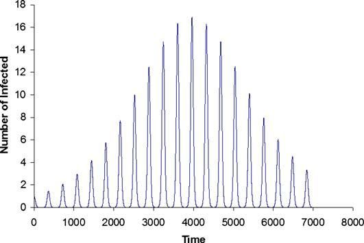
The threshold condition (Re=1) as expressed by the effective reproduction number, Re, in Eq.
(1-7) is now also a periodic function of time,
Re(t) = β(t)S(t)/(N(t)γ)
As R(t) > 1, the number of infected individuals (I) increases after a time delay. As Re(t) < 1,
the number of infected individuals decrease. Thus, as Re(t) varies periodically from below 1 to
over 1 within one year period, the infected individuals also varies periodically as shown in Fig.
4 based on Eqs. (1-6) and (2-14), a simulation done by Coutinho et al. (2006). In addition, the
maxima of I increase as the average (over one year) Re-avg(t) > 1 for the first 11 years and
decrease as the average Re-avg(t) < 1 after that.
Fig. 4. Simulation of a system with sinusoidal transmission rate (Coutinho et al., 2006). The time unit is in days.
2.3.2 A Modified SIR model – Humans, Vectors and Eggs
A more advanced Ross-Macdonald model to incorporate seasonal temperature variation is
given by Massad et al. (2011) & Coutinho et al. (2006). In this model, they have considered
three components in the dengue transmission process: humans, mosquitoes and their eggs
which include other intermediate stages like larvae and pupae. It is the mosquito eggs who
survive the winter. This component is necessary in the model in order to explain the observed
dengue phenomena: overwintering without assuming unreasonably high biting rate
(Coutinho et al., 2006).
The flow diagram is shown below which is created based on the mathematical equations
given by Massad et al. (2011) & Coutinho et al. (2006).
The relevant equations are those describing the changes of Infected humans (IH), Infected
female mosquitoes (IM), Infected eggs (IE), and latent mosquitoes (LM), although to solve the
equations, a full set of 9 differential equations are needed – one for each compartment and
- 19 -You can also read