Energy and Climate Economics - Munich, 4-5 March 2021 Motivation Crowding in Peer Effects: The Effect of Solar Subsidies on Green Power Purchases ...
←
→
Page content transcription
If your browser does not render page correctly, please read the page content below

Energy and Climate Economics
Munich, 4–5 March 2021

Motivation Crowding in Peer Effects: The Effect of
Solar Subsidies on Green Power Purchases
Andrea La Nauze

Motivation Crowding in Peer Effects: The Effect of
            Solar Subsidies on Green Power Purchases

                                       Andrea La Nauze∗

                                         March 3, 2021

                                             Abstract

           I test whether economic incentives dampen peer effects in public-good settings.

        I study how a visible and subsidized contribution to a public good (installing solar

        panels) affects peer contributions that are neither subsidized nor visible (electing

        green power). Exploiting spatial variation in the feasibility of installing solar pan-

        els, I find that panels increase voluntary purchases of green power by neighbors.

        However, using sharp changes in government incentives over time, I find that the

        magnitude of the spillover depends on the level of subsidies to solar. The results

        support the hypothesis that signals drive peer responses to visible public-good con-

        tributions, and that economic incentives blur those signals.

  ∗
      School of Economics, The University of Queensland, St Lucia, Queensland, Aus-
tralia. Email address: a.lanauze@uq.edu.au. I thank Todd Gerarden, Ken Gillingham,
Leslie Martin, Lise Vesterlund, Randy Walsh, and audience members at Carleton Univer-
sity, Pennsylvania State University, University of Queensland, Resources for the Future,
AERE Summer Conference, North East Workshop on Energy Policy and Environmental
Economics and Mid-West Energy Fest.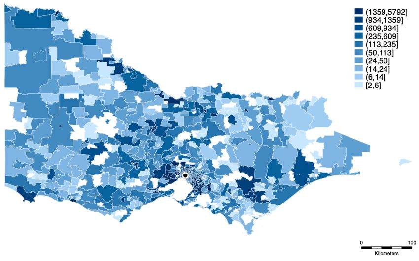
1     Introduction

Despite the economic incentive to free ride, public-good contributions are common. Indi-
viduals routinely give to charity, purchase ethical products and restrain their consumption
of goods with negative externalities. The discrepancy between economic incentives and
observed levels of prosocial behavior motivates research that aims to generate better
predictions of policy such as tax rebates and subsidies on public goods.
    From a theoretical standpoint, high rates of prosocial behavior challenge traditional
models, and motivate the search for alternatives. One such alternative incorporates the
notion of intrinsic, extrinsic and image rewards. Intrinsic rewards are the value to the
individual of being prosocial. Extrinsic motivations are material or monetary rewards
while image rewards are those that an individual gains from other people’s perception of
them as a prosocial type. Motivation crowding theory suggests that extrinsic incentives
may crowd out both intrinsic and image motivations. This theory is supported by em-
pirical evidence that economic incentives can discourage prosocial behavior (Gneezy and
Rustichini, 2000a,b; Mellström and Johannesson, 2008).
    Bénabou and Tirole (2006) argue that economic incentives may reduce prosocial be-
havior because the image value of a prosocial action is linked to intrinsic motivations
and is therefore compromised by other rewards. So if economic incentives make it more
likely an action is interpreted as arising from extrinsic motivation, then the actor is seen
as behaving less prosocially. In support of this mechanism, there is evidence from the
lab and the field that, when a giver’s actions are observable, visible economic incentives
reduce charitable contributions (Ariely et al., 2009).
    This paper explores a new mechanism by which economic incentives may reduce con-
tributions to public goods: peer behavior. Theories of conditional cooperation suggest
that people are more willing to act prosocially when others do so. These theories are
supported by evidence both from the lab and the field that peers affect charitable dona-
tions (Frey and Meier, 2004; Alpizar et al., 2008; Shang and Croson, 2009; Meer, 2011;
Jack and Recalde, 2015; Smith et al., 2015; Archambault et al., 2016; Kessler, 2017).
Less is known, however, about the role of motivation and signaling in generating these

                                             1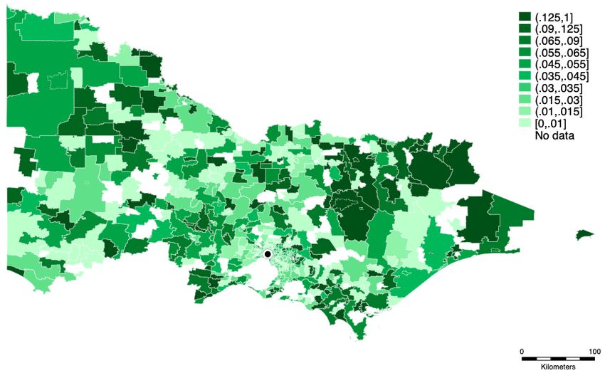
peer effects. Signaling one’s prosocial type may encourage peer contributions for example
by establishing norms for prosocial behavior or by creating peer pressure. If economic
incentives compromise the prosocial signal of a contribution then they may also reduce
peer contributions by lowering peer pressure. Such an effect would also be consistent with
evidence that donors avoid solicitations for charitable contributions (DellaVigna et al.,
2012; Andreoni et al., 2017) and exploit excuses such as uncertainty and moral wiggle
room to lower their contributions (Dana et al., 2007; Exley, 2015a,b).
   I test whether visible and subsidized prosocial behavior crowds in unobserved, un-
subsidized contributions from neighbors. The visible action is the installation of solar
panels. The private or unobserved action is electing to pay a premium for green power -
a voluntary program that increases the volume of renewable energy at the wholesale level.
Critically, the installation of solar panels is not only visible but is also heavily subsidized
while electing to buy green power is neither subsidized nor visible. In addition, subsidies
provided to the installers of solar panels fall dramatically over time so that the value of
extrinsic rewards and therefore the signaling value of an installation changes sharply at
discrete points in time.
   I study the effects of rooftop solar installation on voluntary purchases of accredited
green power in the state of Victoria, Australia over the period 2009 to 2016. The primary
data contain the full customer inventory for a single electricity retailer in the state.
I match each new contract to the number of solar panels installed in that postcode
using installation data from the Clean Energy Regulator. These data are well suited
to exploring the interaction between economic incentives and peer behavior. Australia
is the largest per capita market for rooftop solar in the world, with approximately one
in six dwellings having panels by the end of the sample period. In addition, there is
substantial variation across time and space in solar panel installation and the sample
period covers several sharp changes in the subsidies available. Critically, changes in the
subsidies were extremely well covered by major news outlets and further publicized by
significant marketing campaigns undertaken by solar installers.
   The empirical strategy is two fold. The first objective is to establish whether on
average, an additional solar panel in a neighborhood increases the probability that a

                                              2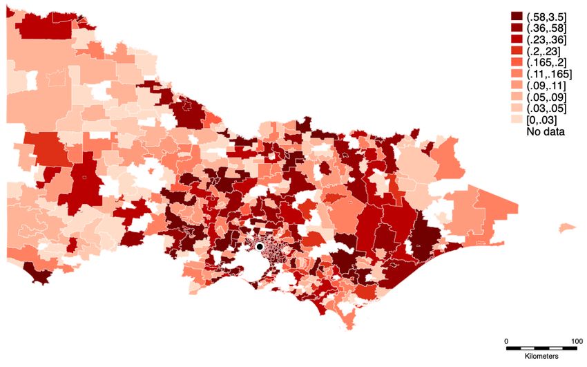
customer opts in to a green power plan. I exploit differences in the visibility of solar
panel adoption relative to green power contracting to overcome the classic problem of
reflection in the estimation of peer effects. I then combine cross sectional variation in
the cost of installing solar panels across houses with different roof materials, with time-
varying shocks in the global price of solar panel modules to develop an instrument for
neighborhood level installation. Specifically, I use variation across postcodes in the ratio
of metal to tile roofs and interact this with the inverse of a global solar module price
index. Using data from a pre period before the mass uptake of solar, I show that there
are parallel trends in green power purchasing in postcodes with above and below median
metal to tile roof ratios. I also show evidence for parallel trends in house prices across
postcodes by roof ratio.
   I find that, on average over the sample period, solar panel installation increases the
fraction of new contracts that are green power. An additional 100 dwellings with solar
panels increases the share of non-solar customers signing new green power contracts by
0.002 (mean share of green power contracts is 0.02). Thus a private, unobserved con-
tribution to an impure public good is crowded in by a visible peer contribution. There
are two main threats to identification. The first arises from differential trends across
neighborhoods via processes such as gentrification. A series of empirical exercises con-
trolling flexibly for heterogeneous time trends suggest that the results are robust to this
possibility. The second threat to identification comes from the possibility that the firm
markets its products differently across postcodes, for example, by targeting green power
deals at customers in neighborhoods with high solar penetration. I show however that
differences in marketing effort across postcodes do not explain the relationship between
solar panel installations and green power sign ups.
   I next establish that economic incentives interact with peer effects. To do so, I test
whether the impact of an additional solar panel in a high subsidy period is different to the
impact of an additional solar panel in low subsidy period. The identification strategy is
an event study design that relies on multiple sharp changes in subsidies over the period of
the sample. In event time, “high” subsidy periods are periods immediately after a subsidy
increase or before a subsidy decrease, and “low” subsidy periods are those immediately

                                             3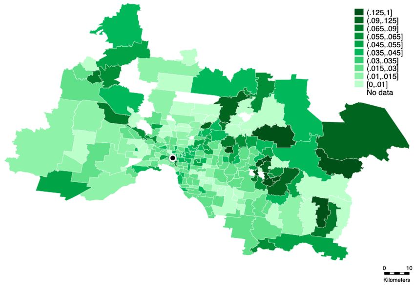
before a subsidy decrease or after a subsidy increase.
    I find that solar panels have a smaller crowd-in effect in high subsidy periods relative
to solar panels in low subsidy periods. This is consistent with the idea that extrinsic
incentives affect the signaling value of a prosocial action, and that this in turn drives
peer behavior.1 The results survive robustness checks that include adding controls, using
differences in roof type as an instrument, redefining the event window, dropping early
observations and restricting the sample to outer suburbs of the capital city. I also under-
take a series of three placebo tests to demonstrate that the event study effects are not
spurious.
    The primary contribution of this paper is to study whether economic incentives at-
tenuate peer effects in public-good settings. In doing so, it connects two related but
separate branches of literature on prosocial behavior. The primary concern of the first
branch of literature has been to establish the role of motivation, and in particular the role
of economic incentives in an individual’s propensity to act prosocially (Bénabou and Ti-
role, 2006; Ariely et al., 2009; Lacetera et al., 2012). Other contributions focus explicitly
on identifying the role of signaling in motivating prosocial behavior (Sexton and Sexton,
2014; Dubé et al., 2017). I add to this literature by considering how extrinsic incentives
may also affect the actions of this individual’s peers, who are implicitly the recipients of
any prosocial signals that are sent. The effect of peer behavior on contributions is the
focus of the second branch of literature.2 I demonstrate that the strength of the prosocial
signal delivered by a public-good contribution affects the magnitude of the subsequent
peer effect.

    1
        An alternative signaling explanation would be that during a high subsidy period a solar panel
sends a poorer signal about the installer’s belief about the quality of the public good (in this case, the
importance of reducing emissions to abate climate change). However, the size of the subsidy is itself a
quality signal.
    2
        This literature is fairly extensive but see, for example as cited above: Frey and Meier (2004);
Alpizar et al. (2008); Shang and Croson (2009); Meer (2011); Jack and Recalde (2015); Smith et al.
(2015); Archambault et al. (2016); Kessler (2017)

                                                    4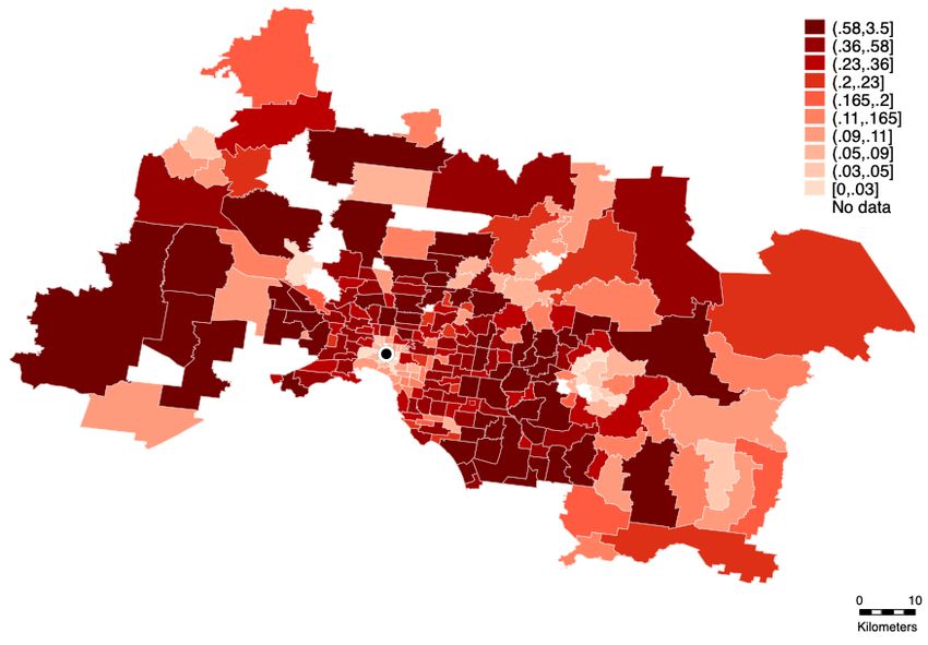
This paper also studies contributions to impure public goods and in particular the
effects of government incentives for environmentally friendly technologies (for a recent
study of impure public-good contributions see Kesternich et al., 2016). Outside of char-
itable donations, little is known about how peer behavior affects private, un-solicited
contributions to public goods. Bollinger and Gillingham (2012) and Kraft-Todd et al.
(2018), among others, find evidence that peers influence the diffusion of solar panels.
This diffusion could be the result of crowding in but it could equally reflect social learn-
ing about the private benefits of solar panels. Indeed Bollinger et al. (2020) show that
diffusion of dry landscaping for water conservation is stronger when there are financial
incentives to reduce water consumption.3 The effect of neighborhood solar installation on
peer green power purchases is not influenced by learning about private benefits of green
power, and is therefore more likely to be a pure prosocial spillover. Spillovers from solar
panel installation to intermediate outcomes such as votes for green parties and belief in
climate change have also been found in the literature (Comin and Rode, 2013; Beattie
et al., 2019).
    Finally, many papers study the effect of incentives on adoption of environmentally
friendly technologies (see Sallee, 2011; Huse and Lucinda, 2014; Boomhower and Davis,
2014; Hughes and Podolefsky, 2015, for example). In contrast to this literature, the focus
here is on how these incentives affect the prosocial contributions of an adopter’s peers.
From a policy perspective I show that accounting for peer responses decreases the cost
effectiveness of subsidies as a policy mechanism. I also demonstrate that subsidies may
not increase contributions to a public good even if adopters are marginal and that when
adopters are inframarginal, subsidies decrease contributions.
    The remainder of the paper is structured as follows. Section 2 provides context for

    3
        A related literature in environmental economics studies the role of social norms and peer comparisons
in energy and water consumption (Allcott, 2011; Ferraro and Price, 2013; Byrne et al., 2017). Relevant
papers in this literature study the interactions and relative effectiveness of price vs social norm treatments
(Pellerano et al., 2017; Ito et al., 2017) and the role of observability (Delmas and Lessem, 2014).

                                                       5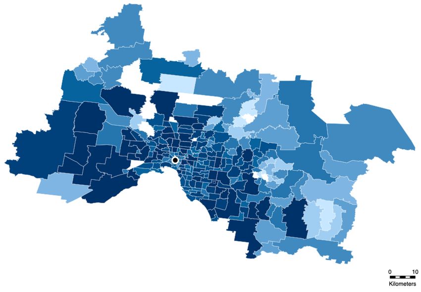
the study before Section 3 outlines the data in detail. Section 4 investigates whether
there is an average spillover from solar panels to green power adoption before Section 5
tests whether any spillover is affected by available subsidies. Section 6 discusses policy
implications and Section 7 concludes.

2        Background

The setting for this study is the state of Victoria in Australia over a period covering
the rapid adoption of rooftop solar. Figure 1 shows aggregate (state-level) trends in
rooftop solar using data from the Clean Energy Regulator.4 At the start of the sample
period there was very little solar installation. By the end of 2015, approximately one
in six households had installed solar panels on their roof. There are several reasons for
this rapid adoption including rising electricity prices, high levels of irradiance and the
subsidies available to installers.
    Table 1 reports the subsidies available over the study period. Explicit incentives to
install solar were provided by both federal and state governments.5 The federal gov-
ernment used two different mechanisms to subsidize rooftop solar. Initially, subsidies
took the form of a fixed rebate. In 2009, the government instead granted solar installers
the right to create Renewable Energy Certificates that obligated parties could use to
demonstrate compliance with the Mandatory Renewable Energy Target.6 As with grid

    4
        The Clean Energy Regulator is the Australian Government agency that administers the Renew-
able Energy Target. The data represent all solar panel installations claiming subsidies under Federal
Government programs.
    5
        Solar installers are also implicitly subsidized by avoiding some of the costs of the distribution network
that are recovered by per kWh charges on electricity consumption.
    6
        This scheme would be called a Renewable Portfolio Standard in the United States. The scheme is
designed to add renewable generation capacity to the grid. Obligated parties (retailers of electricity) are
required to surrender Renewable Energy Certificates equal to a proportion of their sales of electricity.
Renewable Energy Certificates can be created by eligible new renewable energy generators.

                                                         6
scale renewable energy installations, the number of certificates that could be created by
a solar installation was based on production potential. However to specifically support
small-scale installations, the government introduced a small scale multiplier for the first
1.5kW of capacity. From June 2009 to June 2011 this multiplier was 5. The multiplier
was reduced from 5 to 3 in July 2011, from 3 to 2 in July 2012 and was eliminated in
2013.
State governments also provided incentives to install solar panels by guaranteeing a
set feed-in tariff for electricity sold to the grid.7 Households are typically guaranteed
these feed-in tariffs for a fixed period of time, e.g. 10 years. Before 2009, the feed-in tariff
was a 1:1 match with the retail cost of electricity. From November 2009 the guaranteed
feed-in tariff increased to 60c/kWh, or roughly three times the retail cost of electricity at
the time. This feed-in tariff was reduced to 25c/kWh in late 2011, and reduced further
to 8c/kWh and then 6c/kWh in 2013 and 2014 respectively.
Figure 2 shows a back of the envelope net present value (NPV) calculation for a 3kW
solar installation over the study period assuming a 5% discount rate.8 In particular,
it shows a period where solar panels were a relatively attractive investment and large
changes in the private return to installing solar when subsidies change.
The study period also coincides with a steep decline in sales of green power. Alongside
the growth of rooftop solar, Figure 1 plots aggregate trends in green power purchases over
the sample period using data from the National Green Power Accreditation Program.9 In
Australia, customers can elect to purchase a green power product in a relatively mature
retail market for electricity. In this sector, retailers compete for customers by offering
7
These feed-in tariffs are referred to locally as net feed-in tariffs because they pay households for
electricity produced, net of the household’s own simultaneous consumption.
8
I take the calculations of NPV for installation of a solar panel in Victoria in 2015 in Wood and Blow-
ers (2015), and adjust it for changes in solar panel installation prices from the Australian Photovoltaic
Institute along with changes in subsidies. See Appendix B for further details on this calculation.
9
This program, administered by the New South Wales Government, is a joint government initiative
to promote renewable energy by increasing consumer confidence in accredited green power products.
7a variety of plans, including the option of purchasing a green power product that is
accredited by government. These products guarantee that a fixed amount, or stipulated
percentage of the consumer’s electricity consumption, will be sourced from renewable
electricity generators. Accredited green power products ensure there is no double counting
across mandatory and voluntary green power programs and use the “GreenPower” logo.10
Most retailers carry an accredited green power product.
Figure 1 shows a strong correlation between the rise of rooftop solar, and the drop in
household purchases of green power. There are several reasons that this correlation might
be observed. First, households may substitute from purchasing green power to installing
solar panels. Second, high levels of solar panel installation may crowd out public-good
contributions previously made by green power customers. Finally, the correlation may
be spurious or driven by some other time varying factor. Figure 1 also shows that at the
start of the sample period, when subsidies to solar panels are highest (2009-2011), the
decline in green power purchases is steepest. This is suggestive evidence that subsidies
to solar may also play a role in the declining popularity of green power. In the remainder
of the paper I outline an empirical strategy to identify the causal effect of neighborhood
installation on green power sign ups, and the causal effect of subsidies on the size of this
spillover.
For subsidies to solar panels to have an impact on green power purchases, it must be
that prospective green power purchasers (or at least some of them) were aware of these
subsidy changes. During the period of study climate change policy, renewable energy and
electricity prices were a frequent feature of news coverage and numerous media reports
at the time suggest that these subsidy changes were well publicized.11
10
In practice, to sell an accredited green power plan, retailers must demonstrate that they have
purchased sufficient Renewable Energy Certificates to cover their sales of green power products in addition
to their mandatory obligations.
11
See for example the following articles published in national media outlets over 2010-2012: Sid Maher
‘Greg Combet takes heat out of solar scheme’, The Australian December 1 2010 ; Sid Maher ‘Combet cools
on solar credits’ The Australian May 5 2011 ; Naomi Woodley, ‘Government reducing solar subsidies’
83 Conceptual Framework
To consider the overall impact of subsidies on the public good of emissions reductions,
consider a simple model of the emissions of an individual (Ei ) who consumes ki kiloWatt
hours (kWh) of electricity. Assume this individual can make two choices to affect their
overall emissions: they can either purchase green power (gi ), or they can choose to install
solar panels (si ). For simplicity consider the case where each decision is binary such that
(gi , si ∈ {0, 1}):
Ei = (1 − γgi )βki − ψsi
where β is the average emissions intensity of the grid, γ is the proportion of the consumer’s
electricity that is procured as green power, and ψ is the average emissions displaced by a
solar panel installation. We wish to understand how this consumer’s emissions change as
∂Ei
the subsidy for solar panel installation changes, i.e. we wish to understand ∂f
where f
is the subsidy to solar installers. This subsidy has three potential impacts. First, it will
affect the likelihood of the consumer adopting panels. Second, if adopting solar panels
and purchasing green power are substitutes, then the subsidy will also have an effect on
green power purchases via this substitution. Finally, if there are spillovers, or peer effects,
the subsidy may have additional effects on the consumer via the installation decisions of
others. To formalize, suppose that the green power decision depends on an individual’s
own solar adoption choice, the adoption choice of their neighbors, and the subsidy, and
takes the following form:
gi (fi ) = h(si (f )) + ρ(f ) × l(s−i (f ))
where s−i are the installation decisions of neighbors and ρ(f ) allows the spillover from a
neighbor’s installation to be a function of the subsidy level. Then the quantity of interest
ABC Dec 1 2010 ; ABC NEWS, ‘Solar panel subsidies scrapped early’ ABC 16 Nov 2012
9is:
∂Ei
= −βγki h0 (si )s0i (f ) + ρ0 (f )l(s−i (f )) + ρ(f )l0 (s−i (f ))s0−i (f ) − ψs0i (f )
∂f
Re-arranging:
∂Ei
= −s0i (f ) [βγki h0 (si ) + ψ] − βγki ρ0 (f )l(s−i (f )) + ρ(f )l0 (s−i (f ))s0−i (f )
∂f | {z } | {z }
Substitution effect Crowding effect
The first term is the net impact of substitution within the household from green power
to solar panels. Substitution implies that h0 (si ) < 0. The second term is the net impact
of crowding, its sign depends on the elasticity of solar installation to the subsidy (s0−i (f ))
and the change in the spillover due to the subsidy (ρ0 (f )). The aim of this paper is to
provide empirical evidence for the sign and magnitude of ρ0 (f ). If it is negative then
higher subsidies reduce the spillover effect. The average crowding effect then depends on
relative magnitudes.12
In general, if technology adopters are marginal to subsidies, i.e. subsidies cause a
substantial portion of adoption, then they are less likely to eliminate positive spillovers
to public-good contributions. On the other hand, if adopters are inframarginal, such
that they would have adopted in the absence of the subsidies (i.e. s0−i (f ) = 0), then
subsidies on net have a negative impact on public-good contributions. Boomhower and
Davis (2014) suggest that a non-negligible number of technology adopters may be in-
framarginal. Even in the absence of spillovers, inframarginal adopters can compromise
program cost-effectiveness. If they also lead to crowd out, subsidies would become even
less cost-effective. Further, even if the crowding effect at the individual level is small, if
the peer group is large, the net impact of crowding may be substantial. This considera-
12
In practice the literature on peer effects suggests that there are spillovers from solar adoption to
peer solar adoption (Bollinger and Gillingham, 2012). These spillovers are also feasibly related to the
size of subsidies (Bollinger et al., 2020).
10tion is particularly important in a policy environment that appears to favor policies such
as technology subsidies over externality pricing. The results also have implications for
the charity sector, and in particular for fundraising that rewards donors for their contri-
butions with gifts. If these gifts are seen as a valuable private benefit associated with the
contribution, they may in turn lower peer contributions.
4 Data
To identify the causal relationship between solar panels and green power purchases I
use customer-level data on plan choice for a small-medium size electricity retailer in the
contestable retail market in the state of Victoria. The data contain the full inventory
of customers over the period 2006-2016. For approximately 300,000 the data include
plan choice, contract start dates, and billing data. I exclude customers who have or
adopt solar panels at any point from 2006-2016 and use billing and plan choice data to
identify whether a household purchases green power.13 The distribution of customers
at the postcode level over the state and within the capital city Melbourne is shown in
Appendix Figure A1. The sample is drawn from across the state with more customers in
the more densely-populated region of Melbourne.
I aggregate the customer data to the postcode-quarter level then match it to solar
penetration data from the Clean Energy Regulator. I also match postcodes to 2006, 2011
and 2016 census data from the Australian Bureau of Statistics14 and postcode-quarter
house and unit sales data for 2000-2016 from the Victorian Government Department of
Environment, Land, Water and Planning. To construct the instrument I use a time in-
variant measure of roof materials by postcode from GeoScience Australia. Roof material
data come from the National Exposure Information System (NEXIS). GeoScience Aus-
13
Including solar adopters and controlling for their adoption decision does not however change the
results. As the vast majority of green power customers opt for the lowest level of green power I analyze
the extensive rather than the intensive margin.
14
Census data are interpolated to construct variables at the quarterly frequency.
11tralia collects data for NEXIS from Local Government Authorities, the Victorian Census
of Land Use and Employment, Victoria’s Office of the Valuer-General and GeoScience
Australia building and disaster surveys.15 The instrument also uses a global price index
for solar modules from Bloomberg New Energy Finance.16 Appendix Figure A2 plots the
value of this index during the sample period.
Table 2 provides summary statistics of the key variables of interest over the study
period. As the module price index is only available from 2009, the study period is 2009-
2016. Appendix Table A1 provides summary statistics for the same variables over the full
period 2006-2016. The share of customers signing green power contracts over 2006-2009
is significantly higher than the later period, reflecting trends in green power purchasing
over time. In the following section, trends in green power purchases prior to 2009 will be
used to provide evidence for identification.
Appendix Figure A3 shows the distribution of green power and solar panels in the
sample across the state while Appendix Figure A4 shows the distribution within the
capital city Melbourne. Unsurprisingly, solar panels are least prevalent in the city and in
particular in the denser inner suburbs where shading and smaller roof sizes make them
less suited to solar panel installation.
Figure 3 plots the share of new contracts that are green power for the sample used
in this paper. The trends are very similar to the aggregate (state level) trends in Figure
1. As noted, this sample excludes solar households. Hence among non solar households
for this single retailer, and among customers signing new contracts, there is still a strong
correlation between the rate at which customers sign contracts for green power, and
the rate at which new solar panels are installed. If this relationship were causal, it
15
GeoScience Australia states that where building specific data are not available it is predicted based
on settlement type.
16
To construct this index, Bloomberg collects quotes from buyers, sellers and traders of modules and
module components such as silicon. Following a quality control process, these data are then averaged
and published as an Index.
12would suggest that solar panels crowd out public-good contributions via a reduction in
the number of consumers willing to purchase green power. However other time-varying
factors, such as trends in the cost of purchasing electricity and reductions in solar module
costs, may be driving this correlation. Again, the figure also provides suggestive evidence
for the relationship between economic incentives and spillovers. In particular, the decline
in green power purchases is steepest at the time that subsidies are highest.
To identify the causal impact of solar panels on green power purchases I use cross
sectional variation in the feasibility of installation, along with plausibly exogenous time
variation in the cost of modules. This research design exploits the fact that solar panel
installation is more feasible in neighborhoods that contain more houses with metal roofing
materials as installing panels on metal sheeting is both easier and less costly than other
materials such as tile.
Figure 4 shows the difference in solar panel adoption and green power purchases across
postcodes with above vs below median number of houses with metal relative to tile roofs.
At the start of the sample, there is no difference in the number of solar installations, by
the end of the sample they have more solar installations. At the start of the sample, the
percentage of customers in these postcodes opting in to green power is also lower (though
noisy) and by the end of the sample the gap in green power purchases has disappeared.
5 Do Solar Panels Affect Neighbors’ Green Power
Choice?
5.1 Empirical Strategy
The first empirical objective of this paper is to establish whether an additional solar panel
in a postcode impacts the probability that a non-solar customer in that postcode signs
a contract for greener electricity. Hence at the postcode level I wish to identify β in the
following regression:
Green P owerit = αi + ρt + βSolar Roof topsit + it (1)
13where Green P owerit is the proportion of households in postcode i that commence a
contract in period t that opt in to green power, αi are postcode fixed effects, ρt are
quarter-year fixed effects and Solar Roof topsit is the number of solar panels installed in
postcode i by time t. The parameter of interest β measures the effect of an additional
solar installation on the fraction of new contracts in a postcode that opt in to green
power.
The parameter β is a peer effect. Ordinarily, identification of peer effects is compli-
cated by the reflection problem, or an inability to distinguish the direction of influence
between peers (Manski, 1993). Here, I exploit differences in the visibility of actions to
argue that the direction of causality runs from Solar Roof topsit to Green P owerit and
not the reverse. Unlike solar panels, decisions to sign up to green power are private,
and not observed by neighbors. It is therefore unlikely that one neighbor’s choice to buy
green power influences another’s choice to install solar panels. On the other hand, solar
panels have been shown to affect neighbor’s beliefs in climate change, and their likelihood
of voting for a green party (Comin and Rode, 2013; Beattie et al., 2019). In addition,
there is a considerable lag between the decision to adopt solar and the installation of
solar panels. This lag suggests that solar panels observed at time t are unlikely to be
influenced by green power sign ups at time t.
A remaining concern with estimating equation 1 is that Solar Roof topsit is not ran-
domly assigned across postcodes. An OLS estimate of β may therefore suffer from omitted
variable bias for example due to unobserved shocks to environmental preferences arising
from something like a local campaign that lead to both solar installation and green
power purchases. To address this identification problem, I exploit variation across neigh-
borhoods in how feasible it is to install solar panels based on the average type of roofing
in a postcode.
In Australia, approximately 75% of houses have roofs made of metal sheeting, 20%
have roofs of tile (either concrete or terracotta) and the remainder use materials such
as concrete or fiber cement. I exploit postcode level differences in the number of metal
roofs relative to the number of tiled roofs. The logic of the research design is as follows:
suppose there are two similar neighborhoods, however one has relatively more houses with
14tiled roofs (control) and the other has relatively more houses with roofs of metal sheeting
(treatment). Because it is cheaper to install solar panels on roofs with metal sheeting,
it is more suited to solar panel installation. Identification then relies on there being no
unobserved time-varying differences across these two neighborhoods that are correlated
with changes in environmental preferences that might simultaneously drive solar panel
installation and green power purchases.
The fact that the decision of roofing material is a long term investment suggests that
average roofing materials in a neighborhood are unlikely to respond to short term fluctua-
tions in neighborhood composition. The decision of roofing material is also itself unlikely
to be driven by trends in environmental concern or by factors correlated with environmen-
tal concern. For example, if metal roofs were substantially more thermally efficient we
might expect suburbs with greener preferences to have a higher proportion of metal roofs.
However neither roofing material has significant thermal insulation properties. Further,
on average, the lifetime costs of metal and tiled roofs do not differ substantially.17 While
metal roofing has greater fire safety and is a more versatile roofing material than tile
it is also noisier and less durable. It therefore seems plausible that there is no causal
relationship between shocks environmental preferences and average neighborhood roofing
materials.18
Even if there is no causal relationship between environmental preferences and roof
type, it is still possible that roofing materials are correlated with unobserved changes in
17
The installation costs of concrete tile are generally lower than that of metal sheeting which are in
turn lower than terracotta tile.
18
It is also possible that people choose to install panels when they put on a new roof, and given the
cost differences in panel installation across metal and tile, they may choose to install a metal roof. If
solar panel installation causes roof type then roof type is not a valid instrument. Ideally I would therefore
use differences in roof type before 2009. Unfortunately the NEXIS data do not provide any information
on the vintage of roofs in a suburb. However roofs can last up to 50 years so re-roofing is a fairly rare
event. In addition, I exploit a time invariant measure of roof type at the neighborhood level so that
identification does not come from changes in roof type over the sample period.
15environmental preferences. This might be the case, for example, if tiled roofs are more
popular in suburbs with older houses, and neighborhoods with older houses are more
likely to undergo gentrification as they are closer to the inner city. In practice both
roofing materials have been in common use since the 1850s, or shortly after the capital
city of Melbourne was founded. Appendix Figure A5 shows examples of the mixed use
of tile and metal sheeting within classic inner city Victorian terraces and within more
modern suburban developments. Nevertheless, to address the concern about vintage and
gentrification within the inner city, I separate the sample by distance from the center of
the city, and re-estimate the parameters for inner, middle and outer suburbs of Melbourne.
I use a measure of neighborhood roof suitability to develop an instrument for the
change over time in the number of solar installations in a postcode. To construct the
instrument I interact a time-invariant variable at the local level (cross sectional variation
in roof type) with a common trend variable (time variation in the cost of solar panel
modules). To account for differences in scale, I multiply the ratio of metal to tile roofs
by a time invariant measure of the number of dwellings.19 The instrument Zit is defined
in equation 2.
M etali Roof si
Zit = (2)
T ilei M odule P ricet
M etali
where T ilei
and Roof si are time-invariant measures of the ratio of metal to tile roofs
and the number of roofs in postcode i respectively. The distribution of the time invariant
component of the instrument is plotted in Appendix Figure A6. The top map shows
variation across the state. The bottom map shows variation in the capital city Melbourne,
where over 75% of the state’s population reside. There is considerable variation in the
19
Accounting for scale improves the strength of the instrument because the endogenous variable is
cumulative solar rooftops. The construction of the instrument effectively penalizes suburbs with the
same number of metal roofs, but a higher number of tile roofs, and also penalizes suburbs with the same
ratio of metal to tile roofs but a smaller number of total roofs. Using the percentage or number of metal
roofs leads to similar conclusions, but the instrument is weaker.
16value of the instrument across the state, within the capital city, and within suburbs that
are approximately equi-distant from the center of the capital city. The time varying
component of the instrument, M odule P ricet , is the global solar panel module price
index at time t and is plotted in Appendix Figure A2. I use the inverse of the module
price to ensure that increases in the value of the instrument are associated with increases
in the endogenous variable Solar Roof topsit .
5.1.1 Testing for Parallel Pretrends
The exclusion restriction requires that there is no direct effect of postcode average roofing
material on the probability that a customer without solar panels signs up to green power.20
This would appear to be a plausible assumption. Identification also relies on shocks
to environmental preferences being orthogonal to the ratio of metal to tile roofing in
a neighborhood. If neighborhoods with a high metal to tile ratio differ due to time
invariant characteristics, then these are captured in postcode fixed effects αi . However, if
time-varying processes such as uneven gentrification are more likely to occur in postcodes
with a high number of metal roofs and these processes cause an increase in green power
purchases then the estimates would be biased.
The key identifying assumption is parallel trends in green power purchasing across
neighborhoods with different roof ratios. Column (1) of Table 3 shows that in the period
before the uptake of solar panels (2006-2009), there is no evidence of differential trends
across postcodes with more metal roofs. Column (2) shows that in the period after the
rapid uptake of solar panels, green power purchases increased in postcodes with a high
proportion of metal roofs relative to those with a high proportion of tile roofs. This is
20
If solar and green power are substitutes it is possible that households in neighborhoods that are less
suited to solar panel installation are more likely to purchase green power. This would cause a negative
correlation between roof ratio and green power purchases and go against finding a crowd in effect. I
explore this possibility below and show in Appendix Table A13 that accounting for households who
switch to solar does not change the effects. For reference Table A5 shows the results at the household
level excluding solar households.
17consistent with a crowd in effect and also evident in the trend in Figure 4. Column (3)
shows average trends over the period 2009-2016 while Column (4) shows trends by period
and roof ratio in a fully interacted model over the period 2009-2016. Again, there is no
evidence for differential trends in green power purchasing prior to 2009, when solar panel
penetration began to rise more significantly in postcodes with a higher metal roof ratio.
Appendix Table A2 also demonstrates that there are no differential trends in other
characteristics of electricity contracts across neighborhoods with different roof ratios.
Column (1) shows that there are no differences in trends in the share of customers who
elect to pay their bill manually (the alternative being an automatic debit). Column (2)
shows that there are no differences in the share of customers that are eligible for a low
income concession.
One concern with this evidence is that there is limited pre-period data available
for testing pre-trends. As further supporting evidence therefore, Figure A7 plots the
difference in house price from 2000-2015 across neighborhoods with a relatively high
versus low metal to tile roof ratio. There is no statistically significant difference in house
prices. Appendix Table A3 reports estimated trends in house prices in the pre and post
2009 period by metal roof ratio. Again, there is no evidence that there are differential
trends. In the analysis I also demonstrate that changes to the set of time-varying controls
Xit that would be correlated with time-varying processes such as gentrification do not
significantly affect the magnitude of the estimate of β. As outlined below, I also allow for
flexible time trends by distance from the center of the city and restrict the sample based
on distance from the city, a proxy for vintage of houses and gentrification.
5.2 Results
Table 4 reports estimates of the average effect of neighborhood level solar panel installa-
tion on green power purchases using a straight fixed effects model. All standard errors
are clustered at the postcode level and the regression is weighted by number of customers
to account for aggregation. I find that an additional 1000 solar panels increases the frac-
tion of new contracts in a postcode that opt in to green power by approximately 0.02.
In Column (2) I use a LASSO to select observable neighborhood characteristics as con-
18trols. The LASSO selects four out of nine covariates: median income, median mortgage
payment, percentage with a bachelor’s degree and percentage employed full time. The
estimated effect is no different to the effect in Column 1.
Equation 1 imposes a linear relationship between the number of solar panels in a
postcode and the share of new contracts that contain green power, yet there is no clear
theoretical or empirical reason why the relationship should be linear, or that panels out-
side the arbitrary borders of a postcode but nearby would not have an impact on the
share of customers electing to purchase green power. Columns (3) - (6) impose alter-
native assumptions on the relationship between solar panels and green power purchases.
Regardless of the model of behavior assumed, on average a solar panel continues to have
a positive effect on green power sign ups. For example, Column (3) allows the effect of
solar rooftops to be nonlinear, demonstrating a diminishing effect as the installed base
increases, though the average effect of a solar panel is approximately unchanged from the
linear specification. Columns (4) and (5) report results of alternative models where the
measure of exposure to solar panels is panels per rooftop (Column (4)) and where the
measure of exposure to solar panels is panels per unit area (Column (5)). Once again,
I find a significant crowd in effect. Finally in column (6) I explore whether panels in a
municipality (but not in the postcode) also have a small crowd in effect on green power
purchases. I approximate municipality using the Statistical Area Level 3 (SA3) identi-
fier from the Australian Bureau of Statistics (ABS) Statistical Geography.21 I find that
panels within the municipality do crowd in green power purchases though this effect is
much smaller than the effect of within-postcode panels. This result is also comforting for
identification, as it suggests that the estimates are not driven by confounding trends at
the municipality level.
So far the relationship between solar panels and green power has been estimated in a
fixed effects setting. Table 5 reports estimates employing the instrument based on roof
ratio. Exploiting variation based on roof type does very little to change the magnitude
21
An SA3 consists of between 30,000 and 130,000 people and aligns closely to municipal boundaries.
19of the estimated impact of a rooftop solar panel. In Column (1) the estimated effect is
0.029, which is statistically indistinguishable from the estimate in Column (1) of Table
4. Controlling for neighborhood characteristics (Column (2)) again does not change
the estimated effect. Table 5 also reports F statistics for the first stage regressions,
demonstrating that the instruments are strong. First stage coefficients are reported in
Appendix Table A4.
There are two main threats to identification in the instrumental variables model. The
first comes from the possibility of non-parallel trends, or persistent shocks to green-power
purchases in postcodes with high metal to tile roof ratios, for example trends arising from
gentrification. To account for threats such as gentrification, I explore the robustness of
the results to the inclusion of a series of flexible time effects at the yearly level. First,
Column (3) of Table 5 reports results employing year by region fixed effects, where region
is again SA3 from the ABS. The results are robust to the inclusion of these fixed effects
and therefore to flexible time trends at the municipal level.
Columns (4)-(6) of Table 5 reports results allowing for a number of other flexible
time trends. In Melbourne, gentrification is most likely to occur in inner city suburbs.
Distance to the city center is therefore a proxy for likelihood of gentrification. Column (4)
of Table 5 demonstrates robustness to controlling for linear distance from the Melbourne
General Post Office in the city center separately for each year. Column (5) shows that
the effect of solar panels on green power purchases is robust to including an interaction
between Year fixed effects and an indicator for above median roof ratio, while column (6)
shows that the effect is robust to an interaction between Year fixed effects and quintiles
of roof ratio.
Finally Table 6 reports results from restricting the sample to Melbourne (column 1)
and then restricting to the inner city, middle suburbs, and outer suburbs of Melbourne.
Inner city suburbs are those within 5km of Melbourne General Post Office, middle suburbs
are between 5 and 20 km and outer suburbs are those greater than 20 km but still within
the borders of the city according to the Australian census boundaries. Appendix Figure
A8 maps these sample restrictions and the distribution of the time-invariant (scaled
roof ratio) component of the instrument. There are no significant effects either for the
20inner or outer suburbs, however the effect for middle suburbs is positive and statistically
significant. Thus most of the average effect seems to be driven by the behavior of those
residing in the middle suburbs of Melbourne, suburbs that are unlikely to be experiencing
the kind of gentrification that is a threat to identification.
The second main threat to identification comes from the possibility that the firm
engages in differential marketing activities across postcodes that are correlated with solar
panel installation. For example, if the firm takes observable solar panel installation as a
signal of the green preferences of people in a neighborhood, they may target green power
plans at households in that neighborhood. Then the observation that the share of green
power is higher in neighborhoods with more solar panels is in part driven by differences
in marketing. Several facts suggest that this is not a strong possibility: I find that the
results are robust to a variety of rich fixed effects including municipality × year effects
and to controls for distance from the city × year effects. To confound these estimates,
marketing efforts would have to be both be postcode specific and changing over time
with the installed solar base. This level of targeting does not seem consistent with the
marketing strategies of electricity retailers in the state, who, anecdotally, tend to target
larger geographic areas such as the “South East”.
To address any remaining concern presented by differential marketing efforts, I exploit
unique data on how customers were acquired by the company. In the customer inventory,
for the vast majority of customers (98%) I observe whether new contracts are the result
of telesales, door-to-door sales, a price comparison website, connection service or whether
the customer is renewing an existing contract. I group sales channels into three categories:
sales driven acquisitions (e.g. door-to-door sales which are the result of heavy and tar-
geted marketing effort), customer driven acquisitions (e.g. customers signing contracts
via a price comparison website who may be responsive to indirect marketing but were not
acquired by direct marketing efforts) and renewal customers.22 In Table 7 I show that
22
Appendix Figures A9 show the proportion of all new contracts by channel, and the total number of
new contracts by channel over the sample period
21the results are robust to controlling for the share of customers in a postcode acquired via
these direct (“Sales Driven Acquisition”) and indirect (“Customer Driven Acquisition”)
marketing efforts. Relative to renewal customers, a higher share of customers acquired
via direct or indirect marketing efforts is associated with a higher share of green power
contracts, however the effect of solar panels on green power purchases is unchanged.
6 Do Incentives Attenuate Peer Effects?
6.1 Empirical Strategy
Overall, the results summarized in the previous section suggest that a solar panel in
a neighborhood increases the likelihood that non-solar peers sign up to a green power
contract. The second empirical objective of this paper is to identify whether economic
incentives, or extrinsic motivations, have an impact on the peer effect from solar panel
installation to green power purchasing. To do so, I exploit sharp changes in solar subsidies
to test the hypothesis that peer effects depend on the level of subsidies available to solar
installers. I use these changes in subsidies in two ways. First, I separate the sample period
into three periods representing a high subsidy period (up to the first quarter of 2011), a
period in which subsidies were falling (from the first quarter of 2011 to the first quarter
of 2013), and a low subsidy period (after the first quarter of 2013). I then estimate the
effect of a solar panel in each of these periods by interacting an indicator for subsidy
period with the number of solar panels in equation 1.
The second approach is to use an event study framework. In this approach I will
estimate the following equation at the postcode level:
W
X
Green P owerit = αi + ρt + θτ (Solar Roof topsiτ × Event P eriodτ ) + it (3)
τ =−W
where Solar Roof topsiτ is the number of solar rooftops in event period τ and Event P eriodτ
is an indicator for being event period τ within the event window W . I normalize event
time such that τ ≥ 0 are high subsidy periods and τ < 0 are low subsidy periods. Thus
the quarter immediately before a subsidy increase is event period τ = −1 and the quar-
22ter immediately after a subsidy increase is event period τ = 1. Because there are both
increases and decreases in subsidies observed within the sample, the quarter immediately
before a subsidy decrease is also event period τ = 1. Because the events are overlap-
ping within the event window, an individual quarter may be both two periods before a
subsidy decrease, and one period after a subsidy increase. In this case, event indicators
Event P eriodτ =2 and Event P eriodτ =1 are “switched on”.23 Coefficients θτ therefore
measure the effect of an additional solar panel on purchases of green power in low (τ < 0)
and high (τ > 0) subsidy periods relative to periods outside the event window.24
To estimate the impact of subsidies, I compare θτ coefficients in periods immediately
before and immediately after a subsidy change.25 If incentives do attenuate the peer effect
then θτ |τ θτ |τ >0 . The identifying assumption is that other unobserved time-varying
factors that affect green power purchases and that are correlated with solar installation
do not change sharply with subsidies for solar panels. For the results to be spurious, some
other factor would have to cause the same pattern of changes in green power purchases at
exactly the same points in time as subsidy changes.26 Note also that although event time
is coded as positive for high subsidy periods, subsidies are declining over the period of the
sample. This, and the fact that Solar Roof tops is a cumulative variable, ensures that
the specification is not conflating the impact of a higher subsidy on the peer effect with
23
Appendix Figure A10 shows that the share of observations in each Event Period is relatively con-
stant. Appendix Table A6 shows that the number of observations that coincide with more than one
Event Period.
24
Appendix Table A6 shows that 20% of observations are outside the Event Window. Observations
outside the window are from first quarter of 2015. Dropping these observations does not change the
conclusions.
25
There is no cross sectional variation in available subsidies, instead, cross sectional variation comes
from differences in the number of solar rooftops in a postcode
26
Mian and Sufi (2012) use a similar research design to identify the effects of the Cash for Clunkers
stimulus program on auto purchases. They measure exposure to the program as the number of “clunkers”
(less fuel efficient vehicles eligible for trade-in subsidies) in a city before the stimulus came into effect.
23a non-linearity in the effect of Solar Roof tops on green power purchases. Furthermore
controlling for a quadratic in Solar Roof tops does not change the main findings.
To lend support to the results I employ two additional strategies. First, I include
time-varying controls in the event study estimation and demonstrate no change to the
main findings. Second, I also instrument for solar rooftops with the same instrument as
above where for each event interaction (Solar Roof topsiτ × Event P eriodτ ) I construct
an instrument (Ziτ × Event P eriodτ ).
6.2 Results
Figure 5 shows how the effect of solar panels on the likelihood a customer signs a green
power contract depends on subsidies in the quarter in which the contract is being signed.
In particular, it shows that an additional solar panel crowds in purchases of green power
when subsidies are low or declining, but an additional solar panel crowds out purchases
of green power when subsidies are high.
I next estimate equation 3 employing an event window of 18 months (9 months or 3
quarters on either side of the event). Coefficients and 95% confidence intervals for θ̂τ in
the linear fixed effects model are plotted in Figure 6 while coefficients and standard errors
are reported in column (1) of Table 8. As with the average effect estimates, regressions are
weighted by number of customers and standard errors are clustered at the postcode level.
The coefficients for τ < 0 are the effect of a solar panel in a low subsidy period. Similarly,
the coefficients where τ > 0 are the effect of a solar panel in a high subsidy period. On
average, I find that the effect of an additional solar panel during a high subsidy period
is lower than the effect of an additional solar panel in a low subsidy period.
I find very similar results when using the roof ratio instrument, and adding controls.
Figure 7 plots the reduced form and instrumental variables estimates for the event study
coefficients employing the roof ratio instrument interacted with event study indicators
as instruments. Figure 10 shows the reduced form and instrumental variables estimates
when controlling for the same time varying coefficients as Table 4. Coefficients and
standard errors for these event study coefficients are reported in Table 8.
Across all columns of Table 8 I find that the effect of a solar panel in a low subsidy
24You can also read