Impact of forcing on sublimation simulations for a high mountain catchment in the semiarid Andes - The Cryosphere
←
→
Page content transcription
If your browser does not render page correctly, please read the page content below
The Cryosphere, 14, 147–163, 2020
https://doi.org/10.5194/tc-14-147-2020
© Author(s) 2020. This work is distributed under
the Creative Commons Attribution 4.0 License.

Impact of forcing on sublimation simulations for a high mountain
catchment in the semiarid Andes
Marion Réveillet1,a , Shelley MacDonell1 , Simon Gascoin2 , Christophe Kinnard3 , Stef Lhermitte4 , and Nicole Schaffer1
1 Centro de Estudios Avanzados en Zonas Áridas (CEAZA), ULS-Campus Andrés Bello, Raúl Britan 1305, La Serena, Chile
2 Centre d’Etudes Spatiales de la Biosphère (CESBIO), Université de Toulouse, CNRS/CNES/IRD/INRA/UPS,
31400 Toulouse, France
3 Département des Sciences de l’Environnement, Université du Québec à Trois-Rivières, 3351 Boul. des Forges,

Trois-Rivières, QC, G9A5H7, Canada
4 Department of Geoscience & Remote Sensing, Delft University of Technology, Delft, the Netherlands
a now at: Univ. Grenoble Alpes, Université de Toulouse, Météo-France, CNRS, CNRM, Centre d’Etudes de la Neige,

38000 Grenoble, France

Correspondence: Marion Réveillet (marion.reveillet@meteo.fr)

Received: 8 February 2019 – Discussion started: 28 February 2019
Revised: 3 October 2019 – Accepted: 9 October 2019 – Published: 17 January 2020

Abstract. In the semiarid Andes of Chile, farmers and in-       pared to AWS. Therefore, the use of WRF model output in
dustry in the cordillera lowlands depend on water from          such environments must be carefully adjusted so as to re-
snowmelt, as annual rainfall is insufficient to meet their      duce errors caused by inherent bias in the model data. For
needs. Despite the importance of snow cover for water re-       both input datasets, the simulations indicate a similar subli-
sources in this region, understanding of snow depth distribu-   mation fraction for both study years, but ratios of sublimation
tion and snow mass balance is limited. Whilst the effect of     to melt vary with elevation as melt rates decrease with eleva-
wind on snow cover pattern distribution has been assessed,      tion due to decreasing temperatures. Finally results indicate
the relative importance of melt versus sublimation has only     that snow persistence during the spring period decreases the
been studied at the point scale over one catchment. Analyz-     ratio of sublimation due to higher melt rates.
ing relative ablation rates and evaluating uncertainties are
critical for understanding snow depth sensitivity to varia-
tions in climate and simulating the evolution of the snow-
pack over a larger area and over time. Using a distributed      1   Introduction
snowpack model (SnowModel), this study aims to simulate
melt and sublimation rates over the instrumented watershed      In the semiarid Andes, glaciers and seasonal snow cover are
of La Laguna (513 km2 , 3150–5630 m a.s.l., 30◦ S, 70◦ W),      the dominant water sources, as rainfall is episodic and in-
during two hydrologically contrasting years (i.e., dry vs.      sufficient to meet user demand. The region is characterized
wet). The model is calibrated and forced with meteorolog-       by very low precipitation amounts that are largely limited
ical data from nine Automatic Weather Stations (AWSs) lo-       to winter months (i.e., June, July and August) and are er-
cated in the watershed and atmospheric simulation outputs       ratic. Large interannual variability is observed, as the area is
from the Weather Research and Forecasting (WRF) model.          strongly affected by El Niño–Southern Oscillation (ENSO)
Results of simulations indicate first a large uncertainty in    (e.g., Falvey and Garreaud, 2007; Garreaud, 2009; Monte-
sublimation-to-melt ratios depending on the forcing as the      cinos et al., 2000). In broad terms, during El Niño periods
WRF data have a cold bias and overestimate precipitation        the semiarid Andes are characterized by warm air tempera-
in this region. These input differences cause a doubling of     tures and higher precipitation totals, whereas La Niña peri-
the sublimation-to-melt ratio using WRF forcing inputs com-     ods are on average colder with less precipitation (e.g., Ducan
                                                                et al., 2009). Whilst snowmelt comprises the bulk of avail-

Published by Copernicus Publications on behalf of the European Geosciences Union.
148                                                          M. Réveillet et al.: Impact of forcing on sublimation simulations

able water (Favier et al., 2009), due to low humidity, high
solar radiation and strong winds, sublimation is a significant
ablation process, especially at high elevations (Ginot et al.,
2001; Gascoin et al., 2013; MacDonell et al., 2013a). Conse-
quently, quantifying snow mass balance processes is crucial
for predicting current water supply rates and for informing
future projections.
   Despite the importance of snow cover for water resources
in this region, there is currently a limited understanding of
snow depth distribution and mass balance, largely due to the
difficulty of accurately measuring and modeling both accu-
mulation and ablation processes in this area (Gascoin et al.,
2011). Temperature index models have been shown to be
inadequate to evaluate mass balance processes in the semi-          Figure 1. (a) Map of Chile with the Coquimbo region colored or-
arid Andes, due to the importance of the latent energy flux         ange and the catchment location identified with a star. (b) DEM
(Ayala et al., 2017). However, an energy balance model re-          (SRTM, 100 m) of La Laguna catchment. The red line corresponds
quires a larger input dataset that is often not available in        to the catchment delineation, and the black dashed line to the WRF
Andean catchments due to the logistical difficulty of Auto-         domain containing the virtual WRF stations (grey crosses). The blue
matic Weather Station (AWS) installation and maintenance.           area is La Laguna reservoir and the green area is the Tapado Glacier.
                                                                    AWSs are the nine black points.
Therefore, the evaluation of alternative methods for acquir-
ing distributed meteorological information is required. Op-
tions include the use of interpolation–extrapolation strate-        choices on sublimation and melt rates in dry mountain areas
gies (e.g., MicroMet; Liston and Elder, 2006b), reanalysis          will be discussed.
(NCEP; Kalnay et al., 1996) or atmospheric model outputs               To address this aim, the model SnowModel described
(e.g., Weather Research and Forecasting (WRF) model; Ska-           in Liston et al. (2006b) will be applied to the La Laguna
marock and Klemp, 2008). For the semiarid Andes, both Mi-           catchment in the semiarid Chilean Andes during 2014 and
croMet extrapolation based on AWS data (Gascoin et al.,             2015. These two years were selected because in this region,
2013) and atmospheric models (e.g., Favier et al., 2009;            2015 was considered to be a strong El Niño event, asso-
Mernild et al., 2017) have been used to force snow models.          ciated with warm and wet conditions, whereas 2014 was
However, none of these studies have quantified the uncertain-       drier and colder and considered a neutral year (CEAZA-Met;
ties related to forcing data.                                       http://origin.cpc.ncep.noaa.gov, last access: February 2019,
   The relative importance of melt and sublimation to to-           Fig. S1 in the Supplement). We hypothesize a significant sub-
tal ablation has been studied at both the point scale (Mac-         limation ratio for winter 2014, due to drier and cooler con-
Donell et al., 2013a) and catchment scale (Gascoin et al.,          ditions which should inhibit melt. Regarding 2015, higher
2013) in one catchment in the semiarid Andes. MacDonell et          precipitation totals could lead to (i) increased snow depths
al. (2013a) estimated that the sublimation fraction was 90 %        and snow persistence at the end of the winter season (i.e.,
at high altitude (> 5000 m a.s.l.) in an extreme environment        in August, September), favoring melt and therefore decreas-
with predominantly subfreezing temperatures and strong lo-          ing the sublimation ratio, or (ii) increased sublimation in the
cal wind speeds. Using a distributed snowpack model Gas-            spring can increase the saturation vapor pressure at the snow
coin et al. (2013) found that the total contribution of sublima-    surface, providing more energy for sublimation (Herrero and
tion (static-surface and blowing snow sublimation) to total         Polo, 2016). This uncertainty regarding the impact of snow
ablation in the Pascua-Lama area (29.3◦ S, 70.1◦ W; 2600–           cover duration on sublimation highlights the need for further
5630 m a.s.l.) was 71 %. However, this value was obtained for       research.
one snow season, and the precipitation was estimated from
snow depth measurements as precipitation gauge data were
unreliable. The sensitivity of sublimation to meteorological        2     Study site and data
forcing and in particular to precipitation uncertainties was
not evaluated.                                                      2.1    Study site
   The objective of this study is to assess the uncertain-
ties related to modeling snow evolution in the semiarid An-         La Laguna watershed is located in the semiarid Andes of
des using AWS and WRF-model-generated meteorological                Chile in the Elqui Valley (30◦ S, 70◦ W), 200 km east of La
datasets during two contrasting years. From this analysis, the      Serena, close to the border with Argentina (Fig. 1a). As it
snow mass balance for one relatively wet and one dry year           is easily accessible this catchment is the most instrumented
will be compared, and an evaluation of the impacts of model         within the region with an unusually high density of AWS,
                                                                    especially during 2014 and 2015.

The Cryosphere, 14, 147–163, 2020                                                          www.the-cryosphere.net/14/147/2020/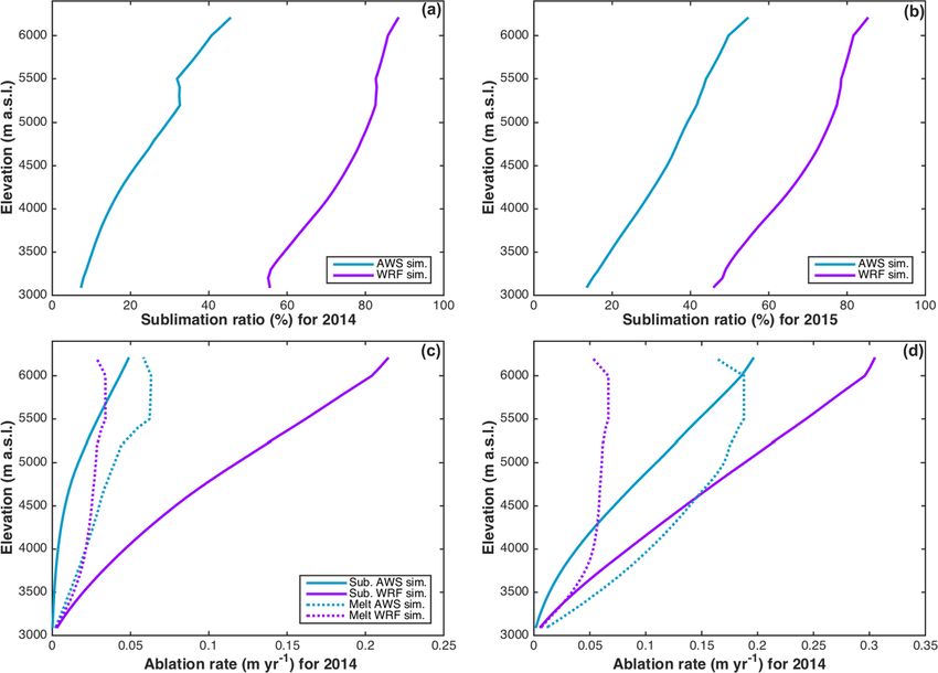
M. Réveillet et al.: Impact of forcing on sublimation simulations                                                            149

   The catchment covers an area of 513 km2 and elevations         likely to be much greater than these. More details regarding
range from 3150 to 6200 m a.s.l. (Fig. 1b). At these ele-         available measurements and the time periods for which these
vations, only minimal vegetation in the form of shrubs is         are available are provided in Fig. 2. Tapado records are re-
observed, so we do not consider vegetation in this study.         ported in Fig. 3 as an example of the weather conditions in
The study area includes rock glaciers and glaciers. Tapado        this catchment.
Glacier is the largest of these with an area of 2.2 km2              Due to the complexity of precipitation measurement
(Fig. 1b). This catchment was selected since it is an impor-      (e.g., MacDonald and Pomeroy, 2007), datasets were post-
tant water resource in the Elqui Valley. Indeed it feeds wa-      processed. First, filters were applied to eliminate outliers
ter to the La Laguna reservoir (38.106 m3 capacity), which        (i.e., negative values and values larger than 30 mm h−1 ). Sec-
is part of the strategic irrigation system in the Elqui Val-      ond, satellite images (MODIS Aqua and MODIS Terra) were
ley. Nevertheless the precipitation amount is very low. The       used to remove recorded precipitation events on sunny days,
mean annual precipitation measured at La Laguna station is        which were probably due to wind transport. These precipita-
200 mm a−1 and precipitation events are episodic with fewer       tion events were only removed if five cloud-free images were
than 10 events per year. In this region, most of these events     available (i.e., the two for the day: one the afternoon before
(90 %) occur during the winter period (Fig. S1, Rabatel et al.,   and one the next morning). In total, three precipitation events
2011) as snowfall. This seasonal difference is mainly due to      lower than 2 mm w.e. were removed with this method.
differences in the position and intensity of a high-pressure         At Tapado, measurements are recorded at two Geonor
cell in the eastern Pacific Ocean. During the summertime the      weighing precipitation gauges, of which one is shielded (alter
high-pressure cell limits advection, while during the winter it   shield) and one is unshielded. After being filtered, the cumu-
moves further north, allowing the moisture-laden depressions      lative difference at the two gauges was 9.1 mm for 2014 (i.e.,
to reach the study site (Garreaud et al., 2011). Seasonal pre-    10 %; 97.1 mm for unshielded gauge 1 and 106.2 mm for
cipitation variability and frequency are also complicated by      shielded gauge 2) and 5.4 mm for 2015 (i.e., 1 %; 457.5 mm
individual storm trajectories (e.g., Sinclair and MacDonell,      for gauge 1 and 462.9 mm for gauge 2) with a maximum
2016), which can cause large differences in relative precipi-     hourly difference of 1.1 mm; however the relative bias be-
tation distribution across the catchment, a phenomenon also       tween the sensors is neither constant nor unidirectional. As
described in central Chile (Burger et al., 2019).                 the difference between the two sensors was relatively small,
                                                                  the mean of the two datasets was used as the reference pre-
2.2     Data                                                      cipitation value, and a maximum uncertainty of 10 % was
                                                                  estimated.
2.2.1    Digital elevation model
                                                                  (b) WRF model outputs
The digital elevation model (DEM) used in this study was
derived from the CGIAR hole-filled 3 arcsec SRTM DEM re-
                                                                  The Weather Research and Forecasting (WRF) model was
sampled to 100 m resolution by the cubic method. The 100 m
                                                                  used to force SnowModel. WRF is usually used to predict
resolution was chosen to facilitate alignment of the model
                                                                  weather for atmospheric research and operational weather
grid with the 500 m resolution MODIS products (see below).
                                                                  forecasting. Using reanalysis data as boundary conditions,
2.2.2    Meteorological data                                      this model is able to provide hourly meteorological data such
                                                                  as air temperature, relative humidity, incoming radiation,
(a) Automatic weather station measurements                        wind speed and direction, atmospheric pressure, and precip-
                                                                  itation. In this study WRF was forced by 6-hourly data from
Meteorological data from nine Automatic Weather Stations          the National Centers for Environmental Prediction (NCEP)
(AWSs) are available in the catchment (Fig. 1b) over the          reanalysis data, at 1◦ grid resolution (Kalnay et al., 1996),
study period 2014–2015. La Laguna, Tapado and Paso del            as well as daily surface temperature of the ocean at 0.083◦
Agua Negra AWSs are scientific-grade permanent stations           of resolution. The WRF model has been run using the model
maintained by CEAZA (http://www.ceazamet.cl, last access:         version 3.7.1 (Skamarock and Klemp, 2008), with default pa-
December 2019) with hourly measurements. In addition, five        rameterizations (this choice is discussed in Sect. 5.1). The
HOBO ® weather stations (Colorado Bajo, La Gloria, Llano          model has been run over a time period covering the entire
de Las Liebres, Colorado Alto and Vega Tapado) were in-           study period (from April 2013 to April 2016). The model out-
stalled in March 2014 and set to record meteorological data       puts are at 2 m above the surface (note that wind output was
every 30 min. The Tapado Cubierto station was installed in        logarithmically scaled from 10 to 2 m height) and are avail-
2013 on the debris-covered part of the glacier and provides       able at 22 km resolution over Chile, 7 km resolution at the
measurements at hourly intervals. Although the lower accu-        regional scale and 3 km resolution over the La Laguna catch-
racy of HOBO weather sensors compared to the permanent            ment (Fig. 1). The hourly 3 km outputs (air temperature, T ;
stations represents a source of errors in the forcing data, er-   relative humidity, RH; wind speed, WS, and wind direction;
rors resulting from the spatial interpolation of forcings are     precipitation, P , shortwave radiation, SW; longwave radia-

www.the-cryosphere.net/14/147/2020/                                                       The Cryosphere, 14, 147–163, 2020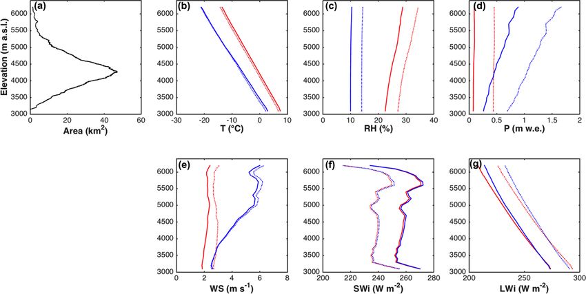
150                                                          M. Réveillet et al.: Impact of forcing on sublimation simulations

Figure 2. Date of available measurements from the nine AWSs used to calibrate and validate the model. T is the air temperature, RH
the relative humidity, SWi and LWi the incoming shortwave and longwave radiation, respectively, WS the wind speed, Pa the atmospheric
pressure, and SD the snow depth.

tion, LW; atmospheric pressure, Pa) over the catchment rep-          3     Method
resent the virtual stations that have been used in this study.
                                                                     3.1    SnowModel description
2.2.3   Local snow depth data

In 2014, three AWSs provided snow depth measurements at              The physically based model SnowModel (Liston and El-
an hourly time step (Vega Tapado, Tapado and Tapado Cu-              der, 2006b) was used to simulate the snow depth evolution
bierto; Fig. 2). Over the 2015 winter, snow depth measure-           over the entire catchment. SnowModel has already shown
ments were available at five stations (La Gloria, Colorado           acceptable performance in the challenging context of semi-
Alto, Tapado, La Laguna and Tapado Cubierto). The snow               arid mountains, including the Andes (Gascoin et al. 2013,
depths were measured with ultrasonic sensors and require             Mernild et al. 2017) and the High Atlas (Baba et al., 2018a,
post-treatment because they are particularly prone to mea-           b) mountains. It is a spatially distributed snowpack evolu-
surement errors and typically produce a noisy signal (Lehn-          tion modeling system composed of four submodels briefly
ing et al., 2002). Therefore, the control procedure described        described below.
in Lehning et al. (2002) was applied to clean the signal and in         MicroMet is a physically based meteorological distribu-
particular to eliminate spikes, check for outliers and physical      tion model developed specifically to produce high-resolution,
limits.                                                              spatially distributed atmospheric forcing data. This model re-
                                                                     quires precipitation, wind speed and direction, temperature,
2.2.4   MODIS snow products                                          and humidity as input data, generally measured at weather
                                                                     stations. For the incoming solar and longwave radiation and
MOD10A2 (Terra) and MYD10A2 (Aqua) snow products                     surface pressure, MicroMet can either compute these fields
version 5 were downloaded from the National Snow and Ice             from other meteorological variables or create them from ob-
Data Center (Hall et al., 2006; Hall and Riggs, 2007) for            servations through a data assimilation procedure (Liston and
the period 1 January 2014–1 January 2016. The binary snow            Elder, 2006a). MicroMet includes a preprocessor component
products were projected on a 500 m resolution grid in the            that first analyzes meteorological data to identify and correct
same coordinate system as the DEM. Missing values, mainly            potential deficiencies (e.g., values out of the ranges given in
due to cloud obstruction, were interpolated using the algo-          the subroutine). It then fills in any missing data segments
rithm of Gascoin et al. (2015).                                      with realistic values. The atmospheric fields are distributed
                                                                     using a combination of lapse rates and spatial interpolation
                                                                     using the Barnes objective analysis scheme (Barnes, 1964).

The Cryosphere, 14, 147–163, 2020                                                          www.the-cryosphere.net/14/147/2020/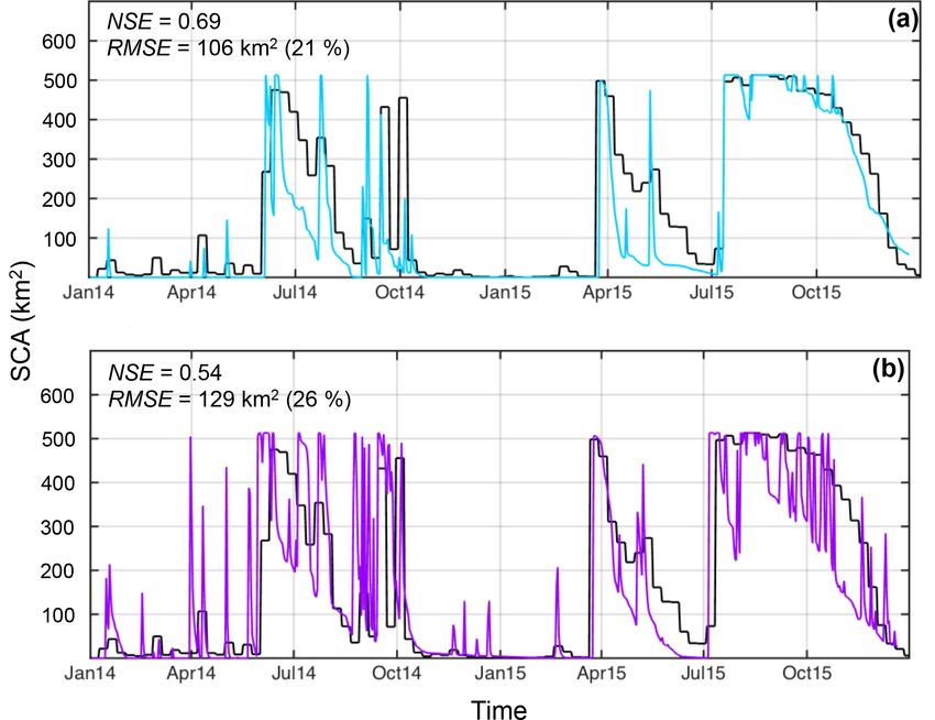
M. Réveillet et al.: Impact of forcing on sublimation simulations                                                                151

                                                                         SnowTrans-3D (Liston and Sturm, 1998; Liston et al.,
                                                                      2007) is a three-dimensional model that simulates snow
                                                                      depth evolution (deposition and erosion) resulting from
                                                                      windblown snow based on a mass balance equation that de-
                                                                      scribes the temporal variation in snow depth at each grid cell
                                                                      within the simulation domain.

                                                                      3.2     Model setup

                                                                      3.2.1    Spatialized meteorological forcing

                                                                      Spatial interpolation using the Barnes scheme was used to
                                                                      distribute the nine AWS measurements of T , RH, LWi, SWi
                                                                      and pressure over the model domain. As relative humidity
                                                                      is a nonlinear function of elevation, the relatively linear dew
                                                                      point temperature is used for the elevation adjustment. For
                                                                      more details refer to Liston and Elder (2006a). In this study
                                                                      the MicroMet subroutine has been run with the default set-
                                                                      ting for the Southern Hemisphere, for air temperature and
                                                                      dew point temperature monthly lapse rates (Liston and El-
                                                                      der, 2006b). Monthly lapse rates computed from the avail-
                                                                      able measurements are dependent on the year considered. As
                                                                      the mean is close to the default settings, it has been cho-
                                                                      sen to conserve these values. Radiation values for LWi and
                                                                      SWi are assimilated and specified using the default param-
                                                                      eterization (Liston and Elder, 2006a). The model has been
                                                                      run on the SRTM DEM and as a result, hourly meteorolog-
                                                                      ical data over a 100 m grid resolution are available for the
                                                                      entire study period. Precipitation was interpolated similarly
                                                                      but without considering a lapse rate, as the comparison be-
                                                                      tween the available measurements did not reveal consistent
                                                                      elevation gradients. Wind data and direction were first inter-
                                                                      polated using linear lapse rates and then each gridded value
                                                                      was corrected considering topographic slope and curvature
Figure 3. Example of meteorological conditions of the study area.     relationships (Liston and Elder, 2006b).
Daily air temperature (T ), relative humidity (RH), incoming short-      The 3 km WRF outputs (Sect. 2.2.1) were used as inputs
wave (SWi) and longwave (LWi) radiation, air pressure (Pa), precip-   for MicroMet, which considers that each WRF cell corre-
itation (P ), snow depth (SD), and hourly wind speed and direction    sponds to a virtual weather station located in the center of
(wind roses) measured at the Tapado AWS from 1 January 2014 to
                                                                      the WRF cell, following Mernild et al. (2017) and Baba et
31 December 2015. Note that SD measurements are available until
                                                                      al. (2018a). MicroMet adjusts the elevation bias to the DEM
1 August 2015.
                                                                      at the corresponding coordinate and downscales the data to a
                                                                      100 m grid.
   EnBal performs standard surface energy balance calcu-
                                                                      3.2.2    Albedo calibration
lations (Liston, 1995; Liston et al., 1999). This component
simulates surface temperatures and energy fluxes in response          The snow albedo evolution is computed as a function of the
to observed or modeled near-surface atmospheric conditions            snow density and air temperature (more details in Liston and
provided by MicroMet. Surface latent and sensible heat flux           Hall, 1995; Liston and Elder, 2006b). Minimum and maxi-
and snowmelt calculations are made using a surface energy             mum values have been adjusted based on measurements. The
balance model.                                                        minimum snow albedo (i.e., the soil) is fixed at 0.2 and is
   SnowPack is a single or multilayer (max. six layers), snow-        quite homogeneous in this basin, as there is almost no vegeta-
pack evolution and runoff or retention model that describes           tion. The minimum and maximum snow albedo (correspond-
snowpack changes in response to precipitation and melt                ing to old and fresh snow, respectively) are respectively fixed
fluxes defined by MicroMet and EnBal (Liston and Hall,                to 0.6 and 0.9 in agreement with all the measurements per-
1995; Liston and Elder, 2006b).                                       formed at the AWSs (Fig. 2).

www.the-cryosphere.net/14/147/2020/                                                           The Cryosphere, 14, 147–163, 2020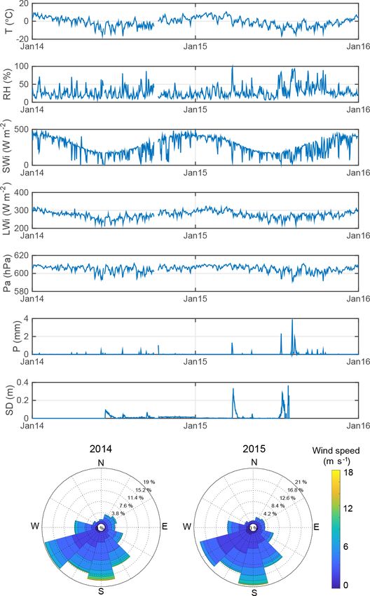
152                                                           M. Réveillet et al.: Impact of forcing on sublimation simulations

3.2.3    Turbulent flux calibration                                  Pr(e) represents the hypothetical probability of chance agree-
                                                                     ment. Complete agreement is defined when k = 1. The root-
As the model is using a bulk approach to simulate the tur-           mean-square error (RMSE) was also calculated.
bulent fluxes, the turbulent latent and sensible heat fluxes            Second, the model performance was evaluated over the en-
(respectively LE and H ) are parameterized using an effec-           tire catchment, by comparing the simulated snow cover ex-
tive surface roughness length z0 (Liston, 1995; Liston et al.,       tent and duration to that observed by the satellite images (de-
1999). Note that this roughness length z0 is considered an ef-       scribed in Sect. 2.2.2). The model performance was evalu-
fective value used in the model to represent the aerodynamic         ated by computing the Nash–Sutcliffe efficiency coefficient
(zm ), temperature (zt ) and humidity (zq ) roughness values.        (NSE; Nash and Sutcliffe, 1970) between simulations and
As no measurements from the study period are available to            observations and the RMSE.
calibrate and validate this value, it was initially fixed at 1 mm       After validating the model, the sublimation ratio and sub-
(Gromke et al., 2011; MacDonell et al., 2013a), and a subse-         limation and melt rates were computed over the catchment
quent sensitivity test was undertaken. Note that the surface         for the two years. The sublimation rate corresponds to the
temperature is solved iteratively by closing the energy bal-         mass sublimated per unit of time and does not include evap-
ance (Liston and Elder, 2006b). In addition, under stable at-        oration from meltwater. The sublimation ratio is defined as
mospheric conditions, turbulent fluxes are modified based on         a percentage and equal to the sublimation divided by the to-
a Richardson number correction (Liston and Hall, 1995).              tal ablation (i.e., sublimation plus melt rates). The melt rate
                                                                     corresponds to meltwater that runs off from the snowpack.
3.2.4    Wind transport parameterization                             Whilst the model calculates refreezing, the final melt rate
                                                                     described here does not include snowmelt that refreezes in
The model considers the wind transport (saltation, turbulent
                                                                     the snowpack. Note that ablation and energy balance terms
suspension) after snow deposition, sublimation of blowing
                                                                     are only computed over snow surfaces. This means that an-
and drifting snow, and erosion and deposition after snowfall,
                                                                     nual and monthly means are only computed at grid cells with
depending on the topography (Liston and Sturm, 1998). The
                                                                     snow.
topographic influence on wind transport has been set, fol-
lowing Gascoin et al. (2013). The curvature allows consider-
                                                                     3.4     Comparison with MODIS
ation of the typical redistribution length scale. Based on the
DEM, it was estimated to be 500 m, i.e., approximately one-
                                                                     The snow cover area (SCA) and the snow cover dura-
half the wavelength of the topographic features within the
                                                                     tion (SCD) over the entire catchment were compared to
domain (Liston et al., 2007). The model considers different
                                                                     the MODIS product. A threshold of 0.003 m w.e. was used
weights for slope and curvature values. We have chosen 0.58
                                                                     to convert the simulated snow water equivalent (SWE) into
and 0.42, respectively, following Gascoin et al. (2013).
                                                                     snow presence or absence for each grid cell (within the same
3.3     Simulations                                                  range as Gascoin et al., 2015). Since the MODIS SCA prod-
                                                                     uct corresponds to the maximum visible extent over a period
Two types of simulations have been performed over the entire         of 8 d, we also computed the maximum SCA over the same
catchment for the period 1 January 2014–1 January 2016 on a          8 d period from the simulated SCA for comparison.
100 m resolution DEM. The first simulation was forced with
input from the nine automatic weather station measurements
(referred to as AWS forcing), whereas the second simulation          4     Results
was forced with the WRF data (referred to as WRF forcing).
   After indicating the differences observed for these two           4.1     Meteorological forcing comparison
forcing sets, the model is primarily validated at local points.
Results for the two simulations were first compared to lo-           4.1.1    AWS 2014 vs. 2015
cal snow depth measurements at each AWS (described in
Sect. 2.2.1). The performance was evaluated using a kappa            According to the AWS measurements, January–July 2015
statistic coefficient (Cohen, 1960) denoted k to measure the         was warmer than January–July 2014. Conversely, ob-
agreement between the simulation and the observation, con-           servations indicate lower temperatures for August–
sidering the percentage of time with and without snow. The           December 2015 than for August–December 2014 (daily
calculation of k is here performed according to the following        mean difference of −2.6 ◦ C). Relative humidity was higher
formula:                                                             for 2015 compared to 2014 (daily mean difference of 11 %)
      Pr (a) − Pr(e)                                                 whereas SWi was lower (mean difference of −18 W m−2 ,
k=                   ,                                       (1)     i.e., 6 % of the mean SWi), with larger differences in
        1 − Pr(e)
                                                                     July–December (daily mean difference of −32 W m−2 , i.e.,
where Pr(a) represents the actual observed agreement (i.e.,          12 % of the daily mean SWi), and LWi was higher (daily
snow or no snow for both simulation and observation), and            mean difference of 20 W m−2 , i.e., 7 % of the daily mean

The Cryosphere, 14, 147–163, 2020                                                         www.the-cryosphere.net/14/147/2020/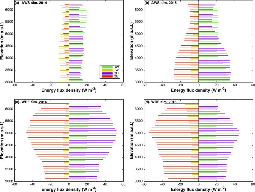
M. Réveillet et al.: Impact of forcing on sublimation simulations                                                                  153

Figure 4. (a) Area–elevation distribution of the La Laguna catchment. (b–g) MicroMet outputs at the catchment scale forced by the AWS
(red) and the WRF (blue) for 2014 (lines) and 2015 (dashed lines).

LWi). This decrease in SWi and increase in LWi can be
explained by a higher degree of cloud cover in 2015.

4.1.2    MicroMet output comparison: AWS vs. WRF

Figure 4 shows MicroMet outputs forced by WRF and AWS.
Colder air temperatures are observed for the WRF forcing
(4.5 to 7.5 ◦ C depending on the year and the elevation), as
well as lower RH (between 13 % and 24 %) and higher pre-
cipitation (annual cumulative difference larger than 1 m w.e.
and a difference ranging between a factor of 1.6 and 3.4 de-
pending on the elevation; Fig. 4d). The SWi and LWi remain
very similar. The wind speed outputs differ (Fig. 4e), espe-
cially above 4500 m a.s.l. where differences reach a maxi-
mum of 4 m s−1 . Details and statistical information about the
comparison at each AWS location are available in Table S1
(in the Supplement). Note that here the comparison between
the AWS measurements and the closest WRF grid point is
not presented due to the significant vertical offset between
the two points (Table S1). Despite these differences between
AWS and WRF, both forcings were used as inputs in order to
quantify the impact of the forcing choice on the sublimation
estimation in this study.

4.2     Snow depth and snow cover comparison

4.2.1    Comparison with local snow depth measurements               Figure 5. Simulated (cyan and purple) vs. observed (red) snow
                                                                     depth at six automatic weather stations. Cyan lines (a–f) represent
Simulated snow depths using the AWS forcing (Fig. 5a–f)              simulations performed using AWS meteorological forcing. Purple
are in good agreement with measured snow depth values                lines (g–m) correspond to simulations performed using WRF mete-
(mean k = 0.14 and mean RMSE = 0.15 m, corresponding                 orological forcing. Grey shaded areas indicate the period of avail-
to 36 % of the maximum mean snow depth). Note that the               able measurements.

www.the-cryosphere.net/14/147/2020/                                                           The Cryosphere, 14, 147–163, 2020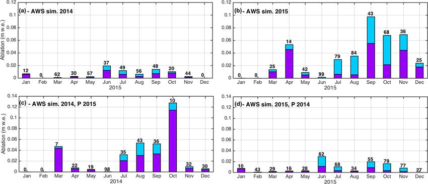
154                                                         M. Réveillet et al.: Impact of forcing on sublimation simulations

largest RMSE corresponds to 63 % of the maximum snow
depth. Comparisons have been performed at individual sta-
tions for 2014 and 2015, and we observe better performances
across all stations (i.e., higher k and lower RMSE) for 2015
(Fig. 5d–f) than for 2014 (Fig. 5a–c). For 2014 the highest
k and lower RMSEs are observed at Tapado AWS, as pre-
cipitation measurements were available at this site, but per-
formances are much lower at the two other sites where pre-
cipitation was interpolated. Interpolation results in overesti-
mation of the simulated snow depth during 2015, probably
due to an overestimation of the precipitation for the large
event on 21 June 2015 (Fig. 3) caused by large differences in
measured precipitation at the La Laguna and Tapado AWSs
in particular. Nevertheless, the start and the end dates of the
snow season are in good agreement with observations (max-
imum difference of 3 d observed at La Gloria site). Note that
this comparison probably overestimates the accuracy as snow
                                                                   Figure 6. Snow cover area evolutions over the 2014–2015 period,
depths are compared at the exact location of meteorological        from MODIS images (black lines), and simulations using (a) AWS
forcing. Larger uncertainties are expected at the interpolated     forcing (blue line) and (b) WRF forcing (purple line).
locations.
   Simulations performed with the WRF forcing indicate
lower performances in simulating snow depth evolution at           4.2.2   Snow cover comparison with satellite images
the AWS (Fig. 5g–m; mean k = 0.12, and mean RMSE =
0.20 m, corresponding to 39 % of the maximum mean snow             4.2.3   (a) Snow cover area
depth, and the largest RMSE corresponds to 76 % of the max-
imum snow depth). The results indicate an overestimation of        The simulated snow cover area (SCA), forced by the
the simulated snow depth compared to the observations. In          AWS forcing, is in good agreement with observations from
addition, for 2014, the timing of the start and the end of the     MODIS products (Fig. 6a) with, in particular, a good sim-
snow season does not fit well with observations (and explain       ulation of the timing of precipitation events. Best fits are
the low k values). In 2015, the first day of snow is generally     observed for the winter and spring 2015 (i.e., from July to
in good agreement with observations (maximum difference            December), with higher calculated correlations (NSESCA =
of 5 d observed at La Laguna).                                     0.94, RMSESCA = 41.6 km2 , i.e., 8.3 %). Regarding the ab-
   While AWS forcing yields a better performance overall, in       lation, in June 2014 and April–May 2015, the simulated SCA
both cases better correspondence is obtained for 2015. This        decreases faster than the observed SCA, which can be due to
could possibly be explained by the dry conditions in 2014,         an overestimation of melt and/or sublimation or an underes-
which would have resulted in precipitation having a higher         timation of accumulation.
spatial variability. The low snow amounts in 2014 created             When using the WRF forcing, the agreement between
localized snow patches, which are complex to represent in          SCA and MODIS is lower than with the AWS forcing
models.                                                            (Fig. 6b). The timing of snowfall events is not always in good
   These results underline the complexity of modeling the          agreement with the observations due to missing events (e.g.,
spatial variability of snow depth (SD), even when snow trans-      March 2015), a timing bias of a few days (e.g., March 2014)
port is implemented. Results show an overall similarity of the     and/or additional events (during both 2014 and 2015 win-
simulated SD between some stations (e.g., Vega Tapado, Col-        ter). The simulated SCA evolution over winter and spring
orado Alto and La Gloria), while measurements indicate that        of 2015 shows strong variation over the entire catchment,
SD is much more variable in reality. Note that the windy con-      which is not observed in the MODIS record. Here again, for
ditions on the local depression at Vega Tapado are very local      both forcing datasets, better performances are observed for
(i.e., few meters) and make the simulation at this site where      2015 (NSEAWS = 0.79, RMSEAWS = 93.2 km2 , i.e., 19 %
the measured SD is larger than the surrounded area and not         of the total area; NSEWRF = 0.61, RMSEWRF = 125 km2
representative of the 100 m grid cell complicated.                 (25 %)) than for 2014 (NSEAWS = 0.41, RMSEAWS =
                                                                   117 km2 (23 %); NSEWRF = 0.23, RMSEWRF = 133 km2
                                                                   (27 %)).

The Cryosphere, 14, 147–163, 2020                                                       www.the-cryosphere.net/14/147/2020/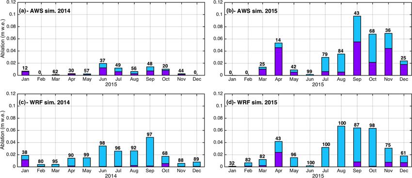
M. Réveillet et al.: Impact of forcing on sublimation simulations                                                             155

(b) Snow cover duration over the catchment                         explaining the larger values of the sublimation ratio at high
                                                                   elevations.
The simulated snow cover duration (SCD) was also com-
pared to the observed duration (from MODIS) by elevation           (b) Energy fluxes
band (Figs. 7, S2). For each 200 m elevation band, the total
number of snow-covered days for each grid cell was com-            Figure 9 shows the distribution of energy fluxes with eleva-
puted and then averaged for each band. For 2014, better per-       tion to aid the interpretation of the relationship between ele-
formances were obtained for the AWS forcing than for the           vation and sublimation for both forcings. Both LW and SW
WRF forcing (Fig. 7). For 2015, while better performances          show little variability between elevation bands for the AWS
were also obtained for the AWS forcing, the improvement            forcing. LW also does not change strongly between years.
using this forcing was minor.                                      The SW and turbulent fluxes, however, show a strong vari-
   Results based on AWS forcing are in good agreement              ability between 2014 and 2015. For 2015 the modeled turbu-
with observations at low elevations (i.e., below 4600 m a.s.l.;    lent fluxes (mainly the latent heat flux, QE) are higher, es-
Fig. 7) but show an overestimation of the SCD at high eleva-       pecially at lower elevations, resulting in higher sublimation
tion (absolute mean difference of 30 and 27 d for 2014 and         ratios (Fig. 8a, b., Sect. 4.3.1a). The WRF simulations, on the
2015, respectively).                                               other hand, do not show this interannual difference in energy
   When using WRF forcing, SCD is overestimated for the            fluxes. Comparison of the AWS and WRF simulations, how-
entire catchment in 2014 (absolute mean difference of 67 d).       ever, show higher turbulent fluxes for WRF forcing, which is
In 2015, simulations indicate an overestimation of the SCD         in agreement with the higher sublimation rate and ratio men-
at low elevations (i.e., below 4500 m a.s.l.) and a small under-   tioned above.
estimation at higher elevations (absolute mean error of 34 d
for 2015).                                                         4.3.2    Monthly evolution

4.3     Ablation and energy balance fluxes                         Analysis of the monthly sublimation ratios and rate shows
                                                                   a strong seasonal variability in sublimation (Fig. 10). In-
The forcing strongly impacts the simulated sublimation ratio.      dependently of the forcing chosen, larger sublimation rates
The annual means computed over the entire catchment (only          are found in June and September for 2014 and in August,
considering snow grid-cells) for the AWS forcing were 42 %         September and October for 2015, corresponding to the warm
and 49 % for 2014 and 2015, respectively, whereas 86 % and         parts of the snow season.
80 % were obtained for WRF forcing. The mean daily rate               Figure 11 indicates that turbulent fluxes (QE and QH) have
is 0.6 and 3.6 w.e. d−1 for 2014 and 2015, respectively, when      the greatest impact on sublimation in all cases, except for the
the model is forced with the AWS forcing. Values are larger        2014 AWS simulation. Net SW is also an important factor,
and reach 3.1 mm w.e. d−1 and 4.1 mm w.e. d−1 for 2014 and         and relatively similar for all the simulations. For the annual
2015 when simulations are performed with the WRF forcing.          mean, net SW is 18 and 22 W m−2 for 2014 and 2015 for
                                                                   the AWS forcing and 24 and 23 W m−2 for the WRF forcing,
4.3.1    Mean annual elevation gradients                           respectively. The contribution of net LW on the other hand is
                                                                   low for all simulations (annual mean of −7 and −6 W m−2
(a) Ablation                                                       for AWS and WRF simulations, respectively). Note that these
                                                                   losses are small in comparison to midlatitude sites (e.g., −25
The annual sublimation ratio is variable in space and in-          to −20 W m−2 according to the study by Giesen et al., 2009)
creases with elevation for both years and both forcings            because of the very dry conditions of the atmosphere and the
(Fig. 8a, b). Comparison between the two forcings shows            cold surface temperature of the snow surfaces.
larger discrepancies below 5300 m a.s.l. (50 % of differences
for 2014 and 30 % for 2015). Note that larger differences
were observed for 2014 related to larger differences in snow       5     Discussion
cover and snow duration between forcings.
   Melt predominates at all elevations when using the AWS          5.1     AWS vs. WRF forcing
forcing (Fig. 8c, d), except above 6000 m a.s.l. in 2015.
Melt and sublimation rates increase with elevation until           Results presented in this study highlight the importance of
5300 m a.s.l. Above this elevation the melt rate first stagnates   forcing when modeling snow depth, snow cover and subli-
and subsequently decreases. This increase in sublimation rate      mation. Differences in model outputs are largely due to dif-
and decrease in melt at high elevations explains the increase      ferences in temperature and precipitation inputs.
in sublimation ratio with elevation observed in Fig. 8a, b.
   For the WRF forcing, sublimation rates are larger than
the melt rates at all elevations. Melt is relatively constant
above 3800 m a.s.l., whereas the sublimation ratio increases,

www.the-cryosphere.net/14/147/2020/                                                        The Cryosphere, 14, 147–163, 2020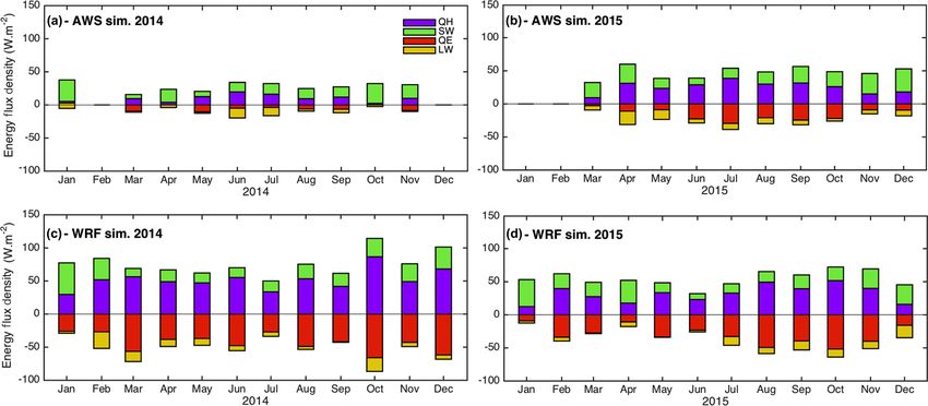
156                                                          M. Réveillet et al.: Impact of forcing on sublimation simulations

Figure 7. Snow cover duration per 200 m elevation band, from MODIS images (black), AWS forcing (blue) and WRF forcing (purple) for
(a) 2014 and (b) 2015.

5.1.1   Air temperature and precipitation                           adjust WRF data with measurements. More studies compar-
                                                                    ing WRF output to AWS among other datasets are required
The cold bias in air temperature from WRF simulations, us-          to determine a realistic correction method.
ing the combination NCEP–WRF, is often observed and well
documented (e.g., Ruiz et al., 2010). It can be explained by        5.1.2   Consequences of the forcing used
the model parameterization complexity such as (i) the initial
or lateral conditions, especially for the land surface surface      Biases between the two forcing datasets cause significant dif-
temperature (Cheng and Steenburgh, 2005) or soil thermal            ferences in the energy and associated mass balances during
conductivity (Massey et al., 2014); (ii) the parameterization       both study years. In 2014 there are lower RH and P biases
of the planetary boundary layer scheme (Reeves et al., 2011);       (Fig. 4c, d), but larger air T differences, especially at high
or (iii) the radiation parameterization scheme as it has been       elevations (Fig. 4b). Wind speed is on average higher in the
observed for other models (e.g., Müller and Scherer, 2005).         WRF forcing, whereas biases in incoming LW and SWi and
However, the exact source of this bias remains difficult to         air pressure are low for both years (results not shown).
identify (e.g., Reeve et al., 2011). In this study, the default        The larger RH bias in 2015 indicates an overestimation
parameterization has been used, but works are in progress           of the dryness for this year (compared to 2014) and would
regarding the evaluation of the most appropriate calibration        lead to larger differences in sublimation rate for 2015 than
over this area, using direct observations.                          for 2014, which is the opposite of the results observed. Like-
   Otherwise, precipitation is known to be overestimated us-        wise, the larger overestimation of precipitation amount ob-
ing the WRF model, particularly in the Andes (e.g., Mourre          served in 2015 (Fig. 4d) does not explain the larger difference
et al., 2016). One possible explanation is that biases can exist    in sublimation, as a deeper snow depth should result in more
in the reanalysis data, in particular at high elevations, where     persistent snow cover during the warm period and hence a
observations are often scarce. Precipitation overestimation         lower sublimation ratio related to larger melt rate. Therefore,
might also be related to the parameterization used for the          although the relationship between temperature and sublima-
model, which may not be the most appropriate for the An-            tion rate is complex and not necessarily direct, in this case,
des; further work is needed to determine the most appropri-         the colder temperature is the most probable explanation for at
ate ones. Outputs may also be inaccurate due to the relatively      least part of the larger difference in sublimation rate observed
low-resolution DEM used (100 m).                                    at high elevation.
   Precipitation measurements using rain gauges can be bi-             Lower temperature and relative humidity values from
ased towards an underestimation due to an undercatch, es-           WRF outputs compared to AWS measurements can explain,
pecially for snowfall because of the influence of wind (e.g.,       in part, the larger simulated sublimation ratio found with this
MacDonald and Pomeroy, 2007; Wolff et al., 2015). This              forcing (Figs. 8a, b and 10). The relatively high amounts of
gauge undercatch uncertainty (see Sect. 5.4.1) could increase       precipitation simulated by the WRF outputs, and resulting
the difference between the precipitation simulated by WRF           snow cover overestimation, may also play a role. Differences
and that measured at the AWSs. In addition, questions arise         in the sublimation ratio when using the AWS and WRF forc-
regarding the representativity of point measurements com-           ing are quite similar for the two years (mean annual differ-
pared to the grid cell considered in the model.                     ence of 42 % and 36 % for 2014 and 2015, respectively), al-
   The spatiotemporal variability observed in the difference        though the difference between the melt rate and sublimation
between AWS and WRF precipitation data highlights that it           rate depends on the year (Figs. 8c, d) and corresponding en-
would be inappropriate to use a constant correction factor to       ergy balance.

The Cryosphere, 14, 147–163, 2020                                                        www.the-cryosphere.net/14/147/2020/
M. Réveillet et al.: Impact of forcing on sublimation simulations 157 Figure 8. Simulated annual sublimation ratio against elevation band using AWS (blue) and WRF (purple) forcing for 2014 (a) and 2015 (b). Simulated annual average total ablation (sublimation and melt) against the elevation using AWS and WRF forcing for 2014 (c) and 2015 (d). Figure 9. Annual mean of main modeled energy fluxes (computed over snow surfaces only) for each 200 m elevation band using AWS (a, b) and WRF (c, d) forcing for 2014 (a, c) and 2015 (b, d). SW is net shortwave radiation, LW is net longwave radiation, QE is the latent heat flux and QH is the sensible heat flux. www.the-cryosphere.net/14/147/2020/ The Cryosphere, 14, 147–163, 2020
158                                                         M. Réveillet et al.: Impact of forcing on sublimation simulations

Figure 10. Stacked simulated melt (purple) and sublimation (blue) per month using AWS forcing (a, b) and WRF forcing (c, d). Black
numbers indicate the monthly sublimation ratio in percent.

Figure 11. Monthly average of the main modeled energy fluxes for the entire catchment, over snow surfaces only. SW is net shortwave
radiation, LW is net longwave radiation, QE is the latent heat flux and QH is the sensible heat flux.

   In 2014 the turbulent fluxes are dominant for the WRF               The large variation in the SCA resulting from the WRF-
forcing but not for the AWS forcing (Fig. 9a, c). This can          driven model results (Fig. 5) is likely related to the higher
be partially explained by the larger SCA simulated by WRF           frequency of relatively small precipitation events modeled
forcing with snow cover in the entire catchment while the           by WRF than are recorded by the AWS. These small events
AWS forcing only results in snow at higher elevations. Ad-          cover the catchment with a relatively thin layer of fresh snow,
ditionally, WRF forcing indicates colder, drier and windier         which sublimates relatively quickly, causing the SWE to de-
conditions than the AWS forcing (Fig. 4). Lower RH and              crease to < 3 mm w.e. at lower elevations, causing high vari-
higher wind speed will directly increase the latent heat flux,      ability in modeled SCA.
and potentially sublimation ratio, depending on surface tem-           The SCD also has a significant influence on sublimation.
perature (see Fig. S3 for surface temperature comparison).          For 2014, the differences in SCD between the two forcings

The Cryosphere, 14, 147–163, 2020                                                        www.the-cryosphere.net/14/147/2020/
M. Réveillet et al.: Impact of forcing on sublimation simulations                                                             159

were 100 d below 4500 m and close to 50 d above this eleva-        5.2.2   Impact of the precipitation amount
tion (Fig. 7a). Snow that persists until later in the year (aus-
tral spring and summer) results in an increased total melt rate
and can influence the sublimation ratio (especially in 2015,       Forcing the 2014 year with the wet precipitation input re-
Fig. 10). This is the only explanation for the larger melt frac-   duces the mean annual sublimation ratio by 12 % (Fig. 12a,
tion observed with AWS forcing compared to WRF forcing at          d), while forcing the 2015 year with the dry precipitation
low elevations, given the cold bias in WRF forcing (Figs. 8c       input increases the mean annual sublimation ratio by 3 %
and 4b). Since a larger SCD can be related to larger precip-       (Fig. 12b, d). In summary, a decreased annual mean subli-
itation amount, precipitation uncertainties likely play a sig-     mation ratio is observed when the precipitation is increased
nificant role in the sublimation estimation.                       (which likely increases the SD and SCD) and other factors
                                                                   are held constant. However the amplitude of the response
5.2     Comparison between dry and wet conditions                  differs between the two years. This is mainly due to differ-
                                                                   ences in the ablation rates (Fig. 12). For 2014, increasing the
5.2.1    Comparison between 2014 and 2015                          precipitation amount leads to a sublimation rate increase of
                                                                   0.8 mm w.e. d−1 while for 2015, decreasing the precipitation
Differences in sublimation ratio and rates between 2014 and
                                                                   amount decreases the rate by 2.8 mm w.e. d−1 . Despite these
2015 are related to both meteorological conditions related to
                                                                   annual differences, the maximum monthly sublimation rates
energy fluxes and snow cover duration. First, the similar an-
                                                                   are still observed for the same months, independent of the
nual mean sublimation ratio found for both years is likely due
                                                                   precipitation forcing used, with the exception of June and
to a compensation between the dry 2014 year (low precipita-
                                                                   August (Fig. 12). In June, snow covered the entire catchment
tion) associated with cold conditions in spring and summer
                                                                   in 2014 but not in 2015 (Fig. 6), related to a strong snow
and the wet 2015 year with longer snow duration and warmer
                                                                   event in June 2014 and no precipitation in June 2015. The
spring and summer (according to meteorological measure-
                                                                   opposite was observed for August. Changing the precipita-
ments made in the region). Both sublimation and melt rates
                                                                   tion forcing strongly impacts the SCA and therefore the snow
were larger overall during the wet 2015 year compared to the
                                                                   amount available for ablation and sublimation.
dry 2014 year. Thus the higher melting rates in 2015 com-
                                                                      Comparisons made for months with a maximum SCA (i.e.,
pensated for the enhanced sublimation rates and resulted in
                                                                   when the entire catchment is covered by snow and it per-
sublimation ratios comparable with 2014. The larger subli-
                                                                   sists over the entire month) allow the influence of SCD to be
mation rates observed in 2015 are related to higher RH and
                                                                   independently analyzed since the SCA remains constant. In
wind speed, but also higher precipitation, snow accumulation
                                                                   July, a month where maximum SCA was observed in both
and snow duration in 2015 compared to 2014. Results show
                                                                   years, sublimation differences of 27 and 57 mm w.e. m−1
particularly large sublimation rates over the long melt period
                                                                   were found between dry and wet precipitation inputs for
in 2015. This may be explained by the warmer conditions
                                                                   2014 and 2015, respectively. In 2015 the SD was thicker than
which induce a warmer snowpack, increasing the saturated
                                                                   in 2014 for both dry and wet inputs; thus the results indicate
vapor pressure at the snow surface and providing energy to
                                                                   an increased sublimation rate with thicker SD. The thicker
increase the sublimation rates (Herrero and Polo, 2016). Ac-
                                                                   SD also implies larger melt rates, such that the sublimation
cording to these results, the snow duration seems to modulate
                                                                   ratio decreases when increasing the precipitation in 2014 but
the annual average ablation ratio, such that a longer-lasting
                                                                   increases with increased precipitation in 2015, highlighting
snow cover extending further into the warm spring climate is
                                                                   the complexity of the influence of SD on the sublimation ra-
subjected to both enhanced sublimation and melt in response
                                                                   tio.
to an increase in incoming energy fluxes. Nevertheless, it re-
                                                                      Otherwise, differences in mean sublimation rates are much
mains difficult to disentangle the respective effects of mete-
                                                                   higher when changing the precipitation amount for the 2015
orological conditions and snow duration on sublimation. To
                                                                   meteorological forcing than for the 2014 meteorological
better evaluate these effects, the influence of the meteoro-
                                                                   forcing (i.e., 0.8 mm w.e. d−1 for 2014 vs. 2.8 mm w.e. d−1
logical forcing related to energy fluxes and the snow cover
                                                                   for 2015 as mentioned above). Sublimation rates are also
duration must be evaluated separately. For that purpose, we
                                                                   higher in 2015 compared to 2014, especially at the end
performed simulation experiments in which a common pre-
                                                                   of the snow season (i.e., from September to November;
cipitation input was used for both years. In the first experi-
                                                                   Figs. 12a, d). This holds true when considering wet condi-
ment the 2014 precipitation inputs (“dry input” with shorter
                                                                   tions (Fig. 12b, c). This highlights the significant influence
snow cover duration) were applied to both years, and then
                                                                   of meteorological conditions on sublimation. As mentioned
the 2015 precipitation was applied to both years (“wet input”
                                                                   in Sect. 5.2.1, 2015 experienced higher wind speeds and RH
with longer snow cover duration). All other meteorological
                                                                   and colder air temperatures. The contribution of turbulent
forcings were left unchanged.
                                                                   fluxes is higher in 2015 than 2014 (Fig. S4a, d), suggesting
                                                                   that wind speed has a greater influence on sublimation than
                                                                   RH.

www.the-cryosphere.net/14/147/2020/                                                        The Cryosphere, 14, 147–163, 2020
160 M. Réveillet et al.: Impact of forcing on sublimation simulations
Figure 12. Monthly simulated melt (purple) and sublimation (blue) using AWS forcing (a, b) and AWS forcing with (c) 2015 precipitation
(“wet forcing”) and (d) 2014 precipitation (“dry forcing”). Back numbers indicate the monthly sublimation ratio in percent.
5.3 Limits of the study snow cover using the AWS forcing are more realistic, both
at the local scale (comparison with AWS snow depth mea-
The main objective of this study was to investigate the impact surements) and over the entire catchment (comparison with
of forcing data on modeled mass and energy balance to ex- SCA and SCD from MODIS images). In addition, indepen-
plain sublimation ratios. Nevertheless, we recognize that un- dently of the forcing choice, the simulation of snow cover
certainties also exist depending on model calibration choices. is better for 2015 compared to 2014, mainly due to a larger
To discuss this point, four different parameters were tested sensitivity to the precipitation uncertainties during dry con-
to evaluate the uncertainties related to the calibration of ditions. This highlights the complexity in properly modeling
modeled parameters: roughness value, precipitation amounts the snow cover evolution for years with low precipitation.
(due to measurement uncertainties), topographic curvature There are also large differences in modeled sublimation ra-
length and slope versus curvature length (Fig. S5; Supple- tio depending on the forcing chosen. When using WRF forc-
ment Sect. S6). The results showed that the sublimation ra- ing the sublimation ratio is approximately twice that mod-
tio was most sensitive to roughness values and that differ- eled with the AWS forcing. This is partially due to the dif-
ences due to the other three variables were an order of magni- ferences in temperature and relative humidity between the
tude lower (for more details, please refer to the Supplement). two forcings, but mostly due to precipitation differences. For
The strong sensitivity to the roughness value and the absence example, when holding all model inputs constant except for
of measurements to validate the turbulent fluxes’ calibration precipitation, there are significant differences in the modeled
limits precise sublimation quantification for this area. sublimation, especially for 2014, which was a dry year. Oth-
erwise, the annual mean of the sublimation ratio over a catch-
ment is similar during the two years, but it increases with
6 Conclusion
elevation. This partly explains the larger sublimation values
In this study, the snow energy and mass balance have been reported in previous studies performed at high elevations in
simulated over La Laguna catchment located in the semi- the semiarid Andes of Chile (e.g., Gascoin et al., 2013; Ginot
arid Andes of Chile. Using the snowpack model SnowModel, et al., 2001; MacDonell et al., 2013a).
simulations were performed over two contrasting years (2014 Sublimation simulated in this study is associated with sev-
considered a dry year and 2015 considered a wet year), using eral sources of uncertainty related to the forcing chosen and
two distinct forcings (nine AWS located in the catchment and the model calibration. Regarding the calibration, the rough-
3 km resolution WRF model outputs). ness value is the key concern to properly simulate the tur-
Results indicate strong differences in simulated snow bulent fluxes, and results showed strong sensitivity to this
depth depending on the forcing chosen, mainly due to a cold value. Nevertheless, without measurements to properly cali-
bias in air temperature in WRF as well as an overestimation brate this value, it appears to be the main source of model cal-
of precipitation. As a result, performances in simulating the ibration uncertainty. Results presented here highlight precip-
The Cryosphere, 14, 147–163, 2020 www.the-cryosphere.net/14/147/2020/M. Réveillet et al.: Impact of forcing on sublimation simulations 161
itation as the main forcing uncertainty, due to measurement Financial support. Marion Réveillet and Shelley MacDonell were
errors and lack of spatial representation as precipitation data supported by CONICYT-Programa Regional R16A10003, and the
were only available for two stations. Precipitation uncertain- Coquimbo regional government FIC-R(2015) BIP 30403127-0.
ties directly impact snow on the ground and therefore indi- Christophe Kinnard was supported by a Coopération bilatérale –
rectly impact sublimation rates. Uncertainties in wind speed Québec-Chili Ministère des Relations Internationales et Franco-
phonie.
were likely the second source of error in sublimation re-
sults, which need to be better constrained in future studies.
Therefore, this study highlights that this uncertainty has a
Review statement. This paper was edited by Ross Brown and re-
strong impact on sublimation and further work is suggested viewed by Jonathan Conway and Kay Helfricht.
to (i) improve measurement uncertainties, (ii) increase the
number of sensors over the catchment, and (iii) incorporate
AWS measurements into the WRF model and use data as-
similation to improve model outputs. CEAZA is currently References
working on point (iii) to provide improved WRF outputs for
the semiarid Andes of Chile. This study has highlighted the Ayala, A., Pellicciotti, F., MacDonell, S., McPhee, J., and Bur-
lando, P.: Patterns of glacier ablation across North-Central
current difficulties in using standard WRF model outputs in
Chile: Identifying the limits of empirical melt models under
a semiarid Andean catchment. Moving forward, it would be sublimation-favorable conditions, Water Resour. Res., 53, 5601–
highly advantageous to improve WRF model performance in 5625, https://doi.org/10.1002/2016WR020126, 2017.
mountainous areas where high relief and difficult access of- Baba, M., Gascoin, S., and Hanich, L: Assimilation of Sentinel-
ten limit AWS distribution to valley floors, therein limiting 2 Data into a Snowpack Model in the High Atlas of Morocco,
the accuracy of interpolation techniques for terrain-sensitive Remote Sens., 10, 1982, https://doi.org/10.3390/rs10121982,
variables, such as precipitation and wind speed and direction. 2018a.
Baba, M., Gascoin, S., Jarlan, L., Simonneaux, V., and Hanich, L.:
Variations of the Snow Water Equivalent in the Ourika Catch-
Data availability. Part of the data used in this paper (automatic ment (Morocco) over 2000–2018 Using Downscaled MERRA-
weather station data) can be accessed at https://www.ceazamet.cl 2 Data, Water, 10, 1120, https://doi.org/10.3390/w10091120,
(CEAZA, 2020). Satellite images are available by contacting Si- 2018b.
mon Gascoin. Data were processed using the snowpack model Barnes, S. L.: A technique for maximizing details in numerical
SnowModel and this algorithm can be accessed by contacting the weather map analysis, J. Appl. Meteorol., 3, 396–409, 1964.
administrator, Glen E. Liston. For any other access to the data pre- Burger, F., Ayala, A., Farias, D., Shaw, T. E., MacDonell,
sented in this study, please contact the corresponding author. S., Brock, B., McPhee, J., and Pellicciotti, F.: Interannual
variability in glacier contribution to runoff from a high-
elevation Andean catchment: understanding the role of de-
Supplement. The supplement related to this article is available on- bris cover in glacier hydrology, Hydrol. Process., 33, 214–229,
line at: https://doi.org/10.5194/tc-14-147-2020-supplement. https://doi.org/10.1002/hyp.13354, 2019.
CEAZA: AWS data, available at: https://www.ceazamet.cl, last ac-
cess: 10 January 2020.
Cheng, W. Y. and Steenburgh, W. J.: Evaluation of surface sensi-
Author contributions. MR and SM designed the study. MR and
ble weather forecasts by the WRF and the Eta models over the
SG designed the modeling strategy. MR ran the numerical exper-
western United States, Weather Forecast., 20, 812–821, 2005.
iments and conducted data preparation and analyses. SG provided
Christie, D. A., Lara, A., Barichivich, J., Villalba, R., Morales,
the MODIS data. MR, SM and CK collected and provided the field
M. S., and Cuq, E.: El Niño-Southern Oscillation signal in the
meteorological data. All authors contributed to the preparation of
world’s highest-elevation tree-ring chronologies from the Al-
the paper.
tiplano, Central Andes, Palaeogeogr. Palaeocl., 281, 309–319,
2009.
Cohen, J.: A coefficient of agreement for nominal scale, Educ. Psy-
Competing interests. The authors declare that they have no conflict chol. Meas., 20, 37–46, 1960.
of interest. Falvey, M. and Garreaud, R.: Wintertime Precipitation Episodes
in Central Chile: Associated Meteorological Conditions
and Orographic Influences, J. Hydrometeorol., 8, 171–193,
Acknowledgements. The authors thank Glen E. Liston for provid- https://doi.org/10.1175/JHM562.1, 2007.
ing SnowModel code and for the interesting and useful discus- Favier, V., Falvey, M., Rabatel, A., Praderio, E., and López,
sions and suggestions. We are also grateful to Pablo Salinas and D.: Interpreting discrepancies between discharge and pre-
Arno Hammann for providing the WRF simulation outputs and for cipitation in high-altitude area of Chile’s Norte Chico
providing useful assistance related to these data. Finally we ac- region (26–32◦ S), Water Resour. Res., 45, W02424,
knowledge Jonathan Conway and Kay Helfricht for their detailed https://doi.org/10.1029/2008WR006802, 2009.
comments and the helpful suggestions which significantly improved Garreaud, R. D.: The Andes climate and weather, Adv. Geosci.,22,
the quality of the paper. 3–11, https://doi.org/10.5194/adgeo-22-3-2009, 2009.
www.the-cryosphere.net/14/147/2020/ The Cryosphere, 14, 147–163, 2020You can also read