Modeling of Real Time Kinematics localization error for use in 5G networks - EURASIP Journal on Wireless ...
←
→
Page content transcription
If your browser does not render page correctly, please read the page content below
Hoffmann et al. EURASIP Journal on Wireless Communications and
Networking       (2020) 2020:31
https://doi.org/10.1186/s13638-020-1641-8

    RESEARCH                                                                                                                                 Open Access

Modeling of Real Time Kinematics
localization error for use in 5G networks
Marcin Hoffmann1             , Paweł Kryszkiewicz1*                and Georgios P. Koudouridis2

    Abstract
    In 5G networks information about localization of a user equipment (UE) can be used not only for emergency calls or
    location-based services, but also for the network optimization applications, e.g., network management or dynamic
    spectrum access by using Radio Environment Maps (REM). However, some of these applications require much better
    localization accuracy than currently available in 4G systems. One promising localization method is Global Navigation
    Satellite System (GNSS)-based Real-Time Kinematics (RTK). While the signal received from satellites is the same as in
    traditional GNSS, a new reception method utilizing real-time data from a nearby reference station (e.g., 5G base
    station) results in cm-level positioning accuracy. The aim of this paper is to obtain a model of the RTK localization error
    for smartphone-grade GNSS antenna under open-sky conditions, that can be used in 5G network simulators. First, a
    tutorial-style overview of RTK positioning, and satellite orbits prediction is provided. Next, an RTK localization simulator
    is implemented utilizing GNSS satellites constellations. Results are investigated statistically to provide a simple, yet
    accurate RTK localization error framework, which is based on two Gauss-Markov process generators parametrized by
    visible satellites geometry, UE motion, and UE-satellite distance error variance.
    Keywords: Radio environment maps, Localization, Real-Time Kinematics, Global positioning system, Error modeling

1 Introduction                                                                      data will be utilized for network optimization applica-
The development of localization methods in cellular net-                            tions such as self-organizing networks (SON), network
works started with the formulation of the enhanced 911                              management, or dynamic spectrum access (DSA) [1].
(E911) location requirements by the Federal Communica-                                 Implementation of the mentioned network optimiza-
tions Commission (FCC) of the USA in the 1990s [1]. The                             tion applications may be based on the Radio Environment
aim of the E911 requirements were to locate user equip-                             Maps (REMs) for both SON [3] and DSA [4]. REM can
ment (UE) emergency calls with the root-mean square                                 be understood as a real-time model of the real-world
error (RMSE) of 125 m in 67% of all cases [1]. In cellu-                            radio environment using multi-domain information (e.g.,
lar networks from 2G to 4G, firstly standardization effort                          available radio links, wireless channel parameters) [5].
was put into fulfil government requirements. With the                               However, the implementation of REM requires accurate
networks development UE localization information began                              and robust localization information, firstly during data
to be attractive for operators from a commercial point of                           acquisition, and secondly when serving REM users. Local-
view, resulting in introduction of location-based services                          ization can be achieved either by means of trilateration
(e.g. social networking, advertising) [1].                                          [6–8], triangulation [9], or fingerprinting [10]. However,
  5G networks come with a set of new use cases where UE                             the most suitable localization method for REM under out-
localization information is necessary, not only for emer-                           door and open-sky conditions is the Real Time Kinematics
gency and user-plane applications, but also for Intelli-                            (RTK) [11] which is based on Global Navigation Satel-
gent Transportation Systems Aerial Vehicles or Industrial                           lite System (GNSS). It provides centimeter-level accu-
Applications [2]. Moreover in 5G systems localization,                              racy based on standard satellite-based GNSS signal while
                                                                                    requiring constant connection to a reference station of
*Correspondence: pawel.kryszkiewicz@put.poznan.pl                                   known coordinates, e.g., 5G base station (BS). Although
1
 Chair of Wireless Communications, Poznan University of Technology, Polanka
3, 60-965 Poznan, Poland                                                            the localization error of the conventional GNSS is well
Full list of author information is available at the end of the article              investigated [12], there is no RTK error model that takes

                                       © The Author(s). 2020 Open Access This article is distributed under the terms of the Creative Commons Attribution 4.0
                                       International License (http://creativecommons.org/licenses/by/4.0/), which permits unrestricted use, distribution, and
                                       reproduction in any medium, provided you give appropriate credit to the original author(s) and the source, provide a link to the
                                       Creative Commons license, and indicate if changes were made.
Hoffmann et al. EURASIP Journal on Wireless Communications and Networking    (2020) 2020:31                             Page 2 of 19

into account the localization error as a function of daytime           called also fingerprinting. User position is estimated by
and geographical localization.                                         comparing measured value (e.g., received signal strength
  The aim of this paper is to study on the RTK local-                  (RSS)), with the fingerprint (previously measured RSS,
ization error for smartphone-grade antenna under open-                 tagged with geographical localization) from database.
sky conditions, assuming line-of-sight (LoS) propaga-                  User position is the localization tag of the best matching
tion between UE and each of the satellites. For better                 fingerprint [10]. Fingerprinting is not explicitly defined
understanding of the RTK localization approach, detailed               in LPP; however, there are some works describing its
tutorial-style mathematical description is also provided.              implementation on the basis of the LTE positioning
Based on simulations and statistical analysis important                infrastructure [13, 14].
factors are extracted and a simplified yet accurate frame-               On the other hand RTK is defined in LPP [6] and fore-
work for the generation of RTK localization error is pro-              seen for 5G networks [15]. The RTK method is mostly
posed. The framework takes into account UE motion,                     useful when REM is utilized in 5G network under out-
UE location and time of a day influencing geometry of                  door conditions. With its centimeter-level accuracy it is
visible satellites. One additional parameter is the cutoff             currently widely used in geodesy or agriculture. Further-
angle allowing to consider only GNSS satellites exceeding              more, it has been shown that RTK may be available for
given elevation above horizon. This allows for mimicking               smart phones and provide cm-level accuracy in the open-
RTK operation in the urban environment where build-                    sky conditions [16]. However, its performance can be
ings block LoS propagation between some satellites and                 degraded in urban environment, e.g., due to the cycle-slips
an UE. The resultant error both follows the proper dis-                phenomenon [17, 18].
tribution and is time continuous. The proposed model                     While considering localization techniques as impor-
is of high importance when simulating 5G systems that                  tant features of the 5G systems, questions arise on the
utilize REM technology in outdoor environment with rel-                reliability of acquired localization data and the influ-
atively low altitude buildings. Step-by-step description               ence of the localization error on the network perfor-
of the proposed algorithm is presented to simplify its                 mance. The localization error of the conventional GNSS
implementation.                                                        can be modeled as a bivariate normal distribution with
  This paper is organized as follows: related work                     x (e.g., North-South) and y (e.g., East-West) direction
is discussed in Section 2. Section 3 provides brief                    errors being uncorrelated [12]. In the case of RTK such
description of REM concept and highlights some of                      a model, suitable, e.g., for 5G network simulations, is
the REMs applications where accurate localization                      not available. In [19], authors analyzed localization error
may be required. Section 4 introduces the concept                      components of the RTK variant utilizing several coop-
of RTK in relation to the conventional GNSS local-                     erating base stations arranged in network, i.e. network
ization. Section 5 describes mathematical models of                    RTK (NRTK). The final localization error obtained on
RTK, almanac-based satellites orbits prediction, and the-              the basis of the mathematical models and raw measure-
ory related with Gauss-Markov process including its                    ments is given only in terms of root-mean square (RMS).
generation with autoregressive model. Section 6 dis-                   However, no information could be found about distri-
cusses the simulation results of the RTK localization                  bution, influence of satellites constellation or correlation
error. The simplified framework for generation of RTK                  of error in time. Studies in [20] are focused on the
localization error under open-sky conditions is pro-                   impact of the air humidity and sky obstruction on RTK
posed in Section 7. Conclusions are formulated in                      localization error, but with no proposal of global RTK
Section 8.                                                             error model.
                                                                         In [21], an error model is proposed, but its parameters
2 Related work                                                         are obtained only on the basis of the raw RTK mea-
As mentioned there are various ways to obtain user posi-               surements related to specific geographical localization.
tion. Some of them utilize trilateration, e.g., Observed               Also, the impact of the visible satellites geometry on RTK
Time Difference of Arrival (OTDoA) defined for cel-                    localization error was not taken into account.
lular networks in LTE Positioning Protocol (LPP) [6],
802.15.4a ultra wide band (UWB) [7], or different imple-               3 5G radio environment maps
mentations of GNSS, e.g., Global Positioning System                    As it was mentioned in the Section 1, REMs are going to
(GPS) or Galileo [8]. Other ones, may use triangula-                   be a significant part of the future 5G networks. Their main
tion. This approach requires accurate Angle of Arrival                 aim is to improve the efficiency of the network and radio
(AoA) measurements, thus it is expected to be used in                  resources management. This section will firstly briefly
5G systems utilizing massive MIMO (M-MIMO) tech-                       describe REM concept and secondly discuss some of the
nology [9]. Another interesting localization technique is              5G REMs applications, where accurate localization can be
utilization of radio frequency pattern matching (RFPM),                required.
Hoffmann et al. EURASIP Journal on Wireless Communications and Networking      (2020) 2020:31                             Page 3 of 19

3.1 REM concept                                                               Spatial Division Multiple Access (SDMA) in MIMO
REM can be described as a live-changing model of a real-                      networks.
world radio environment using multi-domain information                      • Location-based protocols in vehicular networks [26]
[5]. REM stores and processes information to support pre-                     where REM provides location-specific transmission
diction and intelligent network management. Data stored                       parameters for each vehicle.
in REM can be divided into long-term information (e.g.,
base station antenna parameters, local country law restric-            In the spectrum sensing and M-MIMO, an accurate local-
tions) and short-term information (e.g., available radio               ization method like RTK can reduce errors related to
links, wireless channel parameters) [22].                              the database measurement grid. This can allow for more
   Figure 1 depicts an example structure realization of                accurate information especially in higher frequencies. In
REM as suggested in [23]. The context information tagged               the case of location-based protocols in vehicular networks
with localization and time is provided by so-called mea-               RTK can be utilized for much more precise definition of
surement capable devices (MCDs), e.g., UEs or BSs. Cap-                transmission areas.
turing the data from the MCDs is managed by the so-
called REM acquisition module, and the information is                  4 GNSS localization
further stored in REM storage structure. REM users sends               This section provides a brief description of the conven-
service requests tagged with its current localization to the           tional positioning with GNSS, and later introduces the
REM manager. REM manager is an intelligent part of the                 concept of RTK. In addition some features of RTK, e.g.,
REM responsible for processing data from REM storage                   UE-satellite range error, energy consumption, are dis-
module and handling REM users requests.                                cussed in relation to the conventional GNSS.

3.2 Possible RTK applications in 5G REMs                               4.1 Conventional GNSS
As depicted in Fig. 1, REMs require localization infor-                A GNSS receiver uses the trilateration method to com-
mation firstly to tag MCDs measurements with location,                 pute its position based on the distances measured to at
and secondly when REM user requests service from REM                   least four satellites of known coordinates. A conventional
manager. There are many applications of 5G REMs which                  GNSS receiver computes the distance between a UE and a
require accurate positioning, e.g.,                                    satellite by obtaining the time offset between spread spec-
                                                                       trum code transmitted by the satellite and a local code
  • Interference coordination: [24] where power density                replica (code phase measurements). A chipping rate for
    maps allow to perform interference coordination                    basic civil L1 GPS signal is 1.023 Mcps. Even though the
    between users in a network.                                        received signal is sampled at frequencies higher than the
  • M-MIMO [25] where a database of the UEs AoAs                       chip rate, due to, e.g., the multipath propagation and the
    related to the localization is proposed to manage                  receiver noise the UE-satellite range error equals for the
                                                                       state of art receivers about 1 m [8]. Additional source of
                                                                       error is the propagation through the troposphere and the
                                                                       ionosphere. The signal propagation speed and direction
                                                                       is changing while passing through these atmosphere lay-
                                                                       ers. Moreover, non-perfect clocks synchronization, espe-
                                                                       cially caused by relatively low quality UE’s local oscillator,
                                                                       causes the satellite-UE clock offsets. These are another
                                                                       sources of propagation error causing the final UE-satellite
                                                                       range error for the stand-alone single-frequency receiver
                                                                       to equal around 6 m [8].

                                                                       4.2 RTK
                                                                       Real-Time Kinematics refers to the obtaining position
                                                                       estimation of moving UE in real time (i.e. without addi-
                                                                       tional post-processing), with the help of a reference sta-
                                                                       tion, and on the basis of the carrier phase measurements
                                                                       [20]. Similarly, as in concventional GNSS receiver, RTK
                                                                       also provides UE position estimate based on the trilat-
                                                                       eration method. The difference lies in the method for
                                                                       obtaining the distance between the UE and the satellite.
 Fig. 1 The example REM structure
                                                                       While conventional GNSS receiver utilizes code phase
Hoffmann et al. EURASIP Journal on Wireless Communications and Networking         (2020) 2020:31                                            Page 4 of 19

measurements, in RTK, the UE-satellite range computa-
tion is based on the phase difference between the carrier
signal received from the satellite and the local carrier
replica (carrier phase measurements). Second difference
in relation to the conventional GNSS is taking advantage
of the so-called relative positioning, where a reference sta-
tion of known coordinates is utilized, as shown in Fig. 2.
The position of UE in relation to the reference station
position is obtained with the help of assistance data pro-
vided by the reference station (e.g., its localization and raw
carrier phase measurements data) [8].                                       Fig. 3 Comparison between code and carrier phase measurements
   The UE-satellite range influences the received signal
phase which is normalized to a carrier wavelength. The
distance between satellite and UE is presented as the                  of GNSS signals, while best UE-satellite range accuracy
sum of an integer and a fractional number of carrier                   achieved using code phase measurements is about 1 m
wavelengths. By the solving proper equation, the receiver              [8]. Such high RTK performance is achieved at the cost
can find this integer number of wavelengths, and thus                  of increased power consumption in the order of 100 mW
solve the so-called “integer ambiguity” shown in Fig. 3.               as compared to about 10 mW for code phase measure-
At the same time, UE position approximating mostly the                 ments [16]. Additionally, continuous raw measurements
received carrier phase from all visible GNSS satellites is             data from the reference station (e.q., 5G BS) have to be
established. The fractional phase φ(t) estimate allows for             provided to the UE. However, such a mechanism is already
tracking UE position with sub-wavelength accuracy. The                 standardized in LPP [6].
RTK receiver initialization time which is referred to as
time to ambiguity resolution (TAR) [16], corresponds to                5 RTK positioning and error
the time necessary for resolution of the integer ambigu-               A general RTK description from the previous section
ities. The maximum error in carrier phase measurement                  can be extended to form a mathematical model. In this
is below 1 carrier wavelength which for the L1 GPS signal              section, the state of the art about RTK positioning, and the
frequency, i.e., 1575.42 MHz, equals about 19 cm [8].                  satellite orbits prediction are presented in a tutorial-style
   The carrier phase measurements are affected by the                  to simplify implementation by interested readers. Both
same types of phenomena like code phase measurements:                  the utilization of the autoregressive model for UE-satellite
multipath propagation, receiver noise, atmospheric prop-               distance error modeling, and the RTK error estimation
agation errors, and satellite and UE clock biases. However,            simulation environment are proposed by the authors.
thanks to the relative positioning, atmospheric propa-                   The phase of a GPS signal is measured as the number
gation errors, and clock biases may be canceled out as                 of wavelength cycles in rad     1 i.e., a standard phase chang-
                                                                                                   2π
discussed in Section 5.1. UE-satellite range error for car-            ing from 0 to 2π over single carrier period can be divided
rier phase measurements is typically in the range from 0.5             by 2π to form values from 0 to 1. Denoting f (t̂) as an
to 1 cm and is mainly caused by the multipath propagation              instantaneous GNSS signal frequency at time instant τ ,
                                                                       the signal phase at the time t, ϕ(t), depends on the phase
                                                                       at time instance t0 as [8]:
                                                                                             t
                                                                            ϕ(t) = ϕ(t0 ) +     f (t̂)dt̂.                         (1)
                                                                                                      t0
                                                                       Assuming perfect clocks measuring time epochs t0 and t,
                                                                       and f (τ ) being constant, f (τ ) ≈ f0 , for short time interval,
                                                                       we can write
                                                                                ϕ(t) = ϕ(t0 ) + f0 · (t − t0 ).                                     (2)
                                                                       The signal phase changes linearly and proportionally to
                                                                       the time difference. If the GNSS signal travels from satel-
                                                                       lite to UE, a delay of t is introduced by the propagation.
                                                                       At the time, instant t the GNSS receiver will detect phase
                                                                                ϕ(t − t) = ϕ(t) − f0 t.                                           (3)
 Fig. 2 Concept of the reference station providing assistance data
 (mainly it’s raw measurements) to the UE                              1 this   unit will be used to express phase in all subsequent equations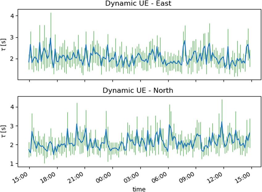
Hoffmann et al. EURASIP Journal on Wireless Communications and Networking     (2020) 2020:31                                        Page 5 of 19


  The satellite-receiver carrier phase distance measure-                 i
                                                                        φur = φui − φri = λ−1 rui − rri − Jui − Jri + Tui − Tri
ment can be now expressed as a measured fraction of the                           c
                                                                              + · (δtu −δtr +δtsi − δtsi ) + (Nui − Nri )+ ( ui − ri ).
wavelength cycle and an unknown integer number of full                           λ
cycles (integer ambiguity) [8]:                                                                                                   (7)
    φ(t) = ϕr (t) − ϕs (t − t) + N,                            (4)    When the UE is close enough to the reference station i.e.,
                                                                       less than 5 km of distance [16], the ionosphere and tro-
where N is an integer ambiguity, ϕr (t) is the local carrier
                                                                       posphere propagation errors are proven to be the same
replica phase, and ϕs (t − t) is the phase of the carrier
                                                                       (Jui − Jri = 0 and Tui − Tri = 0) [16], which can simplify (7)
received from satellite delayed by the propagation time
                                                                       to
t. When the receiver acquires a phase lock with the satel-
lite signal, then ϕr (t) = ϕs (t). Based on Eq. (3), Eq. (4) can                              c
                                                                             i
                                                                            φur   = λ−1 rur
                                                                                         i
                                                                                            + · δtur + Nur i
                                                                                                             + uri
                                                                                                                   ,              (8)
be expressed as                                                                               λ
                             r                                         where (•)iur = (•)iu − (•)ir .
     φ(t) = f t + N = + N,                                   (5)
                            λ
                                                                       5.1.2 Double difference
where r is the satellite-receiver distance in meters and λ
                                                                       While atmospheric errors and satellite clock bias are can-
is the carrier wavelength in meters. However, the mea-
                                                                       celed out by the single difference operation, UE and ref-
sured phase is distorted by the satellite and the receiver
                                                                       erence station clock biases (δtur ) may be canceled out
clock biases, δts , δtr , caused by the non-ideal synchroniza-
                                                                       by double difference. Having single difference related to
tion between satellites and receivers clocks. Secondly, the                                 i ), and single difference related to the
                                                                       the ith satellite (φur
measured phase suffers from the troposphere propagation                                  j
error (T, in meters) and the ionosphere propagation error              jth satellite (φur ), we can subtract them to get double
(J, in meters). Moreover, the receiver noise and the multi-            difference [8]:
path propagation introduces an additional error , so that                                                   c
                                                                                   − φur = λ−1 rur
                                                                         ij    i       j            i     j
the final measured carrier phase can be expressed as [8]               φur = φur                       − rur + · (δtur − δtur )
                                                                                                          λ
          r+J +T        c                                                     + Nur i       j
                                                                                      − Nur + ur    i
                                                                                                       − ur = λ−1 rur + Nur + ur ,
                                                                                                          j          ij      ij    ij
    φ=               + (δtr − δts ) + + N.                  (6)
               λ        λ
                                                                                                                                             (9)
Errors from the above equation can be split into the slow
and fast varying. Slow varying errors are atmospheric                              ij                  j
                                                                       where (•)ur = (•)iur − (•)ur .
delays (J, T) and clock biases (δts , δtr ), which can persist           It can be observed that the result of double difference
for tens of minutes [8]. Fast varying errors are related to            operation is affected only by an error caused by receiver
multipath propagation, and receiver noise ( ). They are                                                     ij
                                                                       noise and multipath propagation ur . Studies show that
claimed to be zero mean i.e. E[ ] = 0, and uncorrelated                the dominant distortion is introduced by the multipath
between measurements related to the different satellites               propagation. While receiver noise introduces about 1–
i.e. E[ i j ] = 0, for i  = j, and E[ i j ] = σφ2 , for i = j.        2 mm rms error, in the UE-satellite range the UE-satellite
Indices i, j denote satellite i, and j respectively [8].               rms range error caused by combined receiver noise and
                                                                       multipath propagation varies from 0.5 to 1 cm [8]. UE
5.1 Relative positioning                                               position estimation process utilizes a set of double dif-
To cancel out propagation errors (T, J) and clock biases                                                                 ij
                                                                       ference Eq. (9) to estimate integer ambiguities (Nur ) and
(δts , δtr ), the RTK is taking advantage of the so-called
                                                                       obtain final UE position.
relative positioning. The position of a user receiver is esti-
mated on the basis of its own measurements and the raw                 5.1.3 Double difference correlations
measurements from a reference base station of known                    As already mentioned fast varying errors of the car-
coordinates (possibly a 5G base station). The position is              rier phase measurement between UE and satellite ( ui
estimated as an offset to the reference station coordinates            in Eq. (7)) are uncorrelated and have the same variance
[8].                                                                   and zero mean. The undifferenced measurements error
                                                                       covariance matrix may be expressed as
5.1.1 Single difference

A general carrier phase measurement formula is given                   R = E [ φu − E[ φu ] ] [φu − E[ φu ] ]H = E u u H , (10)
by (6). Let us denote the phase of the ith satellite signal
measured at the UE as φui , and the phase of the ith satel-            where φu =[ φu1 , φu2 , . . . , φuK ]T , u =[ u1 , u2 , . . . , uK ]T and
lite signal measured at the reference station as φri . After           H denotes Hermitian transpose. After taking into account
subtracting Eq. (6), related with UE and reference station             our assumptions, it can be shown that, Eq. (10) can be
we get                                                                 simplified to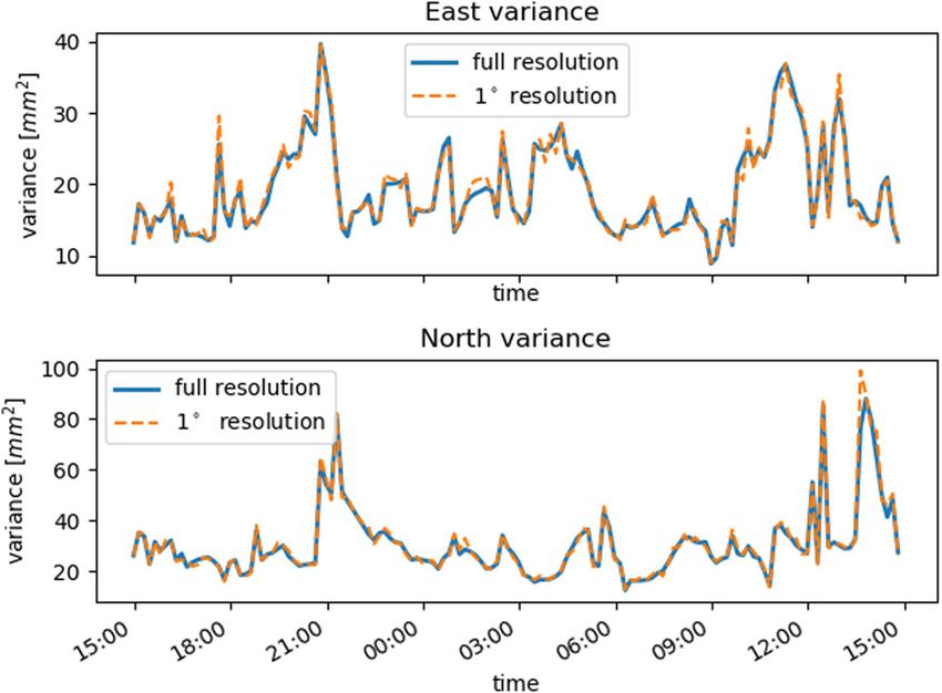
Hoffmann et al. EURASIP Journal on Wireless Communications and Networking        (2020) 2020:31                                     Page 6 of 19

    R = σu2 IK×K ,                                            (11)     5.1.4 Linear model for position estimation
                                                                       In the relative positioning, our target is to estimate the
where σu2 is the variance of the measured phase difference             position of UE relative to the reference station [8]:
related to the UE, I is the K × K identity matrix, and K
is the number of visible satellites. Note that the same rea-                  xur = xu − xr ,                                              (17)
soning can be applied in case of reference station-satellite
undifferenced phase measurement error covariance.
                                                                       where xr = (eastr , northr , upr )T is the vector of known
   The single difference operation from (7) can be pre-
                                                                       reference station coordinates, herewith given using east-
sented for the ith and the jth satellites using matrix
                                                                       north-up (ENU) coordinates system ( see Appendix A),
notation as
                                                                       xu = (eastu , northu , upu )T is the vector of UE coordi-
                                      ⎡ i ⎤
                                        φu                             nates (fixed over the measurement period but not known
                       1 −1 0 0 ⎢ φr ⎥⎢   i
             φur
               i                                                       at the UE), and xur is the UE relative position vector to
     φ sd =        =                  ⎣   j ⎥ .         (12)           be established by RTK. Let’s choose x0 (could be x0 = 0
               j
             φur       0 0 1 −1         φu ⎦
                                        φr
                                          j                            in practice [8]) as our initial estimate of the UE relative
                                                                       position vector xur , then [8]:
  Carrier phase measurements related to the UE and
reference station have different error variances σu2 , σr2 ,                  xur = x0 + δx,                                               (18)
respectively [16]. It can be shown that for any K visible
satellites single difference covariance matrix is given by             where δx is the unknown correction to the initial position
                                                    H                  estimate x0 .
    Rsd = E[ [ φ sd − E[ φsd ] ] [ φsd − E[ φsd ] ] ] =
                                                              (13)        Our target now is to introduce xur into the double
         = (σu2 + σr2 ) · IK×K .                                       difference given by (9). Figure 4 depicts the single differ-
                                                                       ence measurement UE (xu )-reference station (xr )-satellite
   In other words, single difference operation results are             geometry. When UE is ina smaller distance than 10 km
also uncorrelated, and their variances are two times                   from reference station we can assume that unit vector
greater.                                                               pointing from reference station to the satellite i (1ir ) is
   By taking three single differences related with the ith             equal to the unit vector pointing from UE to the satel-
             i ), the jth satellite (φ j ), and the kth satel-
satellite (φur                        ur                               lite i (1iu ) i.e., 1ir = 1iu [8]. Now rur
                                                                                                               i from Eq. (8) can be
        k
lite (φur ) we can write the corresponding pair of double              approximated as follows [8]:
differences in matrix notation [8]:
                                    ⎡ i ⎤                                    i
                                                                              rur = rui − rri = −1ir · xur .                               (19)
                 ji                       φ
               φur       1 −1 0 ⎣ ur
                                          φur ⎦ .
                                            j
     φ dd =           =                                  (14)
               φur
                 ki      1 0 −1
                                          φur
                                            k

 For a given pair of double differences the covariance
matrix can be expressed as

    Rdd = E[ [ φdd − E[ φdd ] ] [ φdd − E[ φdd ] ]H ] =
                          2 1                                 (15)
         = (σu2 + σr2 )       .
                          1 2

  It can be shown that for any K visible satellites the
double difference covariance matrix is given by [16]
                        ⎡                 ⎤
                          4 2 ··· 2
                        ⎢              .. ⎥
           (σu2 + σr2 ) ⎢
                        ⎢ 2 4           .⎥⎥
    Rdd =               ⎢  .              ⎥          (16)
                2       ⎣ ..      . .. 2 ⎦
                          2 · · · 2 4 K−1×K−1

As it can be seen, double differences are correlated even
if raw phase measurements and phases differences are
not. This observation, together with (16) will be used in
                                                                            Fig. 4 Geometry of the single difference measurements
Section 5.4.1 to obtain RTK covariance matrix.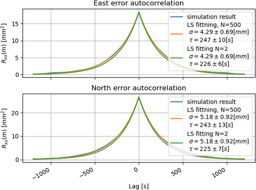
Hoffmann et al. EURASIP Journal on Wireless Communications and Networking         (2020) 2020:31                                      Page 7 of 19

 In the east-north-up (ENU) coordinates ( see Appendix                 the correction to the initial UE position estimate, to be
A) 1ir is given by [8]:                                                estimated.
                                                                       The target is to estimate the real-valued δx, and the inte-
   1ir = cos el(i) sin az(i) cos el(i) cos az(i) sin el(i) ,           gers n denoted as δ x̂ and n̂. This can be done by solving
                                                              (20)     the following least-squares optimization problem [8]:
where el(i) is the satellite i elevation angle and az(i) is the               min y − Gδ x̂ − n̂2                                             (27)
                                                                               n̂,δ x̂
satellite i azimuth angle.
                                ij                                     Methods for integer ambiguity resolutions are compre-
  On the basis of the (19) rur , from the double difference
given by (9), can be expressed as                                      hensively described in [8]. [27] discusses reducing time to
                                                                     integer ambiguity resolution with receiver random motion
     ij      i    j                 j
    rur = rur  − rur = − 1ir − 1r · xur .                  (21)        for smartphone grade GNSS antennas. For further com-
                                                                       puter simulations, n is assumed to be already estimated.
  Combining (18) and (21) we get [8]
                                                                     5.2 Undifferenced carrier phase measurement error
    ij             j
   rur = − 1ir − 1r · xur
                                                                       No zero error in UE localization estimate, i.e., δ x̂  = δx,
                                                                                             ij
                   j                 j                                 is caused by non-zero ur values in (24). The main source
       = − 1ir − 1r · x0 − 1ir − 1r · δx                      (22)
                                                                     of this error is multipath propagation. The double differ-
          ij           j                                                               ij
       = r0 − 1ir − 1r · δx,                                           ence errors ur are caused by raw phase measurements
                                                                       errors, e.g., ri and ui as visible in (7). These can be mod-
           ij
where r0 is estimated on the basis of x0 UE-reference                  eled by a Gauss-Markov (GM) process are shown in [27].
station distance.                                                      The GM process is specified by its variance σ 2 and its
  Combining (22) with (9) we obtain [8]                                correlation time - τ with the autocorrelation function for
                                                                     discrete time systems given by [28]
    φur = λ−1 r0 − λ−1 1ir − 1r · δx + Nur + ur . (23)
      ij         ij              j          ij    ij
                                                                                                   −|mTs |
                                                                            R (m) = σ 2 e          τ       ,                                  (28)
              ij    ij        ij                       j
  By setting yur = φur −λ−1 r0 , and gij = −λ−1 1ir − 1r ,
                                                                       where Ts stands for sample period, and m is an integer
(23) can be rewritten as a linear equation [8]:                        number representing autocorrelation sample index. It has
      ij                ij
     yur = gij · δx + Nur +
                               ij                                      to be noted that the sample period is here related with the
                               ur .                           (24)
                                                                       time intervals between consecutive position estimations
  Having K satellites visible, indexed 1, . . . , K, K − 1 inde-       and not the GNSS receiver sample rate.
pendent linear Eq. (24) can be formulated, e.g., by setting
j = 1 and i = 2, ..., K. Under the assumption that all mea-            5.2.1 Autoregressive model
surements are done in the same time period and that a                  A discrete stationary random process can be generated
single frequency receiver is utilized, these equations can             from white noise with the use of linear filter of transmit-
be presented in vector-matrix notation as follows [8]:                 tance H(z), as depicted in Fig. 5. If the stationary random
    ⎡ 21 ⎤            ⎡ 2        ⎤      ⎡ 21 ⎤ ⎡ 21 ⎤                  process is a GM process then H(z) consists only of the
      yur               1r − 11r           Nur             ur          poles. This case is called autoregressive (AR) model.
    ⎢ y31  ⎥          ⎢ 1 3 − 11 ⎥      ⎢  N   31 ⎥ ⎢ 31 ⎥
    ⎢ ur ⎥ −1 ⎢ r              r ⎥      ⎢ ur ⎥ ⎢ ur ⎥                    AR model parameters, i.e., the filter coefficients (ak ),
    ⎢ .. ⎥ =          ⎢     ..   ⎥ ·δx+ ⎢ .. ⎥ + ⎢ .. ⎥ ,              and the input white noise variance (σs2 ) can be computed
    ⎣ . ⎦       λ ⎣          .   ⎦      ⎣ . ⎦ ⎣ . ⎦
                                                                       with the following formula [29]:
        K1
      yur               1r − 1r
                         K     1           Nur K1         K1
                                                                                     ⎧
                                                          ur                                p
                                                              (25)                   ⎨ − k=1 ak Rxx (m − k), m > 0
                                                                                              p
                                                                          Rxx (m) = − k=1 ak Rxx (−k) + σs2 m = 0 , (29)
or                                                                                   ⎩
                                                                                                 R∗xx (−m)          m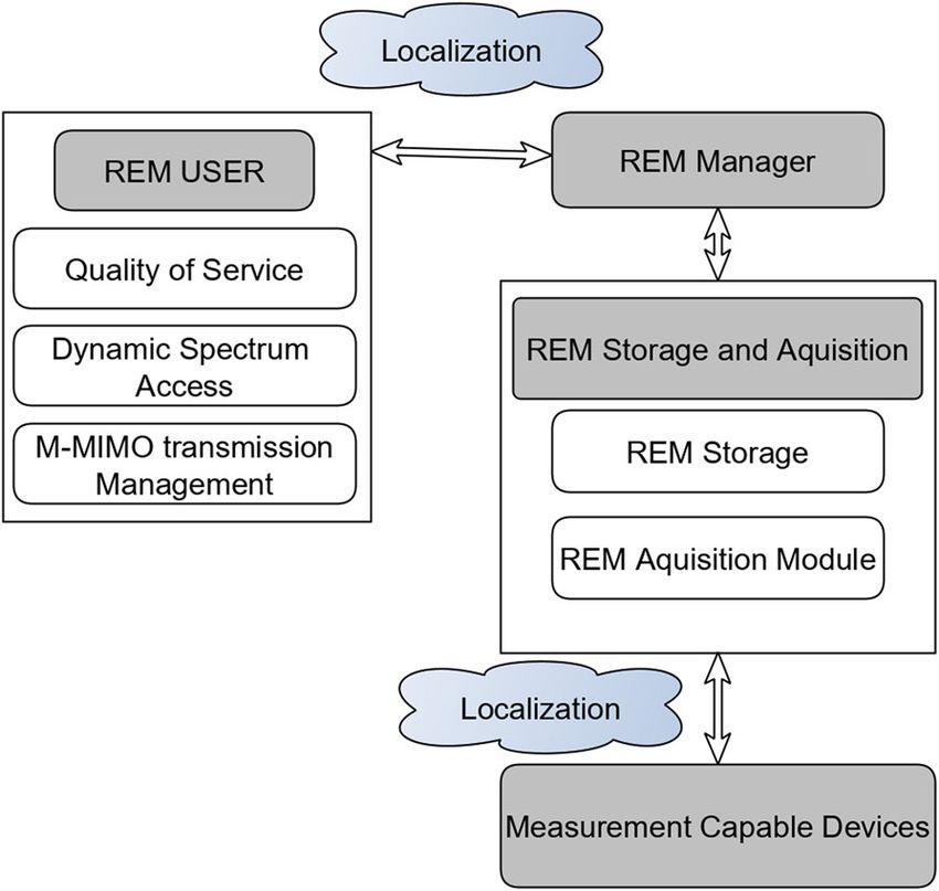
Hoffmann et al. EURASIP Journal on Wireless Communications and Networking (2020) 2020:31 Page 8 of 19
⎡ ⎤⎡ ⎤ ⎡ ⎤
5.2.2 Autoregressive model parameters for Gauss-Markov R̂xx (0) R̂xx (1) · · · R̂xx (p) 1 σs2
process ⎢ R̂xx (1) R̂xx (0) ⎥ ⎢ ⎥
· · · R̂xx (p − 1) ⎥ ⎢ a1 ⎥ ⎢ 0 ⎥
⎢
⎢ . ⎥⎢ . ⎥ = ⎢ ⎥.
⎦ ⎣ .. ⎦ ⎣ 0 ⎦
Adopting a first order model AR(1) for the GM process .. ..
⎣ .. . ··· .
and writing (29) for p = 1, and combining with (28) results 0
to the following set of equations: R̂xx (p) R̂xx (p − 1) · · · R̂ (0)
xx a
p
⎧ −|mTs | −|(m−1)Ts |
(35)
⎪
⎨ σ 2 e τ = −a1 σ 2 e τ m>0
−Ts Consider now extending autocorrelation matrix to dimen-
⎪ σ = −a1 σ e
2 2 τ + σs 2 m=0 , (30)
sions N × p, where N is number of the autocorrelation
⎩ ∗
Rxx (m) = Rxx (−m) m 0, we can write |mTs | = will be estimated using standard x(n) variance estimator,
mTs , and |(m − 1)Ts | = mTs − Ts . Equation (30) can be and some minor transforms (35) can be rewritten as
simplified to ⎡ ⎤⎡ ⎤
R̂xx (0) R̂xx (1) · · · R̂xx (p − 1) a1
⎧ −mTs ⎢ R̂xx (1) ⎥ ⎢ a2 ⎥
⎪
−mTs Ts
= −a1 e τ e τ m > 0 ⎢ R̂xx (0) · · · R̂xx (p − 2) ⎥⎢ ⎥
⎨e τ
⎢ .. .. .. ⎥ ⎢ . ⎥=
−Ts
σ 2 1 + a1 e τ = σs2 m = 0 . (31) ⎣ . . ··· . ⎦ ⎣ .. ⎦
⎪
⎩ ∗
R (m) = R (−m) m < 0 R̂xx (N −1) R̂xx (N −2) · · · R̂xx (N −p) ap
⎡ ⎤
After further transforms, we can obtain R̂xx (1)
⎢ R̂xx (2) ⎥
Ts ⎢ ⎥
a1 = −e− τ = −⎢ .. ⎥
(32) ⎣ . ⎦
−2Ts
σs2 = σ 2 1 − e τ R̂xx (N)
which can be used directly for the generation of the (36)
required GM process. For the considered first order AR model, (36) simplifies to
⎡ ⎤ ⎡ ⎤
5.2.3 Fitting Gauss-Markov process parameters R̂xx (0) R̂xx (1)
Now a reverse problem can be considered: having sam- ⎢ R̂xx (1) ⎥ ⎢ R̂xx (2) ⎥
⎢ ⎥ ⎢ ⎥
ples of the random process x(n), the target is to model it ⎢ .. ⎥ · a1 = − ⎢ .. ⎥, (37)
⎣ . ⎦ ⎣ . ⎦
with the GM process and obtain parameters: σ̂ 2 and τ̂ .
R̂xx (N − 1) R̂xx (N)
While variance σ̂ 2 can be computed directly from x(n)
samples, the estimation of the correlation time is more by introducing
complicated. ⎡ ⎤
R̂xx (0)
By transformation of (32), τ̂ is given by ⎢ R̂xx (1) ⎥
⎢ ⎥
−Ts d=⎢ .. ⎥, (38)
τ̂ = . (33) ⎣ . ⎦
ln(−a1 )
R̂xx (N − 1)
The filter coefficient a1 can be estimated based on (29)
⎡ ⎤
as [29]: R̂xx (1)
⎢ R̂xx (2) ⎥
R̂xx (1) ⎢ ⎥
a1 = − , (34) c=⎢ .. ⎥ (39)
⎣ ⎦
R̂xx (0) .
R̂xx (N)
where R̂xx (m) is the estimated autocorrelation function of
x(n). This approach is sufficient when x(n) is an ideal GM equation (37) can be written in vector notation as
process as it is impossible to create over-determined set d · a1 = −c. (40)
of equations from (29) in that case. In practice simulation
The estimation of a1 , using least squares criterion is
results presented in further sections (e.g., Fig. 12) would
given by
have autocorrelation not being ideal function described
−1
by (28). â1 = dT d dT (−c). (41)
5.2.4 Proposed a1 estimation algorithm As d is a vector, (41) can be rewritten as
In such a non-ideal case it is reasonable to use more than
two autocorrelation function samples. Equations (29) can dT
â1 = − c, (42)
be rewritten in matrix notation as [29]: d22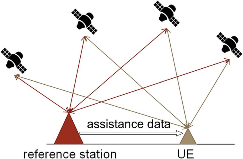
Hoffmann et al. EURASIP Journal on Wireless Communications and Networking      (2020) 2020:31                               Page 9 of 19

where  • 2 denotes the Euclidean norm. Now τ̂ can be                            – Inclination (i ), angle measured between the
estimated from (33).                                                                satellite orbital plane and the Earth’s
                                                                                    equatorial plane.
5.3 GPS satellites orbits prediction                                              – Longitude of the ascending node ( ), angle in
Apart from UE (reference station)-satellite range errors,                           Earth’s equatorial plane measured between the
also the geometry of the visible satellites influences the                          vernal equinox direction, and the ascending
final position error in RTK. This is visible, e.g., in (27) by                      node which is the point on the satellite’s orbit
G varying with the satellites geometry. Because GPS is the                          where it crosses the equatorial plane, moving
most popular GNSS systems, in this paper, we will focus                             in the northerly direction.
on estimating GPS satellites constellation. However, sim-
                                                                            • The following single parameter characterizes
ilar algorithms could be used for other systems, e.g., for
Glonass [30].                                                                 orientation of the ellipse in orbital plane:

                                                                                  – Argument of perigee (ω), angle in the plane of
5.3.1 Ideal elliptical orbit parameters
                                                                                    the orbit, measured between the ascending
For simplicity, it is assumed that the GPS satellite motion
                                                                                    node and the perigee, which is point in the
can be modeled with ideal elliptical orbit. This approach
                                                                                    satellite orbit, where the satellite is closest to
results in 1–2 km standard deviation of the error in esti-
                                                                                    the center of the Earth.
mating satellites position [8], but remains good enough
for evaluation of satellites constellation geometry influ-                  • The last Keplerian orbit parameter determines
ence on UE position error. The influence of satellites                        satellite position on its orbit in given time epoch:
position accuracy on the performance of proposed UE
localization error is evaluated by simulations in Section 6.                      – True anomaly (ν), angle measured in orbital
Satellite position at specified time epoch on such orbit can                        plane between perigee, and the satellite
be described with Keplerian elements defined below (see                             position at given time.
Fig. 6) [8]:
                                                                         5.3.2 System effectiveness model almanac
  • GPS satellite ellipse orbit size and shape can be                    Each GPS satellite distributes simple ephemerides (Kep-
    described by two parameters:                                         lerian orbit parameters) for whole constellation (so-called
                                                                         almanac). Receiving full almanac data takes 12.5 min [8].
          – Semi-major axis (a )                                         A more practical and flexible approach is to use Sys-
          – Eccentricity (e )                                            tem Effectiveness Model (SEM) almanac available online
  • The next two parameters are describing relation                      instead of obtaining almanac transmitted by a GPS satel-
    between orbital plane, and the Earth’s equatorial                    lite. The definition of the SEM almanac content can be
    plane, and the direction of vernal equinox:                          found in [31].

                                                                         5.3.3 Satellite position computation algorithm
                                                                         With the data from SEM almanac, it is possible to obtain
                                                                         a coarse position of all satellites in the GPS system con-
                                                                         stellation. The satellite position computation algorithm is
                                                                         presented below [32].

                                                                            1. In the first step, two World Geodetic System 84
                                                                               (WGS 84) constants must be introduced [32]:

                                                                                                          m3
                                                                                   μ = 3.98605 × 10¹⁴        ,                       (43)
                                                                                                          s2

                                                                               which is WGS 84 value of the Earth’s gravitational
                                                                               constant for GPS users [32]. The second constant is
                                                                               the WGS 84 value of the Earth’s rotation rate given
                                                                               by
 Fig. 6 Characterization of an ideal orbit and satellite position by
 Keplerian elements, where the reference direction is the vernal                                                  rad
                                                                                   ˙ e = 7.2921151467 × 10⁻⁵                         (44)
 equinox direction, and the plane of reference is the Equatorial plane                                             s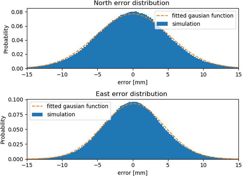
Hoffmann et al. EURASIP Journal on Wireless Communications and Networking       (2020) 2020:31                                    Page 10 of 19

 2. The satellite mean motion (n0 ) is computed using                          (ĩ0 = π · i0 , and δ̃i = π · δi). Next, the longitude of
    square root of semi major axis from SEM almanac                            the ascending node is
     √
    ( a):

                 μ                                                                   p   = ˜ 0 + ( ˜˙ − ˙ e )t − ˙ e tas ,               (53)
       n0 =                                          (45)
                a3
 3. Now, the difference between almanac time (defined                          where ˜ 0 = π · 0 and ˜˙ = π · ˙ , because 0 and ˙
    by GPS Week Number - taw and GPS time of                                   are given in SEM almanac in the units of semicircles,
    applicability - tas ), and the desired time (defined by                    and semicircles/second, which are converted to the
    weeks number - tdw and seconds number - tds ) is                           units of radians and radians/second, respectively.
    computed from the following formula:                                    9. The final step is to obtain the GPS satellite position
                                                                               in ECEF coordinates with the following formulas:
          t = tds − tas + (tdw − taw ) · s,                  (46)
    where s is the number of seconds in a single week.                             ⎧
                                                                                   ⎨ xECEF = x cos p − y cos i sin            p
 4. In this step, mean anomaly for desired time is                                   y     = x sin p + y cos i cos                        (54)
                                                                                                                              p
    obtained using mean anomaly for almanac time (M0 )                             ⎩ ECEF
                                                                                             zECEF = y sin i
    from SEM almanac, and the values obtained from
    Eq. (45) and (46):                                                 5.3.4 Algorithm implementation and validation
                                                                       The presented GPS satellite position estimation algorithm
          M = M̃0 + n0 · t,                                  (47)
                                                                       had been implemented in Python programming language.
    where M̃0 = π · M0 , is converted to radians (1                    To validate the implemented algorithm, visible satellite
    semicircle = π radians), as SEM gives M0 in the                    list had been captured from USB-GPS antenna. USB
    units of semicircles.                                              antenna outputs the data via serial port using National
 5. Eccentric anomaly (E measured in radians) can be                   Marine Electronics Association (NMEA) protocol. To
    found by solving the so-called Kepler’s equation                   this end, a C++ program has been developed to cap-
    given by                                                           ture only data frames containing information about visible
                                                                       satellites and log them to text file (see Fig. 7). Satellite
                                                                       coordinates are the azimuth (az) and the elevation (el)
          M = E − e sin E,                                    (48)
                                                                       angles seen from GPS antenna position (52.3921476900N,
    where e is the eccentricity from SEM almanac.                      16.7982299300E). Observations were performed in a 24 h
    Kepler’s equation can be iteratively solved with one               period between 29 and 30 of December 2018.
    of the several available methods [33].                                Results of the comparison between the computed and
 6. Having eccentric anomaly calculated, the GPS                       the captured satellites coordinates are presented in Fig. 8.
    satellite position on the Keplerian orbit can be                   The former are derived by using the algorithm described
    defined by true anomaly:                                           in Section 5.3.3, with SEM almanac obtained 28 Decem-
                     √                                                 ber 2018 19:56:48 UTC, while the latter are extracted
                       1 − e2 sin E                                    from NMEA messages. There are two sources of errors:
        ν = arctan                  ,                 (49)
                        cos E − e                                      the first source of error is related to the 1◦ quantiza-
     and the radius by                                                 tion of NMEA data (even though internally GPS receivers
                                                                       use much more accurate satellites positioning), while
          r = a(1 − e cos E)                                  (50)
                                                                       satellite coordinates computed with SEM almanac data
 7. After transformation of the satellites coordinates                 domain is continuous. Up to 0.5◦ of error can be expected.
    from radial to Cartesian, we get                                   The second source of errors is related to the computing
                                                                      satellites coordinates, i.e., the utilized satellites position
          x = r cos (ν + ω)
                                                       (51)            forecasting, on the basis of ideal elliptic orbit, while in
          y = r sin (ν + ω)
                                                                       fact there are some temporary deviations in the satellites
 8. Next, the satellite coordinates in Keplerian orbit                 orbits.
    plane are transformed to ECEF ( see Appendix A)                       As it can be observed in Fig. 8, satellites orbits predic-
    coordinates. Two parameters are obtained to perform                tion error doesn’t grow over the analysed time period.
    this operation. First, the inclination is given by                 This turns satellite constellation obtained on the basis of
                                                                       the algorithm described in Section 5.3.3 to be a reasonable
          i = ĩ0 + δ ĩ,                                     (52)
                                                                       tool for 24 hours long simulations. Also prediction errors
     where both i0 and δi are given in the SEM almanac in              around 1◦ seems to have no significant impact on the error
     semicircles units and must be converted to radians                modeling, as it is shown in Section 6.2.3.
Hoffmann et al. EURASIP Journal on Wireless Communications and Networking (2020) 2020:31 Page 11 of 19
Fig. 7 Example set of the visible satellites coordinates (1◦ resolution)
extracted from NMEA data captured by G-Mouse USB antenna and
logged into text file
5.4 RTK error estimation simulation environment
A block scheme illustrating initial framework for UE local-
ization error modeling in RTK system under open-sky
conditions is presented in Fig. 9. The simulation envi-
ronment consists of several functional blocks presented Fig. 9 Block scheme illustrating simulation environment for the RTK
in previous subsections: Gauss-Markov noise generators positioning error estimation
(Section 5.2.2), SEM almanac-based satellites orbit pre-
diction (Section 5.3.3), and linear model for position
estimation (Eq. (26)). for position estimation to formulate Eq. (27) under the
For a given time instance, a list of visible satellites is assumption of having resolved integer ambiguities. Finally
computed on the basis of SEM almanac with the 7◦ ele- the position error is computed as the difference between
vation cutoff angle, i.e., satellites close to the horizon true UE coordinates, and the ones computed from the
are treated as not visible for the UE receiver [8]. Next, noised reference station-satellite and the UE-satellite
on the basis of reference station position, and UE "true" ranges.
position satellite-reference station, and the satellite-UE
ranges are computed for each visible satellite. With the 5.4.1 RTK positioning error covariance matrix estimation
use of the independent GM process generators (with the In the other less computationally complex approach, the
given fix parameters: variance σ 2 and correlation time RTK positioning error covariance matrix may be esti-
τ ) obtained ranges are noised. Noised ranges and visi- mated with the analytic formula, describing the least
ble satellites coordinates are then used in linear model squares estimator covariance matrix and given by [8]
−1 −1
cov(δx) = GT G GT · Rdd · G GT G , (55)
where G is the satellite-reference station-UE geometry
matrix (Eq. (26)) , and the Rdd is the double difference cor-
relation matrix (Eq. (16)). Unfortunately, in this approach,
random variables variances, can be only obtained, with no
information on the positioning error distribution. More-
over, autocorrelation function cannot be estimated.
6 Simulation results and discussion
For evaluation purposes, the environment described in
Section 5.4 is implemented in python programming lan-
guage. Several computer simulation experiments have
been performed for various sets of input parameters.
Three places globally had been chosen for simulations.
These are listed in Table 1. Loc1 refers to the first
Fig. 8 Comparison between visible satellites coordinates computed author’s home near Poznan in Poland, Loc2 to the point
with algorithm from Section 5.3.3, and those obtained from NMEA where prime meridian intersects equator, and Loc3 to
data provided by USB antenna
the Huawei headquarters in the Chinese city of Shenzen.Hoffmann et al. EURASIP Journal on Wireless Communications and Networking (2020) 2020:31 Page 12 of 19
Table 1 Coordinates of the reference station and UE used in the simulation runs; UE position is computed in 1 s inter-
simulations vals. During the whole simulation experiment, the satellite
Scenario name Reference station UE geodetic coordinates constellation is continuously changing.
geodetic coordinates
Loc1 52.3921476900N 52.3911476900N 6.1.1 Localization error distribution
16.7982299300E 16.7972299300E The first field of study for this simulation scenario is
117.19200 m 117.19200 m
localization error empirical probability density function.
Loc2 0.00000000000N 0.00100000000N Figure 10 present the localization error distribution in the
0.00000000000E 0.00100000000E
0.00000 m 0.00000 m east and north directions with fitted Gaussian functions.
Loc3 22.6530360000N 22.6540360000N
As can be seen, distributions have shape of the Gaussian
114.060506000E 114.061506000E distribution.
110.00000 m 110.00000 m
6.1.2 Autocorrelation analysis
Apart from the localization error distribution, also the
The UE-reference station distance is chosen to be 130 m, autocorrelation functions are analyzed. If the localization
157 m, and 151 m for Loc1, Loc2, and Loc3, respectively. error can be described by GM process, autocorrelation
Choosing such distances ensures the UE and reference function can be given by Eq. (28). Here, it appears the
station are affected by the same atmospheric propaga- problem of fitting GM process parameters already dis-
tion delays, as explained in Section 5.1. This is reasonable cussed in Section 5.2.3. Correlation time is estimated
for a dense 5G network and allows for the simplification with the use of (42). However, the number of the utilized
of error modeling by assuming that errors related with autocorrelation function samples must be established.
ionosphere and troposphere delays are equal at UE and Figure 11 illustrates RMSE between the empirical autocor-
reference station. relation function and fitted GM autocorrelation function
The input parameters for GM process generators, which while changing the number of the empirical autocorrela-
models the UE-satellite, and reference station-satellite dis- tion function samples (N) used in the fitting process. As
tance error are specified based on the measurements it can be seen, higher N results in lower RMSE. How-
with the use of smartphone-grade and survey-grade GNSS ever, the improvement is negligible for N > 500. As
antenna, respectively, under open-sky conditions done in such N = 500 is used in all subsequent simulation
[16]. The values of the GM process parameters are shown experiments.
in Table 2. Static correlation time refers to the scenario Autocorrelation functions for east and north directions
when the receiver antenna does not move, i.e., the ref- are presented in Fig. 12. In each figure there is the autocor-
erence station is always static. Dynamic correlation time relation obtained from the simulation results, and two fit-
refers to the scenario, when UE moves randomly within ted GM processes: using Eq. (42) with N = 500 and using
the GPS L1 carrier signal wavelength. The trajectory of the (34). It can be seen that the fitted GM process autocorre-
receiver is modeled as a GM process and has an average lation function approximates the one obtained from sim-
speed of 7.65 kmh [16].
ulation results very well. This, along with the localization
In all simulations, SEM almanac is utilized (almanac error samples following the Gaussian distribution, leads
date: 28 December 2018 19:56:48 UTC). For all simula-
tions, start date is 29 December 2018 14:58:09 UTC, and
end date is 30 December 2018 14:58:09 UTC. Longer than
a 24 h simulation period is not necessary due to the fact
that visible satellites constellation repeats every 23 h and
56 min [8].
6.1 Continuous 24 h scenario
The first computer simulation is performed for Loc1,
with static GM noise parameters. There are 15, 24-h-long
Table 2 GM process parameters for modeling of undifferenced
carrier phase measurement error for a static reference station
σ τ - static τ - dynamic
Reference station 2.5 mm 100 s —
UE 6 mm 300 s 0.01 s Fig. 10 Localization error distributionHoffmann et al. EURASIP Journal on Wireless Communications and Networking (2020) 2020:31 Page 13 of 19
influence of the visible GPS satellites geometry on the
RTK localization error at a given time and geographical
position.
Simulation is performed in a "step mode." Every single
step is related to a constant satellites constellation, and
15 independent simulation runs, each utilizing a differ-
ent random generator seeds. During each simulation run,
3600 UE position error samples are collected at 1 Hz sam-
pling frequency. From 29 December 2018 14:58:09 UTC to
30 December 2018 14:58:09 UTC, a new satellite constel-
lation is computed every 10 min, and the corresponding
simulations are performed, resulting in 144 steps. The
simulations are performed for all locations in Table 1,
static reference station and static/dynamic UE.
Fig. 11 Dependence between number of utilized autocorrelation 6.2.1 Variance analysis
function samples used for GM process fitting and the resultant RMSE Firstly, RTK localization error variance obtained with
the use of the simulation environment presented in
Section 5.4 is compared with the one estimated using
to the conclusion that the UE localization error in RTK analytical formula (55), as it is depicted in Fig. 13 for Loc1.
system may be modeled as a GM process. The variance obtained with (55) visibly overlap with simu-
To check if there is a correlation between RTK localiza- lation results for the dynamic UE. In the static UE scenario
tion error in the east and north directions, the correlation variance obtained on the basis of simulation and Eq. (55)
coefficient (see [34]) has been computed with the result differs more. This can be caused by longer correlation
of − 0.0669. A correlation coefficient close to 0 leads time (300 s) that results in smaller number of independent
to the conclusion that east and north localization errors localization error samples over the simulated period.
are uncorrelated and can be modeled independently. However, it can be stated that the estimated variance is
With other words independent GM process generators independent of UE motion. Additionally, it is confirmed
can be utilized to produce east and north localization that the localization variance can be generated using (55)
error. instead of performing full system simulations. In Fig. 14,
localization error variances obtained on the basis of (55)
6.2 Step 24 h scenario for all considered geographical localizations are compared
All previous simulations revealed that RTK localization for the same time instances. It can be observed that the results
errors in east and north directions are uncorrelated and differ significantly. This implies that RTK localization
may be modeled as a GM process. Next, we study the error variance depends on the visible satellites geometry.
Fig. 12 Autocorrelation of the localization error in Loc1, computed on
the basis of: simulation, Eq. (42) with N = 500, and Eq. (34). σ and τ Fig. 13 Comparison between RTK localization error variance in Loc1
parameters are estimated with 95% confidence intervals obtained from simulations, and computed with Eq. (55)Hoffmann et al. EURASIP Journal on Wireless Communications and Networking (2020) 2020:31 Page 14 of 19
Fig. 14 Comparison between RTK localization error variances Fig. 16 Correlation time obtained on the basis of simulation results in
obtained at different geographical localization Loc1,and for the static UE
reject or not hypothesis, the ANOVA test output, i.e., p
6.2.2 Correlation time analysis value, is compared with the so-called significance level (α),
Apart from the variance, the GM process is also described i.e., the probability of rejecting hypothesis which is actu-
by correlation time. As an example, simulation results ally true (typical α value is 0.05) [35]. The hypothesis may
obtained for Loc1 are presented in Fig. 15, in the case be rejected with significance level α when pvalue < α. The
of dynamic UE, and Fig. 16, in the case of static UE. In corresponding ANOVA results are presented in Table 3.
both presented examples, the correlation time seems to The hypothesis is rejected only in the case with dynmic
be randomly fluctuating around a mean value, with no UE in east direction and Loc2.
dependence of daytime or geographical localization. This In conclusion, the RTK localization error correlation
hypothesis is validated by means of analysis of variance time depends only on undifferenced carrier phase mea-
(ANOVA) statistical test on the correlation time data. surement error and is independent of daytime and geo-
ANOVA is a statistical test that allows to check if sev- graphical localization, i.e., visible satellites constellation.
eral data sets have statistically equal means, by analysis of The mean values of correlation time, averaged over all
their variance [35]. The ANOVA test has been indepen- 144 steps, for all of studied geographical locations are
dently performed for each simulation scenario and for all presented in Table 4. For dynamic UE localization error
data sets related with static and dynamic UE respectively.
The aim of the ANOVA test was to reject or not hypothe- Table 3 ANOVA statistical tests results for localization error
sis h0 that all data sets (correlation time over daytime and correlation times
geographical localization) have the same mean value. To Dataset p value h0
Dynamic UE
Loc1 - east 0.57 Not rejected
Loc1 - north 0.10 Not rejected
Loc2 - east 0.014 Rejected
Loc2 - north 0.93 Not rejected
Loc3 - east 0.19 Not rejected
Loc3 - north 0.17 Not rejected
all (excluding Loc2 - east) 0.17 Not rejected
Static UE
Loc1 - east 0.30 Not rejected
Loc1 - north 0.42 Not rejected
Loc2 - east 0.43 Not rejected
Loc2 - north 0.36 Not rejected
Loc3 - east 0.12 Not rejected
Fig. 15 Correlation time obtained on the basis of simulation results in Loc3 - north 0.71 Not rejected
Loc1 and for the dynamic UE all 0.25 Not rejectedHoffmann et al. EURASIP Journal on Wireless Communications and Networking (2020) 2020:31 Page 15 of 19
Table 4 RTK east and north localization error correlation times, localization error in urban environment, i.e., without tak-
averaged over 24 h with 95% confidence intervals
ing into account NLoS UE-satellite signals propagation
Localization East error correlation North error correlation or cycle-slip occurrence. This can be done by increasing
time [s] time [s]
the elevation cutoff angle αel from the default 7◦ to the
Dynamic UE value related to street geometry: width W and neigh-
Loc1 2.0429 ± 0.0404 2.1172 ± 0.0441 boring buildings height H as depicted in Fig. 18. This
Loc2 2.0392 ± 0.0388 1.9983 ± 0.0403 approach mimics signals from some GNSS satellites being
Loc3 2.0517 ± 0.0414 2.0738 ± 0.0421 blocked by buildings.
Dependence between street geometry of width W, and
Static UE
height H, and elevation angle cutoff αel is given by
Loc1 257.04 ± 4.78 255.94 ± 5.04
Loc2 251.96 ± 4.50 258.45 ± 4.90
2H
Loc3 251.84 ± 4.62 255.97 ± 4.70 αel = arctan . (56)
W
correlation time in both east and north directions can be A simulation was performed to estimate RTK local-
assumed to be 2 s. The mean value of the correlation times ization error variance in Loc1 while changing αel . The
in the case of static UE (in both east and north direc- elevation angle was increased to the value of 18◦ that cor-
tions) is 255.2 s and fits in the confidence intervals in responds to the W H
street geometry ratio equal to 0.162.
Table 4. Results are depicted in Fig. 19. As expected, a higher ele-
vation cutoff angle causes fewer satellites visibility. This
6.2.3 Visible satellites coordinates resolution analysis
finally results in a larger localization error in relation to
The proposed RTK localization error framework rely on
the one obtained with default 7◦ elevation cutoff angle.
visible satellites coordinates. The utilized satellites local-
ization prediction uses SEM almanac introducing typi-
7 Final RTK localization error modeling algorithm
cally 1–2 km error (as mentioned in Section 5.3). The aim
On the basis of the previous results a RTK localization
of this section is to verify whether degradation of satellites
error model for smartphone-grade GNSS antenna under
coordinates accuracy significantly impacts the final UE
open-sky conditions is proposed. Simulation experiments
localization error. On the basis of Eq. (55), the localization
from Section 6.1 shown that RTK localization errors in
error variance for Loc1 geographical localization is com-
both east and north directions are uncorrelated and may
puted with the visible satellites coordinates rounded to 1◦
be modeled as a GM process. Further simulations from
and compared with the full-accuracy results in Fig. 17. As
Section 6.2 proved that there is a dependence between
it can be seen, the presented results are almost identical.
localization error variance and geographical localization
6.2.4 Adaptation of the proposed scheme for urban and daytime as a result of the different visible satellites
environment geometry. The localization error correlation time seems
In addition, the proposed RTK localization error frame- to be related to the UE motion. The proposed model
work may be applied to provide initial estimate of the considers correlation time for two scenarios. First, it is
appropriate for static UEs, e.g., people sitting on the bench
in a park. Second, it can be applied for dynamic UEs,
e.g., fast walking pedestrians. However, additional studies
would be required to obtain a mathematical formula to
Fig. 17 RTK localization error variance, computed with Eq. (55), for Fig. 18 RTK LoS under urban conditions, modeled by adjusting
non-rounded and rounded to 1◦ satellites coordinates (az, el) in Loc1 elevation cutoff angle αal to the street geometry: width W and height HYou can also read