Exploring Factors that Influence Individuals' Choice Between Internal Combustion Engine Cars and Electric Vehicles

Page created by Willard Yang

Cars & Machinery

English

Like
Share
Embed
Fullscreen
Slides
Download HTML
Download PDF
Abuse

←

→

Page content transcription

If your browser does not render page correctly, please read the page content below

1 of 23

Exploring Factors that Influence Individuals’
Choice Between Internal Combustion Engine Cars
and Electric Vehicles
Dominik Bucher1, Henry Martin 1, Jannik Hamper1, Atefeh Jaleh2,
Henrik Becker2, Pengxiang Zhao1 and Martin Raubal1
1
Institute of Cartography and Geoinformation, ETH Zurich
2
Institute for Transport Planning and Systems, ETH Zurich
{dobucher, martinhe, hamperj, pezhao, mraubal}@ethz.ch
henrik.becker@ivt.baug.ethz.ch, atefe.jaleh@gmail.com

Abstract. The adoption of electric vehicles has the potential to help decarboniz-
ing the transport sector if they are powered by renewable energy sources. Limi-
tations commonly associated with e-cars are their comparatively short ranges and
long recharging cycles, leading to anxiety when having to travel long distances.
Other factors such as temperature, destination or weekday may influence people
in choosing an e-car for a certain trip. Using a unique dataset of 129 people who
own both an electric vehicle (EV) as well as one powered by an internal combus-
tion engine (ICE), we analyze tracking data over a year in order to have an em-
pirically verified choice model. Based on a wide range of predictors, this model
tells us for an individual journey if the person would rather choose the EV or the
ICE car. Our findings show that there are only weak relations between the pre-
dictor and target variables, indicating that for many people the switch to an e-car
would not affect their lifestyle and the related range anxiety diminishes when
actually owning an electric vehicle. In addition, we find that choice behavior does
not generalize well over different users.

Keywords: Electric Vehicle, Transport Mode Choice, Mobility.

1 Introduction

Individual fossil fuel based transportation is a major contributor to greenhouse gas
(GHG) emissions and thereby a serious threat to the global ecosystem [8, 36, 16]. With
the imminent threat of climate change, the decarbonization of individual transportation
has become one of the important questions of our time. In that context, renewable en-
ergy generation combined with electric vehicles (EVs) has great potential as it leads to
significantly lower GHG emissions than internal combustion engine (ICE) cars [33, 14,
12]. In line with this, many major car manufacturers started adding EVs to their product
range and the share of EVs in global car sales is projected to be at around 35% by 2040
[19]. However, while electrification is currently the most promising path towards a
more sustainable transportation sector, the large-scale adaption of EVs is a slow process
and people still associate EVs with uncertainties: “How far can I drive with a fully
charged vehicle? Will I have charging stations on the way to my destination? How

AGILE: GIScience Series, 1, 2020.
Full paper Proceedings of the 23rd AGILE Conference on Geographic Information Science, 2020.
Editors: Panagiotis Partsinevelos, Phaedon Kyriakidis, and Marinos Kavouras
This contribution underwent peer review based on a full paper submission.
https://doi.org/10.5194/agile-giss-1-2-2020 | © Authors 2020. CC BY 4.0 License.

2 of 23

quickly does the battery wear out?” Such questions are commonly at the center of dis-
cussion when someone considers switching to an EV. As a result of this mistrust, EVs
are often bought as an additional second car, complementary to the ICE car [13]. The
resulting group of people is over-equipped with mobility tools and potentially has to
decide for every trip whether to use the EV or the ICE car. A closer look at their mo-
bility behavior can offer valuable insights about the choice between these two transport
modes. Knowing when and why people prefer the ICE car over the EV may reveal some
of the factors that are still slowing down EV adaption. Furthermore, being able to pre-
dict this choice can be used to optimize smart charging applications or also to offer
automated and personalized route planning.

In this study, we analyze a tracking dataset of 129 persons who own an ICE car and
an additional (compact class) EV as second car. We control their mobility choice be-
havior on three types of factors: trip descriptors (e.g., length, duration or trip purpose),
socio-demographic factors and spatio-temporal context data. Given the limited range
of EVs and the well-known issue of range anxiety [7], we hypothesize that we can
explain the mobility choice by the distance of the trip as the primary influencing factor,
followed by (less important) influencing variables such as the duration of the planned
trip (e.g. several hours vs. several days), the temperature (due to an increased heating
demand the range of EVs is decreased in cold weather), or the weekday of the departure
(e.g., on weekends, people might want to use the ICE car due to being more spacious
or luxurious than the compact class EV).

We find that while these factors can indeed be used to infer the transport mode
choice, their impact on the overall prediction accuracy is small, and the herein evaluated
models are of comparably low explanatory power. It turns out that for most of their
travels, the participants of the study chose the EVs independently of the predictors an-
alyzed within this paper, and instead make their choice largely dependent on other con-
textual factors (such as traveling with the family). This is good news for everyone con-
sidering buying an electric vehicle: In practice, for most trips performed, people do not
seem to prefer one of the drive technology over the other. As part of our experiments,
we additionally evaluated how well our models generalize across different users. We
found that the fitted models are hardly transferable to unseen users but that the
knowledge about individual users greatly increases the prediction accuracy for these
users. This is an additional hint that while there are only weak relations between the
examined features and the mode choice, the users’ mode choice behavior is unique and
regular.

The rest of this paper is structured as follows: In Section 2, existing mode choice
models are evaluated, in particular with respect to EVs. Section 3 introduces the dataset
in more detail and explains the various preprocessing steps. The different models eval-
uated are presented in Section 4, and their results and predictive power in Section 5.
Finally, we discuss and conclude the paper in Section 6.

3 of 23

2 Related Work

2.1 Transport Mode Choice
Choices of transport modes differ widely, between individuals as well as between coun-
tries. For example, the work by Zhao et al. [37] developed a clustering-based frame-
work to understand individuals’ travel mode choice behavior in multi-modal transpor-
tation. It is shown that the users exhibit different patterns in spending time by car and
EV. Buehler [5] analyzed the travel mode choice in Germany and USA using compa-
rable travel surveys. It is reported that Germany and America have significant differ-
ences when it comes to the travel behavior of their citizens, with Germans making a
four times higher share of trips by foot, bike and public transport, even though they are
both developed countries and have very high motorization rates. Moreover, previous
studies demonstrated that travel mode choice is influenced by various factors, including
individual socio-demographic information [32, 2], travel characteristics (e.g. distance,
duration) [6], weather conditions [17], etc.

In recent years, a series of transport mode choice models were developed based on
the above-mentioned influence factors, among which logit models are one of the most
widely-used forms (cf. [9, 28, 27, 24, 2, 15]). For instance, in the work by Bin Miskeen
et al. [27], a binary logit model was developed to model the interurban travel mode
choice behavior in Libya. Specifically, the probability of car drivers shifting to the use
of buses was examined. Lee et al. [15] compared the performance of a Multinomial
Logit Model (MNL) with four types of Artificial Neural Networks (ANN) for travel
mode choice modeling. The results indicate that the ANN models are superior to the
MNL model, however the ANN models still struggle to achieve the same level of ex-
planatory power and robustness as the MNL model does. Although there are several
studies that investigate people’s transport mode choice with logit models, little attention
has been paid to study influence factors on the choice between ICE car and EV. This
paper builds upon a comprehensive empirical study that explores the influencing factors
by modeling the choice between ICE car and EV.

2.2 Anxiety and E-cars
In the discussion about EV adoption, an important factor is range anxiety, i.e., the con-
cern of (potential) users of electric cars that the restricted range of EVs will restrict their
mobility options. Several studies have shown that EVs can cover much of a user’s mo-
bility needs, but not all. For instance, Pearre et al. [25] analyzed the user behavior in
Atlanta, USA, and came (among other findings) to the result that 100 miles or more of
daily driving occurs on average only on 23 days in the year. In addition, Woodjack et
al. [34] show that users can, to some degree, adapt their travel behavior and range anx-
iety decreases over time. Tamor and Milacic [31] discuss in more detail why modest-
range EVs in multi-vehicle households are a more cost-effective means to electrify per-
sonal travel than general-purpose EVs, not taking into account government interven-

4 of 23

tions. Given that background, it is desirable to have a deeper understanding of the mo-
bility behavior of people with access to EVs and ICE cars, which is what we want to
achieve with this study.

2.3 E-car Choice Models
Present studies about EV choices mostly focus on the choice to buy an EV rather than
the factors of the decision when to use it. Several studies analyzed the socio-demo-
graphic characteristics of EV-adopters, with mostly consistent results. Electric car use
is shown to be positively associated with being male, middle-aged (30-50), being mar-
ried and having a high income level and higher education. In addition to that, Simsek-
oglu [30] analyzed the socio-demographic characteristics of people owning a conven-
tional car, an e-car and both a conventional and an electric car. Their finding was that
the latter two have a more similar profile than sole conventional owners with one of the
others.

Zhang et al. [35] examined how consumer choices are influenced by car specifica-
tions, prices and government incentives with using a Random-Coefficient Discrete
Choice Model. It is found that EV technology improvements, toll waivers and charging
station density have positive effects on EV demand for both private consumers and
business buyers. The work by Lebeau et al. [14] explored the choice of EVs in city
logistics. The results suggested several important measures, such as developing a larger
charging infrastructure, implementing financial incentives through subsidies or tax ex-
emption. Concerning governmental incentives to promote EV adoption, it has been
shown that measures that reduce the purchase price for customers have the highest im-
pact [1].

Literature that analyzes the choice of households that own an EV and an ICE car is
very rare. We could identify only a single study that took place in Denmark [10, 11].
The study took place from 2011 to 2014 and over this time, 567 households received
an EV for about three months. All households were required to already own an ICE
vehicle in order to participate in the study. As the study period was in the early years
of EV adoption, the distributed EVs had an effective range of only about 90 km (150
km of advertised range). In [10], weekends, temperature, precipitation and wind speed
were reported as significant factors, however, their explanatory value (e.g., effect size)
was not reported. Interestingly, the trip distance was not a significant factor for the
choice between transportation modes. Even though this last finding is rather surprising,
it was not further discussed in [10]. The work in [10] represents only a single point of
evidence where study participants are observed over a short period of time using early-
year EVs. We plan to extend this work by investigating the explanatory value of the
analyzed factors and by further investigating the influence of the trip distance.

5 of 23

3 Data

For our empirical analysis, we used data from a large-scale pilot project that evaluated
the use of a comprehensive Mobility as a Service (MaaS) package [21]. For the duration
of one year, 138 Switzerland-based participants were given a battery electric vehicle
(with a range marketed as 300 km), a general public transport pass valid for the whole
region, as well as access to several car- and bike-sharing programs. 129 of those par-
ticipants previously already owned an ICE car and continued using it throughout the
one-year study period, during which they also had to install a GPS-tracking app on their
smartphones which recorded their mobility behavior (with a median time of 13.9 sec-
onds between two consecutive GPS positionfix recordings). Additionally, the move-
ment of the EV and the state of the EV (including state of charge of the battery) was
recorded.

 The app-based tracking data was automatically segmented into so-called staypoints
whenever a user is stationary (e.g., not moving out of a small radius for a non-negligible
amount of time). The study participants labeled the staypoints in the app with a high-
level purpose (one of home, work, errand, leisure, wait, and unknown). We call a stay-
point an activity if it has an important purpose (everything except for wait and unknown)
or if its duration is longer than 25 minutes. All movements between two activities are
summarized as a trip. A trip is segmented in triplegs, whereby a tripleg describes all
continuous movement with the same mode of transport and without line changes (for
public transport). Users labeled triplegs with a mode of transport (one of car, e-car,
train, bus, tram, bicycle, e-bike, walk, and a range of less frequently used transport
modes such as airplanes, boats or coaches). The app makes label suggestions for the
mode of transport and the activity purpose that a user can either accept or correct.

 Fig. 1. Triplegs and staypoints recorded within the SBB Green Class study in 2017.

The study participants were tracked starting from November 2016 to the end of Decem-
ber 2017. In total, the 138 participants generated approx. 230 million GPS positionfixes,
segmented into 326’926 staypoints, 242’012 trips, and 465’195 triplegs. Figure 1 shows

AGILE: GIScience Series, 1, 2020.
Full paper Proceedings of the 23rd AGILE Conference on Geographic Information Science, 2020.
Editors: Panagiotis Partsinevelos, Phaedon Kyriakidis, and Marinos Kavouras
This contribution underwent peer review based on a full paper submission.
https://doi.org/10.5194/agile-giss-1-2-2020 | © Authors 2020. CC BY 4.0 License.

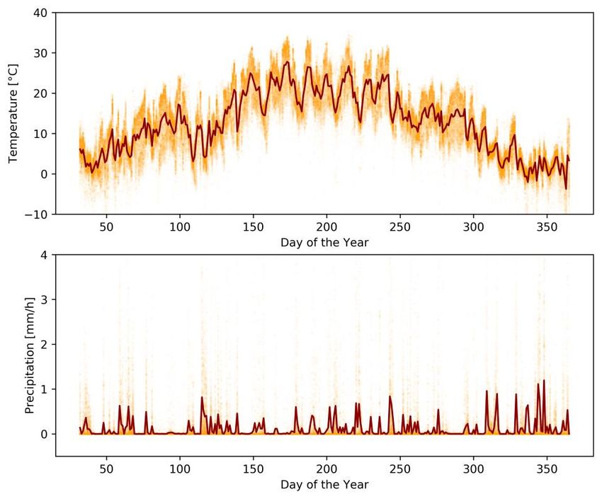
6 of 23

the distribution of tripleg transport modes on the left and the distribution of staypoint
purposes on the right. Out of all triplegs 122’063 were either covered by car (42’739;
35.0%) or e-car (79’324; 65.0%), which resulted in a total distance of 1’450’401 km by
car and 1’258’553 km by e-car.

The motivation of study participants usually decreases over time. This resulted in
study participants taking less care when validating the detected transport modes. In par-
ticular the distinction between car and e-car/EV is difficult from GPS data alone, which
is why a careful and trustworthy validation would be of essence. As we are unable to
force study participants to validate their input, we additionally use the data collected by
the EV itself for validation. This data includes the start and end locations of each drive
registered by the EV, with an associated change in kilometers and state of charge (SoC).
The matching of both datasets is tricky because both are subject to different spatio-
temporal uncertainties. We use the rule-based approach for the matching of app-record-
ing and EV-recording pairs described in [21]. This approach considers the spatio-tem-
poral distance between start and end points, the temporal overlap and the ratio of the
length of the app-tripleg and the difference in the km-counter of the EV. Afterwards,
we checked for consistency in sequences of trips, in order to ensure that impossible
combinations like driving to work by car and back by EV do not appear in the dataset.

In addition, we used weather data collected by the automatic weather monitoring
network of the Swiss Federal Office of Meteorology and Climatology MeteoSuisse1.
As this data is only available at certain measurement locations, it was interpolated spa-
tially and temporally following the method outlined in [4]. In essence, a temperature
correction coefficient that is dependent on the distance to the closest weather stations
as well as on the difference in elevation is computed and applied to every GPS posi-
tionfix for which a temperature measurement is required (usually the start of triplegs
and trips). From the automatic weather monitoring network, the temperature as well as
the precipitation were extracted, as these are generally the weather factors influencing
transport mode choice the most. Figure 2 shows the measurements at the beginning of
each tripleg as well as their average over the year.

Finally, the study participants were asked to fill in a range of surveys. Of particular
importance are the socio-demographic features recorded this way, a selection of which
is shown in Table 1. It is visible from this data that there is a bias towards male partic-
ipants with above average age and income. The demographic data corresponds to the
study participants, however, the car can theoretically be used by anyone in the house-
hold. As not all of the participants have both an electric and an ICE car, we removed 9
people who did not own a car at the time the study started, which resulted in 129 par-
ticipants whose data are used for the analysis presented below.

1
For information about the automatic weather monitoring network of MeteoSuisse consider
https://www.meteoschweiz.admin.ch/home/mess-und-prognosesysteme/bodenstationen/au-
tomatisches-messnetz.html.

7 of 23

Fig. 2. Temperature and precipitation at the start of each tripleg over the course of the one-year
study period as well as the average as bold line. The offset in the beginning results from a slightly
delayed start of the study and the fact that participants received their EV on different dates.

Table 1. Features taken from the socio-demographic survey and used within the models pre-
sented in this paper. Note that the median income is exactly CHF 17’500 as this variable was
measured as one of the following classes: {6’500, 10’000, 13’500, 17’500, 22’500}. *Number
of cars prior to receiving the EV. The 9 participants without cars are not considered in the other
distributions in the table.

 Feature Distribution
 Sex 111 male (86.0%)
 18 female (14.0%)
 Number of cars in household* 9 with 0 cars (6.5%)
 47 with 1 cars (34.1%)
 67 with 2 cars (48.6%)
 12 with 3 cars (8.7%)
 3 with 4 cars (2.2%)

AGILE: GIScience Series, 1, 2020.
Full paper Proceedings of the 23rd AGILE Conference on Geographic Information Science, 2020.
Editors: Panagiotis Partsinevelos, Phaedon Kyriakidis, and Marinos Kavouras
This contribution underwent peer review based on a full paper submission.
https://doi.org/10.5194/agile-giss-1-2-2020 | © Authors 2020. CC BY 4.0 License.

8 of 23

Work status 118 working full-time (91.5%)
10 working part-time (7.8%)
1 not working (0.8%)
Household size (no. of people) 11 with 1 person (8.5%)
36 with 2 persons (27.9%)
24 with 3 persons (18.6%)
33 with 4 persons (25.6%)
19 with 5 persons (14.7%)
6 with 6+ persons (4.7%)
Age 47.3 ± 7.6 years
Household income 16’791 ± CHF 4’358
(median CHF 17’500)
Total 129 eligible participants

4 Method

In our work, we analyze the users’ mobility choice behavior on two levels: The atomic
tripleg and the aggregated tour level. We choose to analyze the mobility behavior on
the tripleg level because it is the smallest unit in which we measure movement. How-
ever, it is likely that choices between taking the ICE car and the EV cannot be explained
solely on a tripleg level. This becomes clear if we look at the example of a user that
leaves home in the morning to go to work, goes shopping after work, and then returns
home. If such users choose to go to work using the EV, they will be forced to also take
the EV in the evening for their errands and the way home. Looking at complete tours
allows us to more closely follow the decision process of a user, who always has to take
the complete mobility chain until reaching the initial position again into account. Even
if both perspectives are different, we expect that there will be a large overlap between
the mode choice models on the tripleg level and the tour level model.

4.1 Data Preprocessing
Based on the staypoints and triplegs provided by the tracking app, we use a hierarchical
model of human mobility to extract trips (explained in Section 3) and tours. A tour is
defined as a closed loop in the daily mobility of a user. This means we add all triplegs
to the same tour that fulfill all of the following requirements:
 End respectively start less than 350 meters apart from each other.
 Were undertaken on the same day (± 12 hours).
 Are longer than 350 meters.

9 of 23

All tours that start and end at the user’s home location are called home-based tour or
journey. In general, it is possible for tours to contain sub-tours. An example for a typical
journey that contains a sub-tour is the following: A person wakes up at home, takes the
car to go to work, walks to a local grocery store during her break to buy snacks and
some groceries, then goes back to work and drives home after she is finished. Here, all
trips undertaken are part of the user’s journey and the trip to the supermarket and back
is a sub-tour. Our method is implemented such that also sub-tours are detected. For our
analysis, we consider all tours that contained either a minimum of one tripleg covered
by car or e-car and start and end at a user’s home (i.e., all journeys).

4.2 Outlier Removal and Downsampling of the Majority Class
As the dataset is from a smartphone-based tracking study it is subject to noise and un-
certainty. This can include sudden jumps, positions that are frozen over a longer period
of time or gaps. We filter these tracking-related outliers by excluding triplegs that have
an abnormally high average speed or abnormally low average speed2 and in a second
step, we fit a robust 2-dimensional normal distribution to the length-duration distribu-
tion of the triplegs and exclude the least-likely 3% of the data.

The final data after filtering includes 39’409 car triplegs, 73’388 e-car triplegs, 9’339
car tours and 24’550 e-car tours. To avoid bias when reporting results, we randomly
sample from the majority class without replacement such that the tour and tripleg da-
taset are class-balanced with respect to the transport mode (car or e-car). This leads to
a new dataset of 78’818 class-balanced triplegs and 18’678 class-balanced tours.

4.3 Feature Engineering and Extraction
To analyze the choice of a specific user, we test variables from three different catego-
ries: socio-demographic variables sourced from user surveys, tour respectively tripleg
descriptors recorded by the tracking app (and enhanced by the EV data) and spatio-
temporal context variables created by combining the available data with other environ-
mental datasets, most notably the temperature and precipitation.

Table 2 shows all the features that we used as predictors in the models for the tripleg
and the tour based approaches. As not all the data is available on the tour level (in
particular, only the aggregate of all triplegs can be considered when modeling mode
choice on a tour level), the predictors resp. models slightly differ. The features shown
in Table 2 are the features that were originally generated, however, many of them are
only marginally useful as predictors, and thus not always reported anymore. The tripleg
length is computed based on a map-matched geometry, i.e., all positionfixes making up

2
We consider an average speed of more than 220 km/h and less than 3 km/h as abnormal.

10 of 23

a tripleg were matched to the respective transport network using the map matching al-
gorithm available through the Open Source Routing Machine (OSRM) [18] 3. The pur-
pose of a trip is the next activity’s purpose, while the purpose of a tour is computed
using a majority vote on the purposes of all the staypoints visited during the tour. For
the spatio-temporal context, we always considered the starting time of the tripleg resp.
tour (e.g., the temperature is simply taken at the location and time of the first positionfix
of the respective tripleg or tour). The socio-demographic features were attached to each
tripleg resp. tour based on the user ID and used as independent variable similar to the
tripleg/tour descriptors and spatio-temporal context.

Table 2. The different features used for this study and the respective variable’s type. Nominal
variables are encoded as dummy variables, each denoting the presence of one of the labels. *For
tour-level analyses these features are not used. **Prior to the start of the study. ***Normalized
to lie in [0, 1].

 Feature Type Coding
 Tripleg/Tour descriptors
 Tripleg length* Ratio [0, ∞)
 Tripleg duration* Ratio [0, ∞)
 Length of all triplegs in tour cov- Ratio [0, ∞)
 ered either with car or e-car
 Tour length Ratio [0, ∞)
 Tour duration Ratio [0, ∞)
 Previous staypoint duration* Ratio [0, ∞)
 Next staypoint duration* Ratio [0, ∞)
 Purpose of trip* Nominal {home, work, errand, leisure,
 wait, unknown}
 Purpose of tour Nominal {home, work, errand, leisure,
 wait, unknown}
 Socio-demographic data
 Sex Nominal {male, female}
 Age Ratio [0, ∞)
 Cars in household** Ratio [0, ∞)
 Employment status Nominal {working, not working}
 Household income Ratio [0, ∞)

3
 The OSRM can be downloaded from http://project-osrm.org.

AGILE: GIScience Series, 1, 2020.
Full paper Proceedings of the 23rd AGILE Conference on Geographic Information Science, 2020.
Editors: Panagiotis Partsinevelos, Phaedon Kyriakidis, and Marinos Kavouras
This contribution underwent peer review based on a full paper submission.
https://doi.org/10.5194/agile-giss-1-2-2020 | © Authors 2020. CC BY 4.0 License.

11 of 23

Household size Ratio [0, ∞)
Spatio-temporal context
Hour of day*** Ordinal {0, 1, …, 23}
Weekday/weekend Nominal {weekday, weekend}
Month of year*** Ordinal {1, …, 12}
Temperature at start Interval [-273.15, ∞)
Precipitation at start Ratio [0, ∞)

Some of the values for the features were missing and were imputed using the median
of all available data for this variable. For triplegs, 4% (5’328) of the values for sex, age,
cars in household, employment status and household size (1 user), and 15% (17’209)
of the values for household income were missing. As the tours are based on the same
data, they show a similar pattern of missing data. Finally, all the nominal predictors
having more than two classes were encoded using dummy variables. This means that
instead of having one feature that denotes the purpose, we instead have six features that
indicate if the purpose was one of the given six categories in a binary fashion (one-hot
encoding).

4.4 Modeling E-Car Choice
To determine the suitability of the introduced features for predicting the mode choice,
we run the following 4 experiments for the tripleg and the tour level.

Random Forest Model. In the first experiment, we fit a random forest (RF) classifier
on all features to predict the choice of all users. RFs are a class of ensemble models that
combine several decision trees with random feature selection on bootstrapped samples
(a variation of bagging with decision trees). RFs were introduced in [3] and are robust
against overfitting and require little hyperparameter tuning. A RF is a non-linear clas-
sifier that usually performs close to the state-of-the-art on tabular data for regression
and classification problems. However, while the visualization of decision boundaries
and the variable importance offer some degree of explainability for RF-models, it is
hard to understand the exact relationship between inputs and the target. We therefore
use the RF model to create an upper-boundary baseline for the accuracy and fit logistic
regression based mode-choice models for interpretation.

Logit Model. To get a better and more interpretable understanding of the relationship
between input variables and the decision of the user to take the ICE car or the EV, we
fit a logarithmic regression model (logit). Logits are the widely accepted standard in
transport planning for mode-choice models (cf. [9]), especially because of their capa-
bility to work with mixed integer and continuous input variables and their interpreta-
bility. However, due to their linear nature, all non-linear and all cross-relations between

12 of 23

inputs and the target have to be precalculated explicitly. We define the logistic regres-
sion model that predicts the probability of the target variable being 1 as
 1
 ( ) = 
 (1)
 1 + − 
where is the ith vector of observations and β are the weights of the model. We fur-
thermore define the logistic per-sample loss as

 = − log( ( )) − (1 − ) log(1 − ( )) (2)

where is the true binary label associated with the ith observation. We identify the
parameters β by minimizing the following regularized total loss function
 
 = ∑ ( , ) + ∑ 2 (3)
 =1 =1

where α is a tuneable hyperparamter, n is the number of data points, is the jth model
parameter and m is the number of model parameters. The predictions ( ) are used
to create the following classifier:
 0 ( ) < 0.5
 ( ) = { (4)
 1 ( ) ≥ 0.5

To make up for the linearity of the logit model, we manually transform some features
based on their histograms. In particular, if a feature shows a periodic pattern (e.g., the
temperature over the course of a year) or follows a power law (e.g., the distance trav-
elled), we apply a trigonometric resp. a logarithmic function. The resulting transformed
features are directly used as input for the logit model.

User Specific Models. In the final experiment, we want to investigate the generaliza-
tion properties of the random forest and the logit models for the given problem. We
refit the same RF and logit models but use a user-specific data split for the cross-vali-
dation scheme.

 This means that the set of users in the training data and the set of users in the test
data are disjunct. This test allows us to analyze if the random forest model could actu-
ally identify underlying user-independent rules that explain under which circumstances
people prefer to take an EV or an ICE car. If the random forest fails to generalize in
this experiment, it indicates that it simply remembers user-specific patterns and prefer-
ences.

4.5 Model Performance Metrics
We use two metrics to evaluate the performance of the proposed models: Accuracy and
 2. Accuracy is a widely accepted and easy to interpret classification metric that is
defined as

AGILE: GIScience Series, 1, 2020.
Full paper Proceedings of the 23rd AGILE Conference on Geographic Information Science, 2020.
Editors: Panagiotis Partsinevelos, Phaedon Kyriakidis, and Marinos Kavouras
This contribution underwent peer review based on a full paper submission.
https://doi.org/10.5194/agile-giss-1-2-2020 | © Authors 2020. CC BY 4.0 License.

13 of 23

= (5)
+
where and are the counts of correctly and incorrectly classified sam-
ples, respectively. Accuracy is very easy to interpret but it is misleading if class counts
in the sample are unbalanced. As we operate in a binary classification regime, 50%
accuracy corresponds to random guessing.

As a second metric, we report the McFadden (pseudo) 2 introduced in [23]. This
score represents an alternative to the well-known 2 score which is not meaningful for
binary classification tasks. The McFadden pseudo 2 is defined as

2
ln 1
= 1− (6)
ln 0
where 0 is the likelihood of the null model (a model only fitted with the intercept) and
1 is the likelihood of the controlled model. As the logarithm of the likelihood is always
negative, the log-likelihood of a good model goes towards 0 and because 0 is constant,
this drives the McFadden score towards 1. The other way around, if the analyzed
model’s log-likelihood is similar to the one of the null model (this means without great
explanatory value), then the McFadden pseudo 2 score goes towards 0. While this
behavior is similar to the regular 2, the values of the McFadden pseudo 2 are usually
significantly lower, such that a score above 0.2 is already considered good [22]. We
calculate the McFadden pseudo 2 score according to Equation 6 using a logit model
only containing an intercept as the null model. This means the fitted model is able to
only predict a single constant for all samples. The logit model is fitted without any
regularization and using the Limited-memory BFGS (cf. [20]) solver.

5 Results

In the following, we describe the fitting of the final models used for each of the exper-
iments and report their accuracy, pseudo 2 and the significance and importance of
various predictors. Furthermore, we will quickly elaborate on the most important take-
aways for each model. A comparative discussion of the different models and the impli-
cations on the mode choice problem is given in Section 6. All the data preprocessing
and all the models were implemented in Python using the scikit-learn [26] (for the ran-
dom forests) and statsmodels [29] (for the logistic regression) libraries.

5.1 Random Forest Models
The random forest baselines for the tour and the tripleg level experiment simply use all
features introduced above to predict the binary outcome {car, e-car}. For both models,
we chose 1000 trees, the Gini impurity as quality criterion, the square root of the total
number of features as the number of features per split and an unrestricted tree depth as
hyperparameters. The data was randomly split according to a 3:1 proportion; while the

14 of 23

first 75% were used to train the RF, the remaining 25% were used to compute the ac-
curacy of the prediction (cf. Section 4.5).

Table 3. Accuracies and pseudo 2 for the models used within this paper.

Model Accuracy Pseudo R2
Random Forest Triplegs 78.86% 0.3060
Random Forest Tours 74.04% 0.2198
Logit Triplegs 59.00% 0.0195
Logit Tours 58.46% 0.0328
Random Forest Triplegs (User Split) 65.40% 0.1032
Random Forest Tours (User Split) 59.96% 0.0273
Logit Triplegs (User Split) 57.28% 0.0055
Logit Tours (User Split) 52.43% -0.0072

Table 3 shows the values for accuracy and the pseudo 2 for the different models. Fig-
ure 3 contains the same information, visualized for a more immediate comparison of
the models. The baseline RF reaches an accuracy of 78.86% on the tripleg level, and
74.04% on the tour level, indicating that it is feasible to predict if someone chooses the
ICE car or the e-car. Similarly, the high pseudo 2 values of 0.3060 resp. 0.2198 indi-
cate that the predictors (in their aggregation) are able to explain the variance in transport
mode choice well.

Fig. 3. Accuracies vs. pseudo 2 and feature importances of all the models evaluated within this
work.

15 of 23

5.2 Linear Logistic Regression Models
To have a more readily interpretable model, we fitted a logit model (only considering
linear superpositions) between the features and the discrete target. The here presented
models for triplegs and tours are the result of both a manual search for a model that
balances explainability and prediction ability as well as an automated model finding
process.

Mode Choice on a Tripleg Level. Table 4 shows the chosen predictors for the logit
model on the tripleg level, and their model parameters and significances. The omitted
predictors (compared to all the features displayed in Table 2) were either not significant
given the training data, or did not substantially add to the model. It can be seen that the
presence of the long-distance marker (triplegs longer than 100 km) strongly drives the
choice, as do the distance and duration related predictors as well as the weekday/week-
end marker. Note that since the models are not normalized (except the hour of day and
month of year features, cf. Table 2), the coefficients cannot be directly used to compare
the importance of different predictors. However, having these non-normalized coeffi-
cients allows for example comparing the influence of the difference in 1° Celsius with
a distance increase of 10 km. From the model, it can be seen that the weather context is
only minimally important, as is the age, household size and hour of day.

Table 4. Model parameters and predictor significances for the tripleg logit model. *Significant
at the p < 0.05 level.

Feature Coefficient Std. Error z-Value p-Value
Intercept 3.7693 0.310 12.175 0.000*
Weekday/weekend -0.4806 0.017 -27.879 0.000*
Temperature 0.0078 0.001 7.719 0.000*
Precipitation 0.0394 0.012 3.244 0.001*
Sex -0.1872 0.025 -7.638 0.000*
Age 0.0086 0.001 8.037 0.000*
Numbers of cars in household -0.0636 0.012 -5.425 0.000*
Work status 0.3381 0.023 14.635 0.000*
Household size 0.0689 0.006 11.811 0.000*
Long-distance tripleg -1.7695 0.064 -27.848 0.000*
log(duration of next activity) 0.0776 0.005 14.868 0.000*
log(duration of prev. activity) 0.0852 0.005 15.984 0.000*
log(duration of tripleg) -0.3136 0.018 -17.038 0.000*
log(length of tripleg) 0.2011 0.014 14.614 0.000*

16 of 23

log(household income) -0.4286 0.031 -14.023 0.000*
sin(hour of day) 0.0928 0.011 8.359 0.000*
sin(month of year) 0.2385 0.011 21.001 0.000*

The logit model is greatly outperformed by the corresponding random forest. With an
accuracy of 59% and significantly lower pseudo 2 values the logit model is clearly the
less powerful model. This is an indication that many of the relations that the RF model
learned from the randomly split data are non-linear and not included in our self-gener-
ated more obvious set of non-linear features.

Mode Choice on a Tour Level. Looking at the logit model on the tour level (shown in
Table 5), we see a similar distribution of predictor coefficients. Again, the presence of
the long-distance marker has a substantial influence, just as the other distance-related
predictors do. It seems that the overall length of the tour is a more important criterion
than the parts covered by car resp. e-car. Again, and also indicated by the p-values,
there is no significant relation between contextual factors such as the temperature, pre-
cipitation, or household characteristics. It needs to be noted that the interpretation of
the impact of sex and work status on the mode choice is difficult as there is a large bias
towards working males in our dataset. The accuracy of the model similarly drops to
around 58.5%, with a corresponding 2 score of 0.0328, indicating that the model is of
lower explanatory power than the corresponding random forest model.

Table 5. Model parameters and predictor significances for the tour logit model. *Significant at
the p < 0.05 level.

Feature Coefficient Std. Error z-Value p-Value
Intercept -1.7069 0.611 -2.792 0.005*
Weekday/weekend -0.4440 0.035 -12.632 0.000*
Temperature -0.0018 0.002 -0.850 0.395
Precipitation -0.0357 0.029 -1.238 0.216
Sex -0.1451 0.049 -2.975 0.003*
Age 0.0078 0.002 3.503 0.000*
Numbers of cars in household -0.0250 0.024 -1.030 0.303
Work status 0.6985 0.260 2.689 0.007*
Household size 0.0900 0.012 7.509 0.000*
Long-distance tour -0.5116 0.053 -9.670 0.000*
log(length of all triplegs by car 0.0464 0.009 5.206 0.000*
or e-car)

17 of 23

log(length of tour) 0.1006 0.020 5.066 0.000*
log(duration of tour) 0.0620 0.017 3.704 0.000*
log(household income) -0.0584 0.062 -0.940 0.347
sin(hour of day) 0.1443 0.024 6.043 0.000*
sin(month of year) 0.1223 0.023 5.282 0.000*

5.3 Random Forest - User Split
As random forests are very robust non-linear models, they are prone to learn “hidden”
connections in the data that lead to non-generalizable results. To test for these effects,
we here present the results from applying the same RF model to the tripleg and tour
data, but restricting training to a subset of users, and testing on another.

Looking at the reported values in Table 3 (comparing the entries for Random Forest
and Random Forest (User Split)), it is easily visible that the RF model does not gener-
alize well across users. Making predictions about unknown users lets the accuracy of
the random forest drop by about 15% in both cases. The pseudo 2 shows a similar
decrease, meaning that the explanatory value of the user-independent model drops sig-
nificantly. Considering that a random prediction would already yield an accuracy of
50% in the given case, the resulting accuracy of about 60% is only a slight improve-
ment. This performance drop is evidence that the random forest trained using a random
data split is remembering the users’ decisions instead of identifying underlying general
rules.

Fig. 4. Feature importances in the random forest model including a user split. On the left side,
the importances for the tripleg model are shown, on the right side the ones for the tour model.

Figure 4 shows the feature importances extracted from the RF model. Similar to the
logit models, the length and duration features are most important for the mode choice.
This shows that the same features can be used to identify (weak) generalizable rules as
well as identifying the user’s unique (e.g., non-generalizable) mobility behavior.

18 of 23

5.4 Linear Logistic Regression Models - User Split
Finally, we included the results of a logistic regression model trained on a subset of
users and evaluated (for accuracy) on another subset of users. As expected, the results
in Table 3 show that the original logit model already generalizes well, but thus also has
a substantially lower explanatory power. We do not report the complete models here,
as they do not substantially differ from the ones in Tables 4 and 5.

6 Discussion and Conclusion

Driven by goals of sustainability, related monetary incentives and technological ad-
vances, people buying a new car today have to decide between an electric vehicle and
a regular internal combustion engine car. For many, this poses a difficult decision as
they are usually not aware of how the limited range, refueling capacity and differing
storage and driving characteristics might influence their future driving behavior. Using
a unique constellation of people that have both types of cars at their service and have
to take the decision whether to take the EV or the ICE car every day, we try to give
insight into the decision process that leads to people choosing one type of car over the
other. We analyze data from 129 ICE car and EV owners of a real-life study (involving
138 participants in total) that were tracked over the duration of a year via an app on
their phone and via the EV itself. The chosen measures of interest are the accuracy in
predicting the transport mode of previously unseen triplegs and tours and the 2 which
summarizes the explanatory power of the models. To have both a well-performing up-
per bound as well as more easily interpretable models, we fit random forests and logit
models to features extracted from the raw data. These features are chosen with respect
to the uncertainties related to EVs, namely the distance and duration of trips, the
weather, personal background, and more.

Looking at the presented results in detail, there are several interesting takeaways.
Even though all models are better than a random guess, their predictive power is com-
parably low. Only the random forest that is trained on data from all the users manages
to reach both a high accuracy as well as a high 2 score. This is a strong indication that
the random forest simply learns to identify individual users by unique combinations of
features, and thus also that for each user individually most mode choices follow a sys-
tematic pattern (resp. on the same trips, e.g., going to work, a single user will in most
cases choose the same mode of transport). Training the models on a subset of people
confirms the hypothesis that the logit models generalize as well as can be expected,
namely in a similar range as the random forests on the user-split data. Looking at the
predictors, we can see that the distance and duration, but also if the tripleg or tour took
place on the weekend influence the choice more than factors such as the household size
or age of the participant. However, contrary to our initial assumption and hypothesis,
all predictors are of a weak nature, i.e., while they manage to positively influence the
predictions, the resulting accuracies are still only slightly better than a random guess.
A potential reason for this might be that the choice between ICE car and EV is mainly
driven by variables not measured as part of the study: the size of the cars (which we

19 of 23

only know for the EV), the number of people participating in a trip, the necessities of
other household members, or the overall distribution of work and household duties
within a family. Clustering people into groups based on these variables, or also based
on the number of cars or people in a household could reduce the variability in the (sub-
)datasets, thus increasing the predictive power of the presented models and explain bet-
ter why someone chooses the ICE car or EV in a given situation. It is similarly inter-
esting that the prediction of the transport mode choice for individual triplegs seems
easier than for complete tours. We suspect that this is due to the fact that there are more
triplegs that appear in a very similar fashion in the dataset (e.g., a single home-work-
home tour results in two triplegs that exhibit almost the same characteristics: one from
home to work, and another one back). As such, we have to consider the lower predictive
power of the tour level models as a “realistic” view on how a person would choose the
transport mode in a real situation.

Comparing our research to previous studies, it is in line considering the importance
of individual features. However, our findings of comparatively low predictive power of
the different models indicate that looking at a general population, their choices are not
easily predictable and are determined by features that cannot be captured by GPS track-
ing or simple socio-demographic surveys alone. Considering all this, our work provides
an addition to the scarce literature on car and e-car choice models, but should be ex-
tended with more in-depth analyses of additional transport mode choice predictors in
the future. Similarly, our focus was limited to choice predictions based on individual
data: Future work should capture the complexity of mobility choices in a more holistic
way, e.g., by closely observing other household members as well. For individual driv-
ers, it seems that they will not have to worry too much about the limited range or charg-
ing infrastructure, though, as the choice for one mode or the other is only marginally
explained by the distance covered.

Acknowledgements

This research was supported by the Swiss Data Science Center (SDSC) and by the
Swiss Innovation Agency Innosuisse within the Swiss Competence Center for Energy
Research (SCCER) Mobility.

Bibliography

[1] Kristin Ystmark Bjerkan, Tom E Nørbech, and Marianne Elvsaas Nordtømme. In-
centives for promoting battery electric vehicle (bev) adoption in norway. Transporta-
tion Research Part D: Transport and Environment, 43:169–180, 2016.

[2] Lars Böcker, Patrick van Amen, and Marco Helbich. Elderly travel frequencies and
transport mode choices in greater rotterdam, the netherlands. Transportation,
44(4):831–852, 2017.

20 of 23

[3] Leo Breiman. Random Forests. Machine Learning, 45(1):5–32, October 2001.

[4] Dominik Bucher, René Buffat, Andreas Froemelt, and Martin Raubal. Energy and
greenhouse gas emission reduction potentials resulting from different commuter elec-
tric bicycle adoption scenarios in switzerland. Renewable and Sustainable Energy Re-
views, 114:109298, 2019.

[5] Ralph Buehler. Determinants of transport mode choice: a comparison of germany
and the usa. Journal of transport geography, 19(4):644–657, 2011.

[6] Naznin Sultana Daisy, Hugh Millward, and Lei Liu. Trip chaining and tour mode
choice of non-workers grouped by daily activity patterns. Journal of Transport Geog-
raphy, 69:150–162, 2018.

[7] Thomas Franke and Josef F Krems. Interacting with limited mobility re-sources:
Psychological range levels in electric vehicle use. Transportation Research Part A: Pol-
icy and Practice, 48:109–122, 2013.

[8] Edgar G Hertwich and Glen P Peters. Carbon footprint of nations: A global, trade-
linked analysis. Environmental science & technology, 43(16):6414–6420, 2009.

[9] Stephane Hess. Advanced discrete choice models with applications to transport de-
mand. PhD thesis, University of London, 2005.

[10] Anders F. Jensen and Stefan L. Mabit. Modelling Real Choices Between Conven-
tional and Electric Cars for Home-based Journeys. In The 14th International Confer-
ence on Travel Behaviour Research (IATBR), pages19–23, 2015.

[11] Anders Fjendbo Jensen, Thomas Kjær Rasmussen, and Carlo Giacomo Prato. A
Joint Route Choice Model for Electric and Conventional Car Users. In International
Choice Modeling Conference (ICMC), 2017.

[12] George Kamiya, Jonn Axsen, and Curran Crawford. Modeling the ghg emissions
intensity of plug-in electric vehicles using short-term and long-term perspectives.
Transportation Research Part D: Transport and Environment, 69:209–223, 2019.

[13] Christian Andreas Klöckner, Alim Nayum, and Mehmet Mehmetoglu. Positive and
negative spillover effects from electric car purchase to car use. Transportation Research
Part D: Transport and Environment, 21:32–38,2013.

[14] Philippe Lebeau, Cathy Macharis, and Joeri Van Mierlo. Exploring the choice of
battery electric vehicles in city logistics: A conjoint-based choice analysis. Transporta-
tion Research Part E: Logistics and Transportation Review, 91:245–258, 2016.

21 of 23

[15] Dongwoo Lee, Sybil Derrible, and Francisco Camara Pereira. Comparison of four
types of artificial neural network and a multinomial logitmodel for travel mode choice
modeling. Transportation Research Record, 2672(49):101–112, 2018.

[16] Fangyi Li, Bofeng Cai, Zhaoyang Ye, Zheng Wang, Wei Zhang, Pan Zhou, and
Jian Chen. Changing patterns and determinants of transportation carbon emissions in
chinese cities. Energy, 174:562–575, 2019.

[17] Chengxi Liu, Yusak O Susilo, and Anders Karlström. The influence of weather
characteristics variability on individual’s travel mode choice in different seasons and
regions in sweden. Transport Policy, 41:147–158, 2015.

[18] Dennis Luxen and Christian Vetter. Real-time routing with openstreetmap data. In
Proceedings of the 19th ACM SIGSPATIAL International Conference on Advances in
Geographic Information Systems, GIS ’11, pages 513–516, New York, NY, USA,
2011. ACM.

[19] Jennifer MacDonald. Electric vehicles to be 35% of global new car sales by 2040.
Bloomberg New Energy Finance, 25, 2016.

[20] Robert Malouf. A comparison of algorithms for maximum entropy parameter es-
timation. In proceedings of the 6th conference on Natural language learning - Volume
20, pages 1–7. Association for Computational Linguistics, 2002.

[21] Henry Martin, Henrik Becker, Dominik Bucher, David Jonietz, Martin Raubal,
and Kay W Axhausen. Begleitstudie sbb green class - abschlussbericht. Arbeitsberichte
Verkehrs- und Raumplanung, 1439, 2019.

[22] D McFadden. Quantitative methods for analyzing travel behaviour of individuals:
Some recent developments (cowles foundation discussion papers no. 474). Cowles
Foundation for Research in Economics, Yale University, 1977.

[23] Daniel McFadden et al. Conditional logit analysis of qualitative choice behavior.
1973.

[24] Marcel Paulssen, Dirk Temme, Akshay Vij, and Joan L Walker. Values, attitudes
and travel behavior: a hierarchical latent variable mixed logit model of travel mode
choice. Transportation, 41(4):873–888, 2014.

[25] Nathaniel S Pearre, Willett Kempton, Randall L Guensler, and Vetri VElango.
Electric vehicles: How much range is required for a day’s driving? Transportation Re-
search Part C: Emerging Technologies, 19(6):1171–1184, 2011.

You can also read