Estimation of Moran's I in the Context of Uncertain Mobile Sensor Measurements - Schloss ...
←
→
Page content transcription
If your browser does not render page correctly, please read the page content below
Estimation of Moran’s I in the Context of
Uncertain Mobile Sensor Measurements
Dominik Bucher1
Institute of Cartography and Geoinformation, ETH Zurich, Switzerland
dobucher@ethz.ch
Henry Martin1
Institute of Cartography and Geoinformation, ETH Zurich, Switzerland
martinhe@ethz.ch
David Jonietz
HERE Technologies Switzerland, Zurich, Switzerland
david.jonietz@here.com
Martin Raubal
Institute of Cartography and Geoinformation, ETH Zurich, Switzerland
mraubal@ethz.ch
René Westerholt1
School of Spatial Planning, TU Dortmund University, Germany
rene.westerholt@tu-dortmund.de

        Abstract
Measures of spatial autocorrelation like Moran’s I do not take into account information about the
reliability of observations. In a context of mobile sensors, however, this is an important aspect to
consider. Mobile sensors record data asynchronously and capture different contexts, which leads to
considerable heterogeneity. In this paper we propose two different ways to integrate the reliability
of observations with Moran’s I. These proposals are tested in the light of two case studies, one
based on real temperatures and movement data and the other using synthetic data. The results
show that the way reliability information is incorporated into the Moran’s I estimates has a strong
impact on how the measure responds to volatile available information. It is shown that absolute
reliability information is much less powerful in addressing the problem of differing contexts than
relative concepts that give more weight to more reliable observations, regardless of the general degree
of uncertainty. The results presented are seen as an important stimulus for the discourse on spatial
autocorrelation measures in the light of uncertainties.
2012 ACM Subject Classification Information systems → Geographic information systems; Inform-
ation systems → Sensor networks; Mathematics of computing → Statistical paradigms; Applied
computing → Earth and atmospheric sciences
Keywords and phrases mobile sensors, Moran’s I, uncertainty, probabilistic forecasting
Digital Object Identifier 10.4230/LIPIcs.GIScience.2021.I.2

Funding This research was supported by the Swiss Data Science Center (SDSC) and by the Swiss
Innovation Agency Innosuisse within the Swiss Competence Center for Energy Research (SCCER)
Mobility.

    1    Introduction
Recent technological advances accompanied by price reductions of sensor hardware have
propelled the emergence of mobile sensor networks. Mobile sensor data is widely collected
using smartphones [27, 56], sensor-equipped cars and public transport vehicles [31, 28],
boats [2], animals [52], or semi-stationary objects like buoys [33]. Such mobile sensors make

1
    These authors contributed equally to this work.
            © Dominik Bucher, Henry Martin, David Jonietz, Martin Raubal, and René Westerholt;
            licensed under Creative Commons License CC-BY
11th International Conference on Geographic Information Science (GIScience 2021) – Part I.
Editors: Krzysztof Janowicz and Judith A. Verstegen; Article No. 2; pp. 2:1–2:15
                   Leibniz International Proceedings in Informatics
                   Schloss Dagstuhl – Leibniz-Zentrum für Informatik, Dagstuhl Publishing, Germany
2:2 Moran’s I in the Context of Uncertain Mobile Sensor Measurements
it possible to increase the spatial coverage of data collection while deploying relatively few
additional devices compared to static sensor networks [15, 44]. Mobile sensors hence allow
monitoring of our social and physical environments at a so far unprecedented scale.
Increasing the spatial coverage of sensor networks using mobile instead of static devices
can entail a loss of homogeneity in the collected data. Mobile measurements are often
recorded at different locations, at different points in time, and in an asynchronous mode.
They thus capture differing contextual conditions [38]. Mobile sensor data therefore may
represent different processes of dynamic geographic phenomena. For instance, measuring
air temperature at different times of the day may result in collecting samples representative
of different processes such as urban heating at midday or cooling at night due to atmo-
spheric radiation losses into outer space. Such processes may behave very differently in
varying geographic regions despite involving the same phenomenon. Respective sensed data
may therefore be characterised by differing mean levels, dispersal mechanisms, and spatial
structures.
The outlined variations can distort the interpretation of measures and statistics obtained
from mobile sensor data. One example for this is the assessment of spatial autocorrelation,
which can be described as the quantification of spatial interaction, or as the “coincidence of
value similarity with locational similarity” [4, p. 241]. Computing the popular Moran’s I
index [43], for instance, establishes a relation between geographically close observations.
The statistic is thus highly sensitive to asynchronously sensed value pairs attached with
uncertainty, in particular when no or little prior knowledge is available about the underlying
processes. Novel ways are thus needed to incorporate this kind of uncertainty attached to
sensor measurements in the estimation of spatial measures.
This paper puts forward two approaches for estimating Moran’s I using uncertain mobile
measurements. Both approaches presented make use of weights reflecting the certainty
attached to pairs of sensor measurements. The certainty measures used are calculated
through a non-parametric probabilistic forecast of the measured values, with the underlying
model being constantly refitted from incoming sensor data. The certainty factors obtained
this way are then included in Moran’s I through two different kinds of matrices of pair-wise
terms, which rescale the spatial weights used in the statistic. The advantages of using
empirical forecasts to quantify uncertainty are that the temporal correlation does not have
to be modeled explicitly, that it allows treating problems that do not fall into a geostatistical
category (where we could model the spatio-temporal dependencies explicitly) and that it
naturally captures both uncertainties arising from the measured phenomenon itself as well as
from the sensors in use. We evaluate our concepts by applying them to two case studies: One
study contains data from sensor-equipped cars measuring air temperature in Switzerland
over a three day period, whereas the second one is based on controlled, synthetic data. The
latter study is used to investigate the capacity of our introduced certainty matrices to also
outweigh non-stationarity, that is, a temporally varying spatial process.
2 Related Work
2.1 Spatial Non-Stationarity
One characteristic causing uncertainty is spatial non-stationarity. This may be reflected in
variation in the mean, the variance, or higher-order moments. Ord & Getis have recently put
forward a measure called Local Spatial Heteroscedasticity (LOSH) [48, 72, 22]. It quantifies
spatially inhomogeneous variation allowing to disclose spatial boundaries separating regimes
and to characterise the internal stability of clusters [1]. Westerholt et al. [68] have modified
LOSH towards an entirely local test for identifying the role of spatial structure in local variance
characterisations. Varying mean levels are commonly investigated using residuals aboveD. Bucher, H. Martin, D. Jonietz, M. Raubal, and R. Westerholt 2:3
trend surfaces [7, 25], defining the mean as a function of the coordinates levelling out spatial
trends. Some kinds of data lead to non-stationarity, for instance, through uncontrolled data
acquisition procedures. One example for this is georeferenced social media data. Such data
are prone to uncertainty because people contribute in different ways simultaneously, including
varying cognitive (e.g., [54, 66]), demographic (e.g., [65, 57]), idiosyncratically subjective
(e.g., [12, 29]), and other factors pertaining to spatial perception and communication. Recent
works have investigated the impact of this uncontrolled uncertainty on the estimation of
spatial structure, and initial proposals were made to address related issues [69, 70, 67].
2.2 Spatiotemporal Autocorrelation
Uncertainty can enter estimations temporally, for example, when phenomena are not stable
over time. The notion of spatial autocorrelation is a way to address this issue. One
way to achieve this is to incorporate explicitly temporal notions of autocorrelation in the
calculation of spatial measures. First discussed by [11] and [41], various approaches to measure
spatiotemporal autocorrelation have been proposed, such as [37], who incorporate temporal
trends through time-lagged correlation measures into the calculation of Moran’s I. Another
approach is to estimate Moran’s I using spatiotemporal weight matrices, with exemplary
studies including [16], who focus explicitly on how to build such matrices; [30], who, focusing
on the related concept of geographically weighted regression (GWR), construct weight
matrices from spatiotemporal (x, y, t)-coordinates; and [35], who, based on the assumption
that spatiotemporal effects can be calculated as a product of spatial and temporal effects,
integrate the according weights in a combined matrix, and compute both global and local
spatiotemporal Moran’s I. A slightly different approach is taken by [53], whose approach
eliminates certain time effects by temporally detrending spatially referenced time series.
2.3 Investigation of Rates
Rate variables are commonly attached with varying uncertainty levels. This is caused
by varying underlying populations like populations at risk or varying numbers of people
counted in aggregation units [63, 64]. Rates have a higher propensity of being extreme
when the underlying reference quantity is small [5]. In order to correct for these distortions,
several approaches have been proposed including empirical Bayes correction [17, 40, 5, 32],
omission of local population sizes by re-basing rates on the overall population size [46], and
weighting deviations of residual rates by the inverse of the size of the local population at
risk [62]. Methodically, our approach proposed below is closest to the adjustment proposed
by Waldhör [62], but we focus on a different kind of uncertainty in this paper.
3 Methodology
3.1 Assumptions
Our work presented below is based on certain assumptions concerning our uncertainty
assessment and the spatial method Moran’s I that we modify. Let oil and ojm be elements of
a set of observations O of a spatial phenomenon Q taken at geographic locations i and j, and
at different points in time tl and tm , respectively. The following assumptions are assumed to
hold true for the remainder:
Observations O obtained from mobile sensors provide an incomplete representation of
the phenomenon Q studied.
A higher spatial coverage of observations O of Q can lead to an improved representation
of Q, even if taken at different points in time.
GIScience 20212:4 Moran’s I in the Context of Uncertain Mobile Sensor Measurements
The certainty uoil ,ojm shared between two observations depends on the forecast horizon
∆tlm comprising a certain number of preceding observations. Predictions of the nearer
future are considered more certain than distant ones.
Phenomenon Q is assumed to show relatively stable spatial second-order characteristics
over the time points observed. This facilitates meaningful interpretation of Moran’s I.
Although Q is geostatistical in the case study example, our proposed solution is free
of model assumptions to ensure transferability to social science domains such as social
media analysis or georeferenced surveys [6, 55].
3.2 Spatial Autocorrelation and Moran’s I
Tobler’s first law of geography states that “everything is related to everything else, but near
things are more related than distant things” [60, p. 234]. This characteristic can be utilised
for spatial interpolation, to detect pockets of non-stationarity, or to characterise spatial
heterogeneity [19]. Spatial autocorrelation operationalises this empirical law [42] to quantify
spatial associations [21] disclosing spatially clustered (positive), dispersed (negative), or
random behaviour (close to zero autocorrelation) [21]. A number of global and local measures
of spatial autocorrelation are available, including Moran’s I [43, 10, 3], Geary’s c [18, 3],
Rogerson’s R [50], and Getis and Ord’s G hotspot statistics [47, 23].
Moran’s I is often preferred over other measures because of its superior statistical power
properties and its robustness against unfavourable configurations of spatial units, that is,
outliers in the spatial weights matrix [9, 21]. Let xi be measured values with arithmetic
mean x̄. Moran’s I and its feasible range are then given as
n
wij (xi − x̄)(xj − x̄)
P
n i,j6=i n n
I= P . (1)
n · n , I∈ n · λmin , n · λmax
(xi − x̄)2
P P P
wij wij wij
i,j6=i i i,j6=i i,j6=i
Matrix W holds spatial weights wij . These establish pairwise connections between the n
spatial units based on their inverse distance, spatial contiguity, or other characteristics [20].
The measure strongly depends on the spatial weights structure chosen [13, 59]. Therefore,
the range of I depends on the smallest and largest eigenvalues λmin and λmax of the centred
symmetric part of the spatial weights matrix given as (I − 11T /n)((1/2)(W + W T ))(I −
11T /n). Thereby, I is the n × n identity matrix and 1 denotes the n × 1 all-ones vector.
Values of global Moran’s I below its expected value E[I] = −1/(n − 1) indicate negative
spatial autocorrelation. Values for I larger than E[I] hint on the opposite case [43, 10].
We argue that the effects of observations oil and ojm made at different points in time of a
temporally non-static phenomenon Q should be explicitly considered in the calculation of the
global Moran’s I. Our approach consists of extending traditional Moran’s I with measures of
pair-wise certainty uoil ,ojm (abbreviated to uil,jm hereafter), which represent the influence of
past time intervals on the reliability of measurements. The measures of certainty that we
use are equivalent to projecting values observed at time tl to more recent points in time tm ,
and hence to their hypothetical re-measurement. We propose two different ways to include
pair-wise certainty measures in Moran’s I. Let ∆tlm denote a temporal forecast horizon. The
indicators proposed are then given as
n
wil,jm uil,jm (oil − ō)(ojm − ō)
P
n i,j6=i
1
I∆tlm
= P
n · n , (2)
(oi − ō)2
P
wil,jm uil,jm
i,j6=i iD. Bucher, H. Martin, D. Jonietz, M. Raubal, and R. Westerholt 2:5
n
wil,jm (1 + uil,jm − ū)(oil − ō)(ojm − ō)
P
n i,j6=i
2
I∆t lm
= P
n · n . (3)
wil,jm (1 + uil,jm − ū) (oi − ō)2
P
i,j6=i i
In the indicator proposed in Equation 2 the spatial weights are rescaled proportional to the
joint certainties shared by neighboured locations. In practice, most weights will be affected,
but some weights more than others depending on their joint certainty. The terms uil,jm range
in the interval [0, 1]. Indicator I∆t
1
lm
equals standard Moran’s I only when no uncertainty is
present. In all other cases, I∆tlm shall be interpreted in the light of its feasible range given
1
in Equation 1 but with the eigenvalues of W substituted by those of the Hadamard product
Pn
W ◦ U and with the normalising factor replaced with n( i,j6=i wij uil,jm )−1 .
The second indicator defined in Equation 3 presumes that uncertainty is acceptable
as long as it is distributed evenly across the map. Whenever the joint certainty of two
observations is above average, their relative importance in the spatial analysis increases.
Analogously, when the mutual certainty of a pair of observations is below average, their joint
spatial weight is penalised. The terms 1 + (uil,jm − ū), with ū being the mean certainty
estimate, range in the interval [0, 2]. I∆t
2
lm
equates to Moran’s I when either all certainties
are close to their own average, or when there is at least a balance between above and below
average certainties in the map. Like with I∆t 1
lm
, we shall consider the respective eigenvalue
spectrum determining the feasible range of I∆t 2
lm
to assess the impact of the uncertainty
modelling proposed on the range of Moran’s I values.
3.3 Uncertainty Estimation using Empirical Prediction Intervals
We make use of the quantiles of empirical prediction intervals. Such intervals are a form
of probabilistic forecasting, expressing predictions of the future in the form of probability
distributions over all possible outcomes [24]. Empirical prediction intervals thus allow to
assign a degree of certainty (or uncertainty) to each of those potential events [34]. The
method is based on the historical forecast errors of an existing deterministic forecast [36, 71].
Empirical prediction intervals cannot be conditioned on known variables like model or
ensemble-based probabilistic forecasts. They are, however, straightforward and do not
require a priori assumptions about the distribution of random variables or the distribution of
forecast errors [36].
An empirical prediction interval can be constructed as follows [36]: Given observations
O = {Ot : t ∈ T} of a random process, with T being an interval of R describing a set of time
stamps [26], Oti is an observation at time ti . We say that all observations O with t < ti
are in the past of ti and all observations O with t > ti are in the future of ti . Now with
tn = ti + h, let
Ôtn ,h = f (Ot≤ti ) (4)
be the h-step deterministic forecast of Otn created at time ti = tn − h using a function f
utilising all observations that are in the past of or at time ti . Thus,
etn ,h = Otn − Ôtn ,h (5)
GIScience 20212:6 Moran’s I in the Context of Uncertain Mobile Sensor Measurements
gives the forecast error for observation Otn with forecast horizon h. For k available forecast
errors et,h with forecast horizon h we define the forecast horizon specific empirical cumulative
distribution function as
k
X
F̂h (e) = k −1
I(et,h ≤ e) (6)
t=1
with e indicating a fixed threshold of some still acceptable error, and I(S) referring to the
indicator function of some set S [36]. This distribution allows to draw conclusions on the
uncertainty of the model. The deterministic forecast can then be enhanced by “dressing”
the error distribution around it. In order to smooth the empirical cumulative distribution
function, a kernel density estimation can be used.
Quantifying the pairwise joint certainty of the projection of past sensor observations to
the present time would require deriving the joint probability distribution of the prediction of
the two random variables involved. As we can not assume independence, this is not simply
the product of their individual probabilities. The derivation of joint CDFs of two dependent
variables can be achieved by assuming specific distributions or by using copula models [45].
We try to avoid both the complexity of copula models and the need to make rigid assumptions.
Instead, we use a method developed in [39] and [51] to estimate the (sharp) lower and upper
bounds bl (e) and bu (e) for the probability that the sum of two dependent random variables
exceeds a certain threshold e. Let X + Y be the sum of the forecast errors from two locations.
We are looking for bounds such that
bl (e) ≤ P (X + Y ≤ e) ≤ bu (e). (7)
The bounds bl (e) and bu (e) define the possible range of the probability that the sum
of the error of two variables does not exceed a specified threshold. To be sure not to
overestimate this probability, we are interested in the the lower bound of the possible range
of P (X + Y ≤ e). This can be calculated by the equation given in [14]:
bl (e) = sup max{F1− (x) + F2− (e − x) − 1, 0}, (8)
x∈R
whereby X +Y is to be substituted for x. Equation 8 determines the lower stochastic bound bl
that represents the lowest probability with which the sum of two dependent random variables
exceeds a specified value e. For the calculation of a certainty measure, we calculate the
distributions of the absolute forecast errors of the oil , ojm . Xin and Xjn are then distributions
of absolute forecast errors for the projections of observations oil , ojm to a later point in time
tn . These distributions allow to estimate the joint uncertainty of both projected observations
by calculating the lowest probability that the sum of the absolute forecast errors is below a
specific threshold e:
uoil→n ,ojm→n = bl (e) ≤ P (X + Y ≤ e). (9)
Finally, uoil→n ,ojm→n is the lowest probability that the sum of the absolute errors is below
the threshold e when projecting oil , ojm to tn . As described in Section 3.2 these terms are
used to rescale the spatial weights attached to pairs of sensor measurements oil , ojm when
calculating the extended versions of Moran’s I presented in Equations 2 and 3 at time tI = tn .
It is important to note that we take the lowest possible probability that the error is in an
acceptable range P (X + Y ≤ e) in order not to underestimate the joint uncertainty of two
measurements.D. Bucher, H. Martin, D. Jonietz, M. Raubal, and R. Westerholt 2:7
3.4 Case Studies
We apply our proposed solutions to two case studies. The first one is based on real temperature
and mobility data, which we combined to engineer a dataset that could realistically have been
generated by mobile temperature sensors on cars, yet for which we know the ground truth
of the phenomenon (i.e., we know the temperature at every location and time in the study
area). The temperatures are obtained from the COSMO Regional Reanalysis Project2 [61].
They were measured hourly in the years 2007–2013 at 2 metres above the ground and are
available in a 0.018◦ cell grid, which in Central Europe corresponds to a spatial resolution
of about 2 × 2 km. We use these grid cells as discrete locations. For the mobility data,
we use car trajectories obtained from customers of a Mobility-as-a-Service offer operated
by the Swiss Federal Railways3 . We have thus cropped the temperatures to a subset of
320 × 150 cells covering Switzerland. Also, because the trajectories were recorded in 2016,
we have reset their timestamps to early July 2013 to match the temperatures available. We
further restricted the GPS points of the trajectories to one point per cell maximum in order
to harmonise the different spatial resolutions. Figure 1a illustrates the temperature data and
Figure 1b shows the number of samples in each grid cell in one month.
The second case study uses controlled synthetic data and introduces non-stationarity
by varying the scale of the generative spatial process, allowing us to study the potential
of probabilistic models to infer spatial autocorrelation of non-stationary phenomena (e.g.,
student location check-ins). We generate i = 1, . . . , 60 grids (representing 60 time intervals)
of 60 × 60 cells each (representing 3 600 spatial locations). The grids are populated using
Simple Kriging based on a Gaussian spatiotemporal variogram [8] with sill s = 1, nugget
n = 0, and a time-dependent range ri :
h2
γ(h, ri ) = (s − n) 1 − exp − 1 2 + n. (10)
3 ri
The range parameter is calculated using a sinusoidal function to simulate periodicity in
the level of autocorrelation as ri = 0.5 + |10 · sin (2i/2π)|, which is our way to impute
non-stationarity. The temporal correlatedness is modelled analogously to Equation 10 using
a temporal range of 1 (i.e., ri = 1, ∀i in the case of temporal correlatedness) and both the
spatial and temporal correlatedness are weighted with 50% each. The simulation of values
for individual cells is based on the approach outlined in [49, p. 27]: following a random
sequence through the grid, the conditional distribution (based on previously simulated values)
is calculated for each visited cell, and a new value is drawn from this distribution. In our
case, this distribution is always assumed to be Gaussian (as this represents a wide range
of naturally occurring phenomena and is a well-studied distribution), and the mean and
variance are taken from the Kriging interpolation estimate and error. Once all cells in a
grid i have been assigned a value, the process is repeated for grid i + 1. To simulate sensor
measurements, each grid is finally sampled at 25 random locations.
Both case studies exemplify two different forms of sensory data: The first one is arguably
the most well-known, where sensors sample temporally and spatially dependent phenomena
at single points in space and time. The second one could be seen as sampling the aggregated
movements of entities who periodically gather (e.g., students who go to campus during the
day and use a location-based service to “check-in” at certain locations). Within the context
2
This dataset can be retrieved from http://reanalysis.meteo.uni-bonn.de.
3
www.sbb-greenclass.ch
GIScience 20212:8 Moran’s I in the Context of Uncertain Mobile Sensor Measurements
(a) The temperature (in Kelvin) at 09:00 on the (b) The number of temperature measurements in
2nd of July 2013. July for each grid cell.
Figure 1 The temperature dataset used within this study. One can easily spot mountainous
regions, where the temperatures (in Kelvin) are lower. We sampled this dataset along various real
trajectories, leading to the measurements depicted in the right figure. Most samples can be found
along major traffic axes as well as in bigger cities such as Zurich, Bern or Lausanne.
of this work, those are the sensor types of primary interest: they sample a phenomenon with
unknown temporal dependency at different points in space and time. For both case studies,
pairwise uncertainty values uil,jm are needed. As described in Section 3.3, we construct
empirical prediction intervals from errors available at previous hours. We apply persistence
prediction, assuming a temperature value observed like oil to not have changed during ∆tln ,
so it would still be the same at that respective location i. In order to log our forecast errors,
whenever an observation is made at time tn in a certain raster cell i, we check if an earlier
persistence forecast is available for the respective time horizon (e.g., 2 hours into the future).
If this is not the case, a deterministic persistence forecast is made for this location and the
next 24 hours. Instead, if a forecast for this location and time horizon is available, we can
calculate the forecast error from the absolute difference of the forecasted (persistence) and
the actually measured value. Figures 2a and 2b illustrate errors and their distributions for
one point in time of the temperature dataset. The spatial weights matrix is constructed
from k-nearest-neighbour relations, whereby we use k = 5 (in combination with a 30-cell
maximum distance in case of the temperature case study) as threshold (primarily to reduce
the computational complexity), and a weighting function of 1/r (where r is the Euclidean
distance). Increasing k does not substantially change the outcomes of the case studies, while
decreasing it towards zero leads to non-interpretable results. As most of the associated
weights thus are zero, we use sparse matrix representations for all computations. We use
e = 3°C as a threshold for the tolerable error in the first case study and e = 0.5 in the second
case study for the calculation for the certainty values.
4 Results
As displayed in Figure 3, our results for the temperature case study show an improvement
in Moran’s I estimation when using the approach proposed in Equation 3 (shown in green)
compared to both the baseline, which only uses values sampled within the same hour (leading
to gaps when an insufficient number of samples is available), as well as to simply ignoring
different time intervals and confidence values (denoted by Moran’s I and shown in red in
Figure 3; this essentially considers all samples recorded during previous hours as if they
were recorded during the hour under investigation). The estimated values are consistently
higher than those using plain spatial weights, and thus closer to the ground truth calculated
from the measured temperatures (i.e., the non-sampled data shown in Figure 1a). The
results are particularly promising for time windows in the early morning hours, which followD. Bucher, H. Martin, D. Jonietz, M. Raubal, and R. Westerholt 2:9
(a) Marginal distributions of the forecast errors for (b) Cumulative distribution function of the absolute
forecast horizons 1 ≤ h ≤ 5 hours. forecast errors at different horizons. The red dotted
line marks an exemplary threshold value e = 1.5°C.
Figure 2 Uncertainty and cumulative distribution functions of errors at different horizons for the
temperature dataset at t = 32.
Figure 3 Different versions of Moran’s I calculated for 45 hours of the temperature case study.
The ground truth indicator is calculated from the measured temperatures. The baseline approach is
based on forecasts using data from the respective previous hour only but without taking account of
time differences or certainty values. The gaps in the plot for the baseline are caused by data gaps in
the night time where no trajectories are available.
GIScience 20212:10 Moran’s I in the Context of Uncertain Mobile Sensor Measurements
periods without data availability. The latter occurs at night, when no drivers use cars from
the fleet and so there are no trajectories available. A look at the way Equation 3 contains
certainty information shows that the method is not susceptible to large increases or decreases
in the amount of available information, since it is based on reliability relative to the mean
confidence level. This relative notion of including certainty values means that the most
reliable observations are relied upon more than others, even if the overall average certainty of
the information available decreases. Similarly, the proposed method improves on the baseline
which heavily relies on a large number of samples and thus fails to provide an accurate
estimate during the night and in the morning hours.
The other method proposed in Equation 2 (shown in orange) also leads to an improvement
compared to the baseline, but not compared to the exclusive use of spatial weights. The
Moran’s I estimates shown in Figure 3 show that this method leads to a greater systematic
underestimation of actual spatial associations in the data. More importantly, this method
of incorporating certainty information is less stable and more volatile than the alternative
presented in Equation 3. The obtained Moran’s I values fluctuate more and show a more
erratic behaviour. One reason for this is that the method is much more prone to missing
information and simple prediction methods. The time windows after the nights described
above are much more affected by the lack of available information, which is reflected in
a sudden drop in Moran’s I values. The reason for this is the immediacy of the method.
Absolute rather than relative certainty information is used, and therefore a general decline
in the overall confidence in the available information has a direct effect on the Moran’s I
estimates. This is a major limitation of the approach presented in Equation 2.
The above paragraphs describe the behaviour of the proposed approaches when a spatial
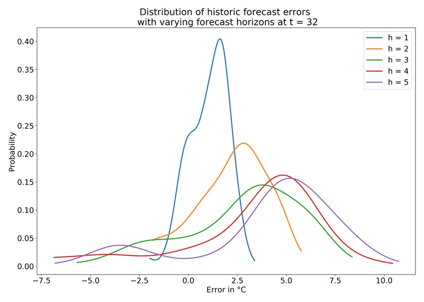
pattern is present. Figure 4 shows the empirical distributions of Moran’s I generated by
Monte Carlo repetitions under spatial randomisations. For this purpose, the temperatures
were randomised within their respective time periods and then Moran’s I was repeatedly
calculated (n = 1000). The graph of z-score standardised values contains not only the
empirical distributions in the null hypothesis, but also the z-score standardized eigenvalues of
the underlying matrices (i.e., either W or W ◦ U ). The latter eigenvalues give an indication
of the shape of the distribution of Moran’s I values [58]. What we see is that the distribution
using Equation 3 has a slight right skew, which is indicated by the clustering of eigenvalues
on the left margin of the distribution. This may complicate the determination of p-values
and the interpretation of Moran’s I. The method from Equation 2 behaves more similar to
the usual spatial weights matrix, which is an advantage of this method.
The results obtained for the case study of synthetic observations indicate that both of our
approaches proposed in this paper are not suitable for dealing with non-stationarity (Figure 5).
Recall the temporal periodicity present in the level of autocorrelation in this case study,
implying that observations are not necessarily related over time. Therefore, disregarding
Figure 4 Histogram and density estimates of the null distributions for the different Moran’s I
values calculated for the temperature case study. The black bars at the bottom of each plot indicate
the locations of the eigenvalues of each of the corresponding matrices used to calculate the respective
measures.D. Bucher, H. Martin, D. Jonietz, M. Raubal, and R. Westerholt 2:11
Figure 5 Different versions of Moran’s I calculated for two temporal periodic cycles of the
simulated data case study. All Moran’s I values are given in standardised form to facilitate the
readability of the figure. The bar at the top of the plot shows the simulated data.
certainty information of potential forecasts and simply using the baseline approach of only
taking into account samples taken during the same hour (resp. time interval) has led to the
best results for this case study, though also these are far from optimal (shown in blue in
Figure 5). This finding demonstrates the importance of complying with the assumptions of
Moran’s I. Otherwise, the non-stationarity may lead to the disclosure of spurious patterns,
which, in turn, may then lead to drawing wrong conclusions about geographic phenomena.
5 Conclusions
We put forward two ways of incorporating certainty information about sensor observations in
the estimation of Moran’s I. One of these approaches (Equation 2) uses an absolute notion of
incorporating raw certainty scores. The alternative approach (Equation 3) proposed is based
on the certainty of observations relative to others, that is, to the mean level of confidence
in forecasts. These approaches were applied to two case studies. One study uses real-world
temperatures and depicts one spatial process. The other one is based on synthetic values and
simulates a succession of temporally varying spatial processes, which is realised by alternating
the scale of the spatial patterns.
The results obtained show that using the best information available (relatively speaking)
and weighting them accordingly performs better than using only good information in an
absolute sense. The respective approach put forward in this paper (Equation 3) has, in com-
parison to ignoring time and reliability, led to a reduction of the systematic underestimation
of Moran’s I. The other approach presented here (Equation 2) is volatile and depends strongly
on a sufficient amount of trustworthy data being available. These results are informative
for the wider scholarly discussion on how to incorporate uncertainty in spatial measures
like Moran’s I. For future research, we recommend using certainty measures that work in a
relative manner by giving more weight to those observations which are above-average reliable.
In practice, researchers may use more sophisticated forecasting mechanisms, which may lead
to further improvements like pushing Moran’s I closer to the ground truth reference. Another
GIScience 20212:12 Moran’s I in the Context of Uncertain Mobile Sensor Measurements
important result of this study is that it was shown that non-stationarity is a source of uncer-
tainty that cannot be addressed by the approaches presented (or similar ones). This type of
uncertainty needs to be addressed differently and corresponding attempts should be targeted
in future research. Similarly, while the two presented case studies represent commonly found
phenomena, evaluating the methods on a wider range of sensor measurements and synthetic
data is required to further understand the impact of uncertainties arising due to different
spatial and temporal distributions and individual (inaccurate or faulty) sensors.
References
1 J Aldstadt, M Widener, and N Crago. Detecting irregular clusters in big spatial data. In
N. Xiao, M.-P. Kwan, M. F. Goodchild, and S. Shekhar, editors, Proceedings of the 7th
International Conference on Geographic Information Science (GIScience 2012), Columbus,
OH, 2012.
2 Lilia Angelova, Puck Flikweert, Panagiotis Karydakis, Daniël Kersbergen, Roos Teeuwen,
Kotryna Valečkaitė, Edward Verbree, Martijn Meijers, and Stefan van der Spek. Using a
dynamic sensor network to obtain spatiotemporal data in an urban environment. In Peter Kiefer,
Haosheng Huang, Nico Van de Weghe, and Martin Raubal, editors, Adjunct Proceedings of the
14th International Conference on Location Based Services, pages 13–18, Zürich, Switzerland,
2018. ETH Zurich.
3 Luc Anselin. Local indicators of spatial association—LISA. Geographical Analysis, 27(2):93–115,
1995.
4 Luc Anselin and Anil K Bera. Spatial dependence in linear regression models with an
introduction to spatial econometrics. In Aman Ullah and David E. A. Giles, editors, Handbook
of Applied Economic Statistics, pages 237–290. Marcel Dekker AG, New York, NY, 1998.
5 Renato M Assuncao and Edna A Reis. A new proposal to adjust Moran’s I for population
density. Statistics in Medicine, 18(16):2147–2162, 1999.
6 Matthias Bluemke, Bernd Resch, Clemens Lechner, René Westerholt, and Jan-Philipp Kolb.
Integrating geographic information into survey research: Current applications, challenges and
future avenues. Survey Research Methods, 11(3):307–327, 2017.
7 Jean-Pierre Bocquet-Appel and Robert R Sokal. Spatial autocorrelation analysis of trend
residuals in biological data. Systematic Zoology, 38(4):333–341, 1989.
8 Jean-Paul Chiles and Pierre Delfiner. Geostatistics: Modeling spatial uncertainty. John Wiley
& Sons, New York, NY, 2009.
9 Yongwan Chun and Daniel A Griffith. Spatial statistics and geostatistics: Theory and applica-
tions for geographic information science and technology. Sage, London, UK, 2013.
10 AD Cliff and JK Ord. The problem of spatial autocorrelation. London Papers in Regional
Science, pages 25–55, 1969.
11 AD Cliff and John K Ord. Space-time modelling with an application to regional forecasting.
Transactions of the Institute of British Geographers, pages 119–128, 1975.
12 Jens S Dangschat. Raumkonzept zwischen struktureller Produktion und individueller Kon-
struktion. Ethnologie und Raum, 9(1):24–44, 2007.
13 P De Jong, C Sprenger, and F Van Veen. On extreme values of Moran’s I and Geary’s c.
Geographical Analysis, 16(1):17–24, 1984.
14 Michel Denuit, Christian Genest, and Étienne Marceau. Stochastic bounds on sums of
dependent risks. Insurance: Mathematics and Economics, 25(1):85–104, 1999.
15 Mario Di Francesco, Sajal K Das, and Giuseppe Anastasi. Data collection in wireless sensor
networks with mobile elements: A survey. ACM Transactions on Sensor Networks, 8(1):7,
2011.
16 Jean Dubé and Diègo Legros. A spatio-temporal measure of spatial dependence: An example
using real estate data. Papers in Regional Science, 92(1):19–30, 2013.D. Bucher, H. Martin, D. Jonietz, M. Raubal, and R. Westerholt 2:13
17 Bradley Efron and Carl Morris. Stein’s estimation rule and its competitors – an empirical
Bayes approach. Journal of the American Statistical Association, 68(341):117–130, 1973.
18 Robert C Geary. The contiguity ratio and statistical mapping. The Incorporated Statistician,
5(3):115–146, 1954.
19 Arthur Getis. Reflections on spatial autocorrelation. Regional Science and Urban Economics,
37(4):491–496, 2007.
20 Arthur Getis. Spatial weights matrices. Geographical Analysis, 41(4):404–410, 2009.
21 Arthur Getis. Spatial autocorrelation. In Manfred M. Fischer and Arthur Getis, editors,
Handbook of Applied Spatial Analysis, pages 255–278. Springer, Heidelberg, Germany, 2010.
22 Arthur Getis. Analytically derived neighborhoods in a rapidly growing west african city: The
case of Accra, Ghana. Habitat International, 45:126–134, 2015.
23 Arthur Getis and J. K. Ord. The analysis of spatial association by use of distance statistics.
Geographical Analysis, 24(3):189–206, 1992.
24 Tilmann Gneiting. Probabilistic forecasting. Journal of the Royal Statistical Society. Series A
(Statistics in Society), pages 319–321, 2008.
25 Daniel A Griffith. A linear regression solution to the spatial autocorrelation problem. Journal
of Geographical Systems, 2(2):141–156, 2000.
26 Bruce Hajek. Random processes for engineers. Cambridge University Press, Cambridge, UK,
2015.
27 David Hasenfratz, Olga Saukh, Silvan Sturzenegger, and Lothar Thiele. Participatory air
pollution monitoring using smartphones. In Proceedings of the 2nd International Workshop
on Mobile Sensing: From Smartphones and Wearables to Big Data, Cambridge, MA, 2012.
Academic Press.
28 David Hasenfratz, Olga Saukh, Christoph Walser, Christoph Hueglin, Martin Fierz, Tabita
Arn, Jan Beutel, and Lothar Thiele. Deriving high-resolution urban air pollution maps using
mobile sensor nodes. Pervasive and Mobile Computing, 16:268–285, 2015.
29 Mary Hegarty, Daniel R Montello, Anthony E Richardson, Toru Ishikawa, and Kristin Lovelace.
Spatial abilities at different scales: Individual differences in aptitude-test performance and
spatial-layout learning. Intelligence, 34(2):151–176, 2006.
30 Bo Huang, Bo Wu, and Michael Barry. Geographically and temporally weighted regression
for modeling spatio-temporal variation in house prices. International Journal of Geographical
Information Science, 24(3):383–401, 2010.
31 Bret Hull, Vladimir Bychkovsky, Yang Zhang, Kevin Chen, Michel Goraczko, Allen Miu,
Eugene Shih, Hari Balakrishnan, and Samuel Madden. Cartel: a distributed mobile sensor
computing system. In Andrew Campbell, Philippe Bonnet, and John S. Heidemann, editors,
Proceedings of the 4th International Conference on Embedded Networked Sensor Systems, pages
125–138. ACM, 2006.
32 Paul H Jung, Jean-Claude Thill, and Michele Issel. Spatial autocorrelation statistics of
areal prevalence rates under high uncertainty in denominator data. Geographical Analysis,
51(3):354–380, 2019.
33 Teruyuki Kato, Yukihiro Terada, Masao Kinoshita, Hideshi Kakimoto, Hiroshi Isshiki, Ma-
sakatsu Matsuishi, Akira Yokoyama, and Takayuki Tanno. Real-time observation of tsunami
by RTK-GPS. Earth, Planets and Space, 52(10):841–845, 2000.
34 Roman Krzysztofowicz. The case for probabilistic forecasting in hydrology. Journal of
Hydrology, 249(1-4):2–9, 2001.
35 Jay Lee and Shengwen Li. Extending Moran’s index for measuring spatiotemporal clustering
of geographic events. Geographical Analysis, 49(1):36–57, 2017.
36 Yun Shin Lee and Stefan Scholtes. Empirical prediction intervals revisited. International
Journal of Forecasting, 30(2):217–234, 2014.
37 Fernando A López-Hernández and Coro Chasco-Yrigoyen. Time-trend in spatial dependence:
Specification strategy in the first-order spatial autoregressive model. Estudios de Economia
Aplicada, 25(2), 2007.
GIScience 20212:14 Moran’s I in the Context of Uncertain Mobile Sensor Measurements
38 Kevin M Lynch, Ira B Schwartz, Peng Yang, and Randy A Freeman. Decentralized environ-
mental modeling by mobile sensor networks. IEEE Transactions on Robotics, 24(3):710–724,
2008.
39 GD Makarov. Estimates for the distribution function of a sum of two random variables when
the marginal distributions are fixed. Theory of Probability & its Applications, 26(4):803–806,
1982.
40 Roger J Marshall. Mapping disease and mortality rates using empirical Bayes estimators.
Journal of the Royal Statistical Society: Series C (Applied Statistics), 40(2):283–294, 1991.
41 Russell L Martin and JE Oeppen. The identification of regional forecasting models using
space: Time correlation functions. Transactions of the Institute of British Geographers, pages
95–118, 1975.
42 Harvey J Miller. Tobler’s first law and spatial analysis. Annals of the Association of American
Geographers, 94(2):284–289, 2004.
43 Patrick AP Moran. Notes on continuous stochastic phenomena. Biometrika, 37(1/2):17–23,
1950.
44 Enrico Natalizio and Valeria Loscrí. Controlled mobility in mobile sensor networks: Advantages,
issues and challenges. Telecommunication Systems, 52(4):2411–2418, 2013.
45 Roger B. Nelsen. An introduction to copulas. Springer, New York, NY, 1999.
46 Neal Oden. Adjusting Moran’s I for population density. Statistics in Medicine, 14(1):17–26,
1995.
47 J Keith Ord and Arthur Getis. Local spatial autocorrelation statistics: Distributional issues
and an application. Geographical Analysis, 27(4):286–306, 1995.
48 J Keith Ord and Arthur Getis. Local spatial heteroscedasticity (LOSH). The Annals of
Regional Science, 48(2):529–539, 2012.
49 Edzer J Pebesma and Cees G Wesseling. Gstat: A program for geostatistical modelling,
prediction and simulation. Computers & Geosciences, 24(1):17–31, 1998.
50 Peter A Rogerson. The detection of clusters using a spatial version of the chi-square goodness-
of-fit statistic. Geographical Analysis, 31(2):130–147, 1999.
51 Ludger Rüschendorf. Random variables with maximum sums. Advances in Applied Probability,
pages 623–632, 1982.
52 Yasar Guneri Sahin. Animals as mobile biological sensors for forest fire detection. Sensors,
7(12):3084–3099, 2007.
53 Chenhua Shen, Chaoling Li, and Yali Si. Spatio-temporal autocorrelation measures for
nonstationary series: A new temporally detrended spatio-temporal Moran’s index. Physics
Letters A, 380(1-2):106–116, 2016.
54 Steven M Smith and Edward Vela. Environmental context-dependent memory: A review and
meta-analysis. Psychonomic Bulletin & Review, 8(2):203–220, 2001.
55 Enrico Steiger, René Westerholt, and Alexander Zipf. Research on social media feeds–A
GIScience perspective. In Christina Capineri, Muki Haklay, Haosheng Huang, Vyron Anto-
niou, Juhani Kettunen, Frank Ostermann, and Ross Purves, editors, European Handbook of
Crowdsourced Geographic Information, pages 237–254. Ubiquity Press, London, UK, 2016.
56 Xing Su, Hanghang Tong, and Ping Ji. Activity recognition with smartphone sensors. Tsinghua
Science and Technology, 19(3):235–249, 2014.
57 Mila Sugovic and Jessica K Witt. An older view on distance perception: Older adults perceive
walkable extents as farther. Experimental Brain Research, 226(3):383–391, 2013.
58 Michael Tiefelsdorf and Barry Boots. The exact distribution of Moran’s I. Environment and
Planning A, 27(6):985–999, 1995.
59 Michael Tiefelsdorf, Daniel A Griffith, and Barry Boots. A variance-stabilizing coding scheme
for spatial link matrices. Environment and Planning A, 31(1):165–180, 1999.
60 Waldo R Tobler. A computer movie simulating urban growth in the Detroit region. Economic
Geography, 46(sup1):234–240, 1970.D. Bucher, H. Martin, D. Jonietz, M. Raubal, and R. Westerholt 2:15
61 Sabrina Wahl, Christoph Bollmeyer, Susanne Crewell, Clarissa Figura, Petra Friederichs,
Andreas Hense, Jan D Keller, and Christian Ohlwein. A novel convective-scale regional
reanalysis COSMO-REA2: Improving the representation of precipitation. Meteorologische
Zeitschrift, 26(4):345–361, 2017.
62 Thomas Waldhör. The spatial autocorrelation coefficient Moran’s I under heteroscedasticity.
Statistics in Medicine, 15(7-9):887–892, 1996.
63 SD Walter. The analysis of regional patterns in health data: I. Distributional considerations.
American Journal of Epidemiology, 136(6):730–741, 1992.
64 SD Walter. The analysis of regional patterns in health data: II. The power to detect
environmental effects. American Journal of Epidemiology, 136(6):742–759, 1992.
65 Elisabeth M Weiss, Georg Kemmler, Eberhard A Deisenhammer, W Wolfgang Fleischhacker,
and Margarete Delazer. Sex differences in cognitive functions. Personality and Individual
Differences, 35(4):863–875, 2003.
66 Karl F Wender, Daniel Haun, Björn Rasch, and Matthias Blümke. Context effects in memory
for routes. In Christian Freksa, Wilfried Brauer, Christopher Habel, and Karl F. Wender,
editors, International Conference on Spatial Cognition (Spatial Cognition III), pages 209–231,
Heidelberg, Germany, 2002. Springer.
67 René Westerholt. The impact of the spatial superimposition of point based statistical config-
urations on assessing spatial autocorrelation. In A. Mansourian, P. Pilesjö, L. Harrie, and
R. von Lammeren, editors, Geospatial Technologies for All: Short Papers, Posters and Poster
Abstracts of the 21th AGILE Conference on Geographic Information Science, Lund, Sweden,
2018.
68 René Westerholt, Bernd Resch, Franz-Benjamin Mocnik, and Dirk Hoffmeister. A statistical
test on the local effects of spatially structured variance. International Journal of Geographical
Information Science, 32(3):571–600, 2018.
69 René Westerholt, Bernd Resch, and Alexander Zipf. A local scale-sensitive indicator of spatial
autocorrelation for assessing high-and low-value clusters in multiscale datasets. International
Journal of Geographical Information Science, 29(5):868–887, 2015.
70 René Westerholt, Enrico Steiger, Bernd Resch, and Alexander Zipf. Abundant topological
outliers in social media data and their effect on spatial analysis. PLOS ONE, 11(9):e0162360,
2016.
71 WH Williams and ML Goodman. A simple method for the construction of empirical confidence
limits for economic forecasts. Journal of the American Statistical Association, 66(336):752–754,
1971.
72 Min Xu, Chang-Lin Mei, and Na Yan. A note on the null distribution of the local spatial
heteroscedasticity (LOSH) statistic. The Annals of Regional Science, 52(3):697–710, 2014.
GIScience 2021You can also read