Space-time dependence of compound hot-dry events in the United States: assessment using a multi-site multi-variable weather generator - Earth ...
←
→
Page content transcription
If your browser does not render page correctly, please read the page content below
Earth Syst. Dynam., 12, 621–634, 2021
https://doi.org/10.5194/esd-12-621-2021
© Author(s) 2021. This work is distributed under
the Creative Commons Attribution 4.0 License.

                Space–time dependence of compound hot–dry
                events in the United States: assessment using
                 a multi-site multi-variable weather generator
                                Manuela I. Brunner, Eric Gilleland, and Andrew W. Wood
                       Research Applications Laboratory, National Center for Atmospheric Research,
                                       3450 Mitchell Ln, Boulder, CO 80301, USA
                   Correspondence: Manuela I. Brunner (manuela.brunner@hydrology.uni-freiburg.de)
                                             and Eric Gilleland (ericg@ucar.edu)
                                Received: 10 February 2021 – Discussion started: 11 February 2021
                            Revised: 13 April 2021 – Accepted: 22 April 2021 – Published: 19 May 2021

       Abstract. Compound hot and dry events can lead to severe impacts whose severity may depend on their
       timescale and spatial extent. Despite their potential importance, the climatological characteristics of these joint
       events have received little attention regardless of growing interest in climate change impacts on compound events.
       Here, we ask how event timescale relates to (1) spatial patterns of compound hot–dry events in the United States,
       (2) the spatial extent of compound hot–dry events, and (3) the importance of temperature and precipitation as
       drivers of compound events. To study such rare spatial and multivariate events, we introduce a multi-site multi-
       variable weather generator (PRSim.weather), which enables generation of a large number of spatial multivariate
       hot–dry events. We show that the stochastic model realistically simulates distributional and temporal autocorre-
       lation characteristics of temperature and precipitation at single sites, dependencies between the two variables,
       spatial correlation patterns, and spatial heat and meteorological drought indicators and their co-occurrence prob-
       abilities. The results of our compound event analysis demonstrate that (1) the northwestern and southeastern
       United States are most susceptible to compound hot–dry events independent of timescale, and susceptibility de-
       creases with increasing timescale; (2) the spatial extent and timescale of compound events are strongly related
       to sub-seasonal events (1–3 months) showing the largest spatial extents; and (3) the importance of temperature
       and precipitation as drivers of compound events varies with timescale, with temperature being most important
       at short and precipitation at seasonal timescales. We conclude that timescale is an important factor to be con-
       sidered in compound event assessments and suggest that climate change impact assessments should consider
       several timescales instead of a single timescale when looking at future changes in compound event characteris-
       tics. The largest future changes may be expected for short compound events because of their strong relation to
       temperature.

1   Introduction                                                   Fuchs et al., 2012). The US has been shown to be affected
                                                                   by concurrent hot and dry events at different timescales in-
Compound hot and dry events, i.e., events that are extreme         cluding short and long events effective at weekly to monthly
with respect to both temperature and precipitation, can lead       (Zhang et al., 2020) and seasonal to annual timescales (Al-
to severe impacts on agriculture and other sectors as il-          izadeh et al., 2020), respectively. The interest in these im-
lustrated by the 2010 heatwave–drought in Russia and the           pactful compound events is reflected in an increasing num-
2012 heatwave–drought in the central United States (US;            ber of studies assessing changes in their frequency of oc-
Mo and Lettenmaier, 2015), which led to substantial reduc-         currence. Substantial increases in the number of concurrent
tions in crop yields (Wegren, 2011; Christian et al., 2020;        droughts and heatwaves over the last few decades that are

Published by Copernicus Publications on behalf of the European Geosciences Union.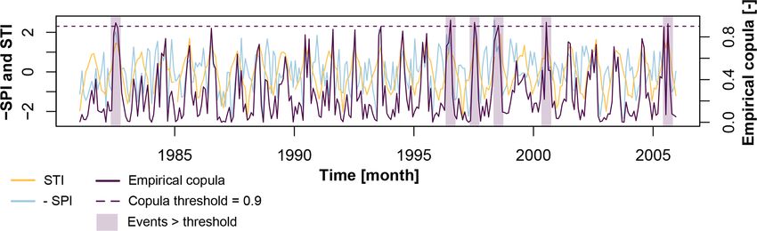
622                                                                                  M. I. Brunner et al.: Spatial hot–dry events

partly explained by increasing temperatures have been re-           and often applied to one variable, e.g., flood peaks. On the
ported not just for the US (Alizadeh et al., 2020; Mazdiyasni       other hand, continuous stochastic approaches, such as autore-
and AghaKouchak, 2015; Tavakol et al., 2020) but also glob-         gressive moving-average-type models (Stedinger and Taylor,
ally (Feng et al., 2020; Sarhadi et al., 2018) and for other re-    1982) or bootstrap approaches (Rajagopalan et al., 2010),
gions of the world such as China (Wu et al., 2019; Zhou and         do not represent spatial dependencies well. Therefore, Brun-
Liu, 2018; Yu and Zhai, 2020) and Europe (Manning et al.,           ner and Gilleland (2020) recently proposed a novel stochas-
2019).                                                              tic approach for simulating continuous streamflow time se-
   While frequency of occurrence is an important factor de-         ries in multiple catchments based on the wavelet trans-
termining impacts, the severity of impacts related to com-          form. The Phase Randomization Simulation using wavelets
pound events likely also depends on their spatial extent, i.e.,     (PRSim.wave) model combines an empirical spatiotemporal
how large the affected region is, and their timescale, i.e.,        model based on the wavelet transform and phase randomiza-
whether they just last weeks or extend over a longer period of      tion with the flexible four-parameter kappa distribution and
time. Indeed, spatiotemporal behavior is a common target of         builds on an earlier univariate version of the model (PRSim;
analyses in general for drought, a related phenomenon, as in        Brunner et al., 2019). It is able to simulate continuous, spa-
the multi-temporal severity-area-duration analyses presented        tially consistent time series but has so far only been applied
by Andreadis et al. (2005). Despite their potential importance      to one variable (streamflow).
for understanding and projecting the physical manifestation            We extend PRSim.wave here to multiple variables by
and impacts of compound events, these spatiotemporal char-          proposing a multi-site multi-variable stochastic weather gen-
acteristics have received comparably little attention. Only re-     erator (PRSim.weather) that simulates long time series of
cently have Alizadeh et al. (2020) and Wu et al. (2021) shown       spatially consistent temperature (T ) and precipitation (P )
that the area affected by concurrent hot–dry extremes has           time series. This multi-site multi-variable stochastic model
increased significantly over the past few decades in the US         reproduces local variable distributions using flexible dis-
and globally for long, i.e., seasonal, timescales. However, it      tributions for T and P and introduces spatiotemporal and
remains to be investigated how the timescale of compound            variable dependence using the wavelet transform (Torrence
events influences their characteristics and spatial extent.         and Compo, 1998) and phase randomization (Schreiber and
   This study aims to deepen our understanding of how the           Schmitz, 2000; Lancaster et al., 2018). Using this multi-site
timescale of compound hot–dry events in the US relates to           multi-variable generator to simulate a large set of spatial mul-
(1) spatial patterns of compound event affectedness (i.e.,          tivariate hot–dry events will help to shed light on the ques-
where in the US hot–dry events are most frequent), (2) spatial      tion of how timescale shapes compound event characteristics
extents of compound events (i.e., how large compound events         including spatial extent. Thus, this analysis will provide cru-
are), and (3) the role of temperature and precipitation as          cial information to increase preparedness and develop adap-
drivers of compound events by focusing on multivariate and          tation measures for potentially impactful spatial multivariate
spatial extreme events (Zscheischler et al., 2020). To answer       events.
the question of how timescale shapes compound event char-
acteristics, we determine the probability, extent, and drivers      2     Methods and materials
of spatial multivariate heatwaves and meteorological drought
over the conterminous US (CONUS) for different timescales           We develop a multi-variable multi-site weather generator that
ranging from weekly to annual events.                               stochastically simulates spatially consistent daily T and P
   Studying such spatial multivariate events is challenging         time series for a large number of locations. We apply this
because they are rare in observational records (Zscheischler        model to a gridded T and P data set in the CONUS to gener-
et al., 2018). This challenge can, for example, be tackled          ate a large sample of spatial multivariate hot–dry events. We
by developing stochastic simulation approaches to generate          subsequently use this sample to determine which regions in
large data sets with similar statistical properties as the obser-   the US are susceptible to compound events and large spatial
vations (Vogel and Stedinger, 1988). A stochastic approach          multivariate event extents at different timescales. Last, we
to simulate spatial multivariate hot–dry events at different        look at how the importance of T and P for compound event
timescales needs to (1) represent spatial dependencies be-          development varies with timescale.
tween sites to capture the spatial aspect, (2) represent de-
pendencies between variables to capture dependencies be-
                                                                    2.1    Study region and data
tween precipitation and temperature, and (3) be continuous
to enable studying timescales from weeks to years. How-             The analysis is performed using a gridded data set of daily T
ever, existing models often only fulfill one or two of these        and P time series for 894 equally spaced grid cells in the
three requirements. On the one hand, existing spatial mod-          CONUS. T and P data were obtained from the ERA5-
els for simulating spatial extreme events, such as the con-         Land reanalysis for the period 1981–2018 (ECMWF, 2019).
ditional exceedance model by Heffernan and Tawn (2004),             ERA5-Land relies on atmospheric forcing from the ERA5
are event-based (Keef et al., 2013; Diederen et al., 2019)          reanalysis (Hersbach et al., 2020) and provides variables at

Earth Syst. Dynam., 12, 621–634, 2021                                                  https://doi.org/10.5194/esd-12-621-2021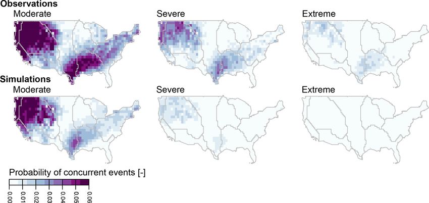
M. I. Brunner et al.: Spatial hot–dry events                                                                                                 623

a spatial resolution of 9 km for the period of 1981 to the                             a gamma-like distribution and a heavy-tailed general-
present. We chose a subset of regularly spaced grid cells                              ized Pareto distribution (GPD) thanks to a transforma-
by sampling 1500 grid cells over the extent of the CONUS,                              tion function G(v) (Naveau et al., 2016). The E-GPD is
which resulted in 894 grid cells over land that are used for                           defined as
this analysis.                                                                         F {x} = G[Hθ {x/σ }],
                                                                                                       (
                                                                                                         1 − (1 + θ z)−1/θ     if θ 6 = 0,
2.2     Methods                                                                        where Hθ (z) =                                        (2)
                                                                                                         1 − e−z               if θ = 0,
2.2.1    Stochastic multi-site multi-variable modeling
                                                                                       where σ > 0 is a scale parameter, θ is the shape param-
To study compound hot–dry events, we develop a multi-site                              eter of the GPD, and G(v) = v ρ . The E-GPD has been
multi-variable weather generator, PRSim.weather, that en-                              demonstrated to be valuable in multi-site precipitation
ables simulation of large sets of spatially consistent com-                            modeling thanks to its flexibility (Evin et al., 2018).
pound hot–dry events at a daily scale. PRSim.weather                                   The parameters of the E-GPD distribution are estimated
combines an empirical spatiotemporal model based on the                                using probability weighted moments (R package mev;
wavelet transform and phase randomization with two flexi-                              Belzile et al., 2020). We use the E-GPD to simulate
ble parametric distributions for T and P , which enables ex-                           nonzero precipitation values and complement it with as
trapolation to yet unobserved values. It builds on the spatial                         many zero values as in the observations to obtain the
stochastic model PRSim.wave (Phase Randomization Sim-                                  full P distribution with an appropriate probability of
ulation using wavelets) proposed by Brunner and Gilleland                              precipitation occurrence.
(2020), which simulates continuous streamflow time series at
                                                                                    3. Transform the T and P time series from the time
multiple sites. We expand the functionality of PRSim.wave
                                                                                       to the frequency domain by decomposing the series
to simulate multiple variables, i.e., T and P , at multiple
                                                                                       into an amplitude and phase signal using a continuous
sites. The weather generation procedure implemented in
                                                                                       wavelet transform with the Morlet wavelet (Torrence
PRSim.weather consists of five main steps (Fig. 1).
                                                                                       and Compo, 1998) (R package wavScalogram; Bolós
 1. Feed in observed daily T and P time series for multiple                            and Benítez, 2020). The continuous wavelet transform
    sites (here grid cells).                                                           is defined as the convolution of a time series xn of
                                                                                       length n:
 2. Fit monthly distributions to T and P time series at each                                    N−1          0
                                                                                                          ∗ (n − n)δt
                                                                                                 X
    site to capture seasonal variations in distribution pa-                            Wn (l) =       xn ψ0
                                                                                                        0               ,                (3)
    rameters (i.e., one separate distribution is fitted to the                                  n0 =0
                                                                                                                l
    data in each month). Using theoretical instead of em-
                                                                                       where the (*) indicates the complex conjugate, l the
    pirical distributions will allow us to generate extreme
                                                                                       wavelet scale, and ψ0 (η) the Morlet wavelet, which is
    values more extreme than the observations. For T , we
                                                                                       defined as
    use the flexible skewed exponential power (SEP) dis-                                                            2 /2
    tribution with four parameters (Fernández and Steel,                               ψ0 (η) = π −1/4 eiω0 η e−η          ,                 (4)
    1998), which generalizes the Gaussian distribution, can
                                                                                       where η is a nondimensional time parameter,
                                                                                                                         √         ω0 is the
    reproduce different skewness and kurtosis, and has been
                                                                                       nondimensional frequency, and i = −1 is the imagi-
    previously applied for multi-site temperature simulation
                                                                                       nary unit.
    (Evin et al., 2019). The SEP distribution is defined as
                                                                                    4. Generate one random time series using bootstrap re-
                    [κ 2 /(1 + κ 2 )]γ {[(ξ − x)/(ακ)]h , 1/ h} for x < ξ

      F (x) =                                                             ,   (1)      sampling on the temperature time series of one ran-
                    1 − [1/(1 + κ 2 )]γ {[κ(x − ξ )/α]h , 1/ h} for x ≥ ξ              domly sampled site by sampling years with replace-
                                                                                       ment. Use the wavelet transform to also decompose this
      with location parameter ξ , scale parameter α, shape pa-
                                                                                       bootstrapped series in order to obtain a random phase
      rameters κ and h, and γ (Z, α) representing the upper
                                                                                       signal.
      tail of the incomplete gamma function (Asquith, 2014).
      The parameters of the SEP distribution are estimated                          5. Generate stochastic time series for T and P by ap-
      using L-moments (R package lmomco; Asquith, 2020).                               plying the inverse wavelet transform to the observed
      For P , we use an extended generalized Pareto distribu-                          amplitude signals and the randomly generated phases.
      tion (E-GPD; Papastathopoulos and Tawn, 2013) with                               Rank-transform the newly generated time series using
      three parameters to model positive precipitation val-                            the probability integral transform to the desired distri-
      ues. The E-GPD jointly models non-extreme and ex-                                bution for each month using the monthly distribution
      treme values of P while bypassing the threshold selec-                           parameters derived in Step 2 (SEP parameters for T and
      tion problem as it enables smooth transitioning between                          E-GPD parameters for P ).

https://doi.org/10.5194/esd-12-621-2021                                                               Earth Syst. Dynam., 12, 621–634, 2021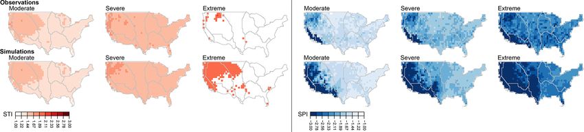
624                                                                                              M. I. Brunner et al.: Spatial hot–dry events

Figure 1. Illustration of the five working steps of PRSim.weather: (1) feed in daily observed temperature (T ) and precipitation (P ) time series
for multiple sites (1, . . ., n); (2) fit SEP distribution to T and E-GP distribution to P time series of all sites at a monthly scale; (3) decompose T
and P time series of all sites into an amplitude (A) and phase (P) signal using the wavelet transform; (4) generate one random time series
using bootstrap resampling and decompose that random series into an amplitude and phase signal too; and (5) generate random daily T
and P time series by combining the observed amplitude signal of each site and variable with the randomly generated phase signal and by
back-transforming the signals to the time domain using the inverse wavelet transform. Rank-transform the newly generated signal to the
desired distribution using the parameter estimates from Step 2.

   The simulation of yet unobserved magnitudes becomes                        convert the T and P series to weekly and monthly series us-
possible thanks to the use of parametric distributions for T                  ing mean values and sums, respectively. We work with aggre-
and P in Step 2. The spatial and variable dependencies are                    gation levels of 1 week to represent “flash” compound events
introduced in Step 5 by using the same random phases in the                   and of 1, 3, 6, and 12 months to represent sub-seasonal, sea-
wavelet transform at all sites and for both variables.                        sonal, and annual timescales. In a second step, we transform
   The stochastic multi-site multi-variable model is evaluated                the aggregated T and P series to series of standardized in-
with respect to the following characteristics: (1) T and P dis-               dices, which we will use to study relationships between the
tributions (CDFs) at individual sites, (2) temporal autocorre-                marginal behavior of compound events because they guaran-
lation of T and P (ACFs) at individual sites, (3) spatial de-                 tee variable and site comparability. Standardized precipita-
pendencies across sites for T and P (variograms), (4) T –P                    tion index (SPI) series (McKee et al., 1993) for each loca-
variable dependencies (scatter plots), and (5) simulated spa-                 tion are computed by transforming the P values to a stan-
tial patterns of the standardized temperature index (STI), the                dardized normal distribution (mean 0 and SD 1) using a
standardized precipitation index (SPI), and the probability of                site-specific E-GPD distribution (the Kolmogorov–Smirnov
compound high STI and low SPI anomalies at a 1-month ag-                      test did not reject gamma in over 80 % of the grid cells).
gregation level for moderate, severe, and extreme events ac-                  Similarly, we compute standardized temperature index series
cording to the empirical copula (see Sect. 2.2.2).                            (STI; Zscheischler et al., 2014) using the SEP distribution for
   PRSim.weather is finally run n = 100 times for the                         transformation. Last, compound hot–dry events are identified
894 grid cells in the US in order to substantially in-                        for each timescale and grid cell using a bivariate empirical
crease the sample size available for the assessment of com-                   copula (Deheuvels, 1979; Genest and Favre, 2007), which
pound hot–dry events by pooling the different model runs                      describes the joint distribution of T (STI) and P (SPI) with
(28 years · 100 = 2800 years).                                                uniform margins. We change the sign of the SPI values to
                                                                              convert negative to positive anomalies as we are interested in
                                                                              events during which STI and SPI are extreme. The empirical
2.2.2    Compound event analysis                                              copula of STI and SPI is described as
                                                                                               n
While the focus is on the simulated series, compound events                                 1X     Ri         Si
and their corresponding T and P characteristics are identi-                   Cn (u, v) =        1      ≤ u,     ≤v ,                              (5)
                                                                                            n i=1 n + 1      n+1
fied at different timescales in both the observed and stochas-
tically simulated time series to assess the reliability of the                where Ri and Si represent pairs of ranks (across STI and SPI
stochastic model. To look at different timescales, we first                   time series), n the sample size, and Cn (u, v) the rank-based

Earth Syst. Dynam., 12, 621–634, 2021                                                               https://doi.org/10.5194/esd-12-621-2021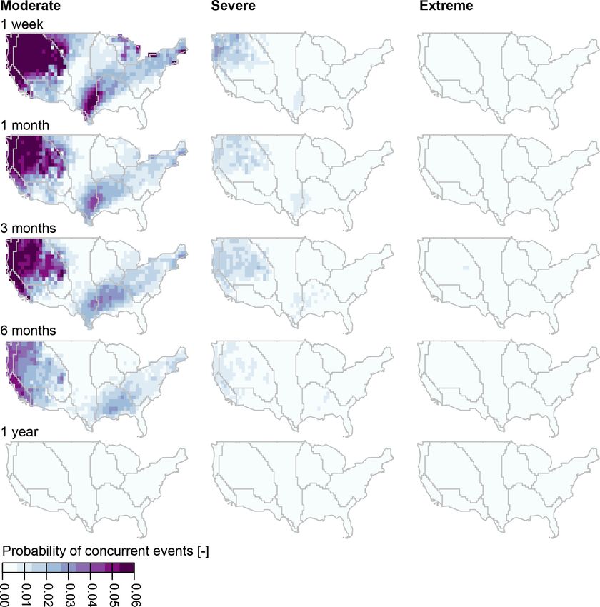
M. I. Brunner et al.: Spatial hot–dry events                                                                                              625

Figure 2. Illustration of the relationship between monthly STI (yellow) and SPI (blue) time series and their bivariate copula (i.e., the values
         Ri    Si
of Cn ( n+1 , n+1 ); purple) for one example grid cell. Compound STI and SPI events exceeding a copula-threshold of 0.9 are highlighted by
purple boxes.

estimator of the copula C(u, v). An example of how the em-                sess to which degree these two factors influence STI and SPI
pirical copula (purple) is related to the margins STI (yellow)            importance.
and SPI (blue) is provided in Fig. 2.
   Using the time series of empirical bivariate distribution
values, we identify moderate, severe, and extreme compound                3     Results
events using three thresholds at 0.8, 0.9, and 0.95, respec-
tively (see Fig. 2 for an example with a threshold of 0.9). This          3.1    Evaluating the weather generator
copula-based threshold procedure slightly differs from an ap-
                                                                          The multi-site multi-variable stochastic simulation approach
proach whereby both margins (SPI and STI) have to jointly
                                                                          in PRSim.weather is capable of reproducing the observed
exceed a threshold in order for an event to be defined as a
                                                                          statistical characteristics of T and P time series at individ-
compound event. The bivariate threshold procedure includes
                                                                          ual locations as illustrated by one example station (Fig. 3).
a slightly different event space, which besides the jointly
                                                                          The flexible SEP and E-GPD distributions capture the local T
marginally extreme events also includes those events that are
                                                                          and P distributions well as indicated by the good match of
extreme in terms of the bivariate distribution but not neces-
                                                                          simulated with observed densities (Fig. 3a and b). The suit-
sarily in terms of both margins. Please note that the focus on
                                                                          ability of the SEP and E-GPD distributions to model local T
high T and low P events leads to the selection of compound
                                                                          and P distributions also extends to the tails as 100-year re-
events in the summer season. For an aggregation period of
                                                                          turn levels estimated from the observed and simulated series
1 month, all selected compound events happen between May
                                                                          compare well for both variables. The temporal autocorrela-
and October, with over 90 % of the events happening in July
                                                                          tion in both variables is realistically reproduced, as shown by
or August. The seasonal focus is slightly shifted towards late
                                                                          the good agreement of simulated with observed autocorre-
summer (August) and early fall (September and October) as
                                                                          lation functions, thanks to the observed frequency spectrum
we move towards longer aggregation periods.
                                                                          information used in the inverse wavelet transform (Fig. 3c
   To assess the spatial extent of compound events at differ-
                                                                          and d). The simulated time series mimic the main tempo-
ent timescales, we define the spatial extent of the compound
                                                                          ral characteristics of the observed time series well, includ-
event as the percentage of grid cells affected by the com-
                                                                          ing seasonality and temporal event distribution and cluster-
pound event at any given timescale. Then, for each grid cell,
                                                                          ing as illustrated by 3 years of observed and simulated T
we determine the median spatial extent of those events it is
                                                                          and P data (Fig. 3e and f). The T –P variable dependence
affected by at each timescale.
                                                                          is also generally well captured thanks to the use of the same
   To explain the role of the individual variables T and P
                                                                          random phases for both variables when applying the inverse
in compound event occurrence, we compute Kendall’s cor-
                                                                          wavelet transform (Fig. 3g and h). However, the number of
relation between the median bivariate distribution (empiri-
                                                                          high T –low P events at a daily scale is slightly underesti-
cal copula) and the median standardized indices STI and SPI
                                                                          mated. The above-described model evaluation can be gener-
over all simulation runs at different timescales. This corre-
                                                                          alized to other grid cells in the data set. In addition to these
lation analysis is performed for nine hydroclimatic regions
                                                                          local characteristics, spatial correlations are captured as illus-
in the United States (Bukovsky; Bukovsky, 2011) to quan-
                                                                          trated by the similarity of observed and simulated variograms
tify the regional spread in the role of STI and SPI for com-
                                                                          (Fig. 4). However, the spatial correlation of T is slightly over-
pound event development; i.e., correlation is computed be-
                                                                          estimated by the simulations. Achieving a “perfect” joint rep-
tween median bivariate distributions and median STI or SPI
                                                                          resentation of the three forms of dependence – temporal, spa-
at different grid cells within a region. We look at correlations
                                                                          tial, and variable – is very challenging. The model is consid-
for different timescales and event extremeness levels to as-
                                                                          ered suitable for the analysis of compound hot–dry events

https://doi.org/10.5194/esd-12-621-2021                                                        Earth Syst. Dynam., 12, 621–634, 2021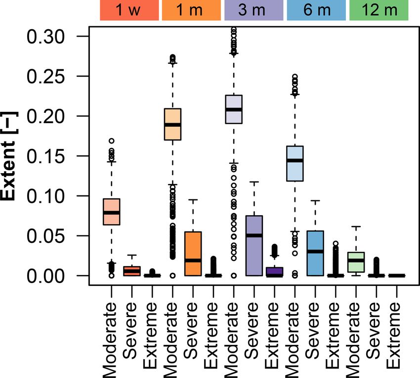
626                                                                                            M. I. Brunner et al.: Spatial hot–dry events

Figure 3. PRSim.weather evaluation for one example grid cell: (a, b) marginal distributions for observed and simulated T (orange) and P
(blue) (one line represents one simulation run), (c, d) temporal autocorrelation for observed and simulated T and P (one line represents one
simulation run), (e, f) 3-year time series of T (right y axis) and P (left y axis) for observations and simulations, and (g, h) heat scatter plot of
the P –T relationship in observations and simulations.

                                                                            comparing observed and simulated STI and SPI patterns for
                                                                            different levels of extremeness (Fig. 5). While the simulated
                                                                            spatial STI and SPI patterns look similar to the observed
                                                                            ones, they are more expressed because of the larger sam-
                                                                            ple available, which contains yet unobserved extremes be-
                                                                            cause of the use of parametric distributions for simulating T
                                                                            and P . The spatial pattern for STI is rather weak, with STI
                                                                            values being relatively homogeneously distributed except for
                                                                            the Pacific Northwest and along the west coast where STI
                                                                            values are slightly higher than in the rest of the country. In
Figure 4. PRSim.weather evaluation for spatial dependence: (a) ob-          contrast, the spatial pattern of median SPIs is expressed with
served vs. simulated T (orange) variograms for 92 equally spaced            substantially higher negative anomalies in the western than
grid cells and (b) observed vs. simulated P (blue) variograms for
                                                                            the eastern US and particularly strong negative anomalies in
92 grid cells, which describe the degree of spatial dependence of a
                                                                            the southwest.
field (Cressie, 1993).
                                                                               The spatial STI and SPI patterns are reflected in the spatial
                                                                            distribution of the probability of compound hot–dry events,
                                                                            which is also realistically represented but slightly underes-
because it has an acceptable performance with respect to all                timated by PRSim.weather (Fig. 6). The highest probability
three aspects and enables increasing the sample size of com-                of compound hot–dry events at a monthly timescale is found
pound events.                                                               in the Pacific Northwest, along the west coast, in the Rocky
   PRSim.weather enables simulation of a large sample of                    Mountains, and in the southeast, in particular in Texas. In
extreme events in terms of standardized temperature (STI)                   contrast, compound hot–dry events are relatively rare in the
and precipitation indices (SPI). These spatial samples enable               Great Plains, the midwest, and Florida. For the remainder of

Earth Syst. Dynam., 12, 621–634, 2021                                                             https://doi.org/10.5194/esd-12-621-2021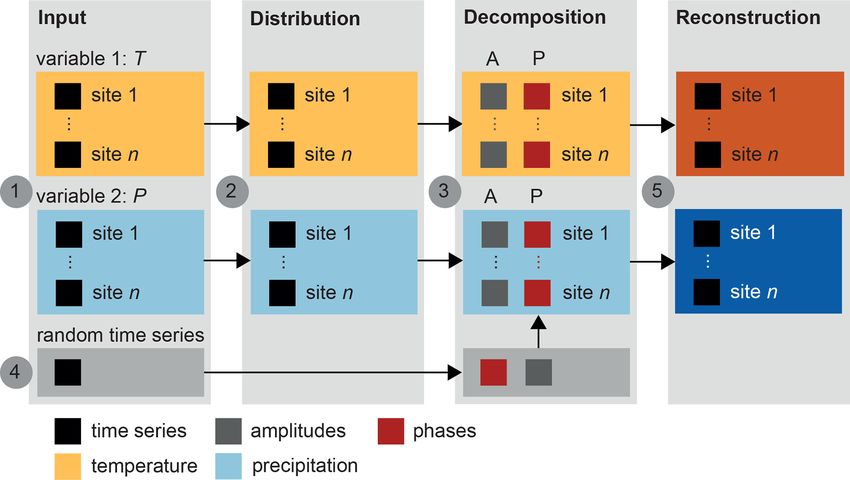
M. I. Brunner et al.: Spatial hot–dry events 627
Figure 5. Spatial distribution of median observed (upper panel) and simulated (lower panel) STIs (left panel) and SPIs (right panel) at
a monthly timescale for three levels of extremeness: moderate (STI > 1 and SPI < −1), severe (STI > 1.5 and SPI < −1.5), and extreme
(STI > 2 and SPI < −2). The darker the color, the more severe the median events in a certain grid cell.
Figure 6. Spatial distribution of observed (upper panel) and simulated (lower panel) probability of occurrence of hot–dry events (number
of compound events compared to the total number of months) at a monthly timescale for three levels of extremeness: moderate (Cn > 0.8),
severe (Cn > 0.9), and extreme (Cn : 0.95). The darker the color, the more likely compound hot–dry events are.
our analysis, we focus on the stochastic simulations because with increasing timescale and event extremeness. At an an-
of their large sample size, which allows us to study rare spa- nual timescale, the probability of events at all extreme thresh-
tial multivariate hot–dry events. olds is negligible.
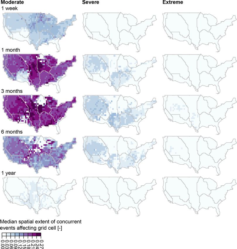
Different regions of the US differ not only in how suscep-
tible they are to compound hot–dry event occurrence but also
3.2 Compound hot–dry events in how likely they are to be affected by a widespread (large
spatial scale) compound event. The spatial occurrence pat-
The stochastically simulated compound hot–dry events re-
terns for spatially extensive compound hot–dry events vary
veal that the probability of co-occurring hot and dry peri-
by timescale (Fig. 8). For moderate extremes, the midwest is
ods is highest in the northwestern and southeastern US in-
the most affected by large events, with more prevalence in the
dependently of the timescale considered (Fig. 7). However,
upper midwest at shorter timescales and the central to south-
the probability of compound events decreases with increas-
ern midwest at longer timescales. For the severe category, the
ing duration, as can be expected due to the aggregation over
western and southeastern regions are more affected, which is
increasingly longer periods of multiple weather events that
a similar spatial pattern as the probability of compound hot–
may not all favor instantaneous compound hot–dry condi-
dry events (Fig. 7), although there are no large-scale events
tions and joint extremeness. Still, there are spatial nuances
at a short timescale. In addition, large compound events gen-
depending on the timescale considered. For example, the
erally become less likely as we move beyond the 3-month
high probabilities of compound events are located in the
timescale and toward extreme events (Fig. 9). While ∼ 20 %
south for short timescales and move to the southeast as we
of the CONUS may be jointly affected by moderate and short
move towards longer timescales. Timescale not only affects
compound events, spatial extents of compound events be-
local concurrence probabilities but also the size of the re-
gions affected by compound hot–dry events, which decreases
https://doi.org/10.5194/esd-12-621-2021 Earth Syst. Dynam., 12, 621–634, 2021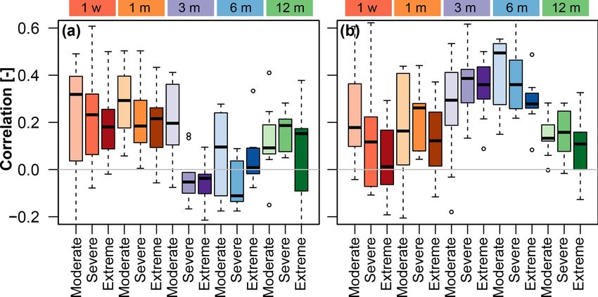
628                                                                                       M. I. Brunner et al.: Spatial hot–dry events

Figure 7. Probability of compound hot–dry events (number of compound events compared to the total number of months) at different
timescales (1 week, 1 month, 3 months, 6 months, 1 year) and for three levels of extremeness (moderate Cn > 0.8, severe Cn > 0.9, and
extreme Cn > 0.95) per grid cell. The darker the color, the higher the probability that a grid cell is affected by compound hot–dry events.

come small to nonexistent for extreme and long-lasting (i.e.,           reproduces the distributional and temporal autocorrelation
annual) compound events.                                                characteristics of T and P at single sites, the dependence
   The importance of T (STI) and P (SPI) as drivers of                  between the two variables, the spatial correlation of T and P
compound events varies by timescale and level of extreme-               across sites, and spatial patterns of STI, SPI, and their
ness (Fig. 10). T is a particularly important driver at short           concurrence probabilities. However, spatial dependencies
timescales, as indicated by the high correlation between me-            are slightly overestimated, while variable dependencies
dian STI and the median bivariate distribution of grid cells            are slightly underestimated. The model still has acceptable
within a specific hydroclimatic region (Fig. 10a). The impor-           performance across three types of dependencies – temporal,
tance of P as a driver of compound events increases with                spatial, and variable – and enables studying rare spatial
timescale up to event durations of 6 months but decreases               multivariate events, which would not be possible using
with level of extremeness (Fig. 10b). In summary, the longer            observations only. Please note that even though the model
the timescale, the more important P becomes as a driver                 generates yet unobserved observations, the simulations
compared to T (up to a seasonal timescale).                             are not independent of the limited sample size used to fit
                                                                        the model because the model is data-driven like any other
                                                                        calibrated and/or fitted model. Please also note that while
4   Discussion                                                          the model will be able to retain the statistical dependencies
                                                                        between variables to some degree, individual simulated
The    multi-site    multi-variable   stochastic   model                events may not necessarily be physically consistent if many
PRSim.weather proposed for the joint simulation of T                    variables are jointly simulated. We note that stochastic
and P at multiple sites has been shown to be suitable for               approaches may be combined with physical approaches,
the simulation of spatial multivariate hot–dry events. It

Earth Syst. Dynam., 12, 621–634, 2021                                                       https://doi.org/10.5194/esd-12-621-2021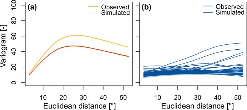
M. I. Brunner et al.: Spatial hot–dry events                                                                                           629

Figure 8. Spatial patterns of median compound event extent per grid cell for different timescales and extremeness levels over nine hydrocli-
matic regions. The darker the color, the higher the median spatial extent of compound events a grid cell is affected by.

such as in the weather generator AWE-GEN-2 by Peleg                     ity. Extending model application to nonstationary conditions
et al. (2017), or one may rely on large climate ensemble                would require the implementation of nonstationary distribu-
simulation approaches (Deser et al., 2020; Bevacqua et al.,             tions for both T and P . For example, one could introduce co-
2021).                                                                  variates for certain parameters of the marginal distributions
   Further model development should focus on how to im-                 of T and P in Step 2 or introduce covariates with information
prove the representation of dependencies in very high T –               about trends or variability in P and/or T to guide resampling
low P events at a daily scale and applications in other con-            in Step 4.
texts as well as under nonstationary conditions. While the                 The finding that the western and southeastern US are most
current application focuses on the two variables T and P in             likely to be affected by compound hot–dry events at sub-
the US, the model can be adapted to other regions, other vari-          annual timescales suggests that the likelihood of compound
ables, and a multivariate context in which more than two vari-          events is somehow related to precipitation seasonality, with
ables are of interest. Adapting the model to other regions and          regions receiving most of their precipitation in winter or
variables requires reconsidering distribution choices, and ex-          spring and comparably less in summer and fall (Finkelstein
tending it to a multivariate context necessitates adding more           and Truppi, 1991) being the most likely to be affected by
input variables, which are subsequently randomized in the               compound events. In “normal” years, both the western and
same way as all other variables. Potential multivariate ap-             southeastern US receive a large part of their precipitation
plications include the simulation of spatial concurrent plu-            through recurrent patterns such as atmospheric rivers (Rutz
vial, river, and coastal flooding by jointly modeling precipi-          et al., 2015) and tropical cyclones (Kunkel et al., 2012), re-
tation, discharge, and water levels or the joint simulation of          spectively. Anomalies can arise because of temporal shifts
wildfire drivers such as wind speed, temperature, and humid-            or a weakening of these patterns in specific seasons and/or

https://doi.org/10.5194/esd-12-621-2021                                                      Earth Syst. Dynam., 12, 621–634, 2021
630                                                                                    M. I. Brunner et al.: Spatial hot–dry events

                                                                      The importance of temperature as a driver of short and ex-
                                                                      treme compound hot–dry events suggests that the increasing
                                                                      temperatures associated with climate change may induce fu-
                                                                      ture changes in the frequency and magnitude of short and
                                                                      extreme compound events. Such future increases have been
                                                                      projected globally (Wu et al., 2021) and regionally, e.g., for
                                                                      China (Zhou and Liu, 2018). In addition, previous studies
                                                                      have shown that the number and intensity of compound hot–
                                                                      dry events may increase because temperature and precipi-
                                                                      tation may become increasingly coupled and/or correlated
                                                                      in summer (De Luca et al., 2020; Zscheischler and Senevi-
                                                                      ratne, 2017), possibly as a consequence of an intensification
                                                                      of land–atmosphere feedbacks (Seneviratne et al., 2010). As
                                                                      the number of compound events increases locally, the area
                                                                      exposed to compound hot–dry events is projected to increase
                                                                      with global warming (Vogel et al., 2019), continuing a trend
Figure 9. Relationship between compound event extent, timescale,      that has been already observed during the past few decades
and event extremeness. Box plots summarize the spread of me-          (Alizadeh et al., 2020). How exactly future changes in com-
dian extent (percentage of overall area affected) across grid cells   pound event extents relate to changes in drought spatial ex-
for weekly (red), monthly (orange), 3-monthly (purple), 6-monthly     tent (Brunner et al., 2021) and in heatwave spatial extent re-
(blue), and annual (green) timescales and three levels of extreme-
                                                                      mains to be investigated.
ness: moderate, severe, and extreme.

                                                                      5   Summary and conclusions
years. In addition, the regions most likely to experience com-
pound events are the regions found to be most susceptible to          We introduce the multi-variable multi-site stochastic model
heatwaves in the US (Smith et al., 2013).                             PRSim.weather to simulate continuous and spatially con-
   Our finding that the spatial extents of compound events            sistent multivariate time series. The model is shown to re-
are largest for moderate events at sub-seasonal timescales            alistically simulate distributional and temporal autocorrela-
implies that while these moderate events may have less se-            tion characteristics of temperature and precipitation at single
vere impacts at a local scale, they may still be highly relevant      sites, dependencies between the two variables up to moder-
at a regional scale. Compound events with large spatial ex-           ate extremes, spatial correlation patterns, and spatial heat and
tents represent a particular management challenge because             drought indicators as well as their co-occurrence probabili-
they may preclude the transfer of resources and emergency             ties for a gridded large-sample data set in the United States.
supplies from one to another region. Consequently, the so-            However, future work is needed to improve the representa-
cietal impacts of large-scale compound events can be ampli-           tion of very extreme hot–dry events. We apply the stochas-
fied, since many coping strategies are predicated on some de-         tic model to generate a large set of spatial and multivariate
gree of resource transfer from less severely affected adjacent        hot–dry events and use these simulated compound events to
regions (Murgatroyd and Hall, 2020).                                  assess how event timescale and extremeness influence the
   The finding that temperature is a comparably more impor-           spatial affectedness by compound hot–dry events over the
tant driver for short compound events only, while precipi-            United States, the spatial extent of compound events, and
tation is comparably more important at seasonal timescales,           their main drivers temperature and precipitation. Our results
corroborates the findings of previous studies about the im-           show that (1) the northwest and southeast are most likely
portance of different hydrometeorological drivers at differ-          to be affected by compound hot–dry events independent of
ent timescales. Zhang et al. (2020) have shown that temper-           timescale; (2) the spatial extent of compound hot–dry events
ature is the most important hydrometeorological driver of             decreases with increasing event extremeness and timescale,
short-term compound hot–dry extremes, which aligns with               i.e., the events with the largest spatial extents are typically
our findings. In addition, Tavakol et al. (2020) have shown           short and only moderately extreme; and (3) temperature is
that at long (i.e., annual) timescales, hot–dry–windy events          an important driver of short compound events, while pre-
co-occurred with major heatwaves, which is in line with our           cipitation is an important driver at seasonal timescales, par-
finding that temperature is an important driver of extreme            ticularly for the moderately extreme events. These findings
compound hot–dry events at seasonal to annual timescales.             highlight the fact that occurrences of compound events are
   Future changes in the frequency and severity of compound           strongly influenced by the timescales at which they are de-
hot–dry events are expected because of changes in both tem-           fined. Research to quantify current compound event risk and
perature and precipitation as well as their interdependence.          to project it into the future will need to take timescale into

Earth Syst. Dynam., 12, 621–634, 2021                                                    https://doi.org/10.5194/esd-12-621-2021
M. I. Brunner et al.: Spatial hot–dry events 631
Figure 10. Importance of T and P as drivers of compound events across timescales and extremeness levels. Correlation of median bivariate
distribution (empirical copula) per grid cell with median (a) STI and (b) SPI per grid cell. Correlations were computed using all simulation
runs for nine hydroclimatic (Bukovsky) regions (spread of box plot) per timescale (color) and level of extremeness (hue).
consideration, especially as it also influences the sensitivity impacts (BG/ESD/HESS/NHESS inter-journal SI)”. It is not asso-
to different climate drivers and their potential future changes. ciated with a conference.
Considering space scales and timescales in compound event
assessments will allow us to make nuanced statements about
which types of compound events may be changing because Acknowledgements. We would like to acknowledge
of increasing temperatures in a warming world. For example, high-performance computing support from Cheyenne
short compound events and therefore events with large spa- (https://doi.org/10.5065/D6RX99HX) provided by NCAR’s
Computational and Information Systems Laboratory, sponsored by
tial extents may become more frequent with increasing tem-
the National Science Foundation.
peratures, which will pose new regional management chal-
lenges.
Financial support. This research has been supported by
the Schweizerischer Nationalfonds zur Förderung der Wis-
Code and data availability. The ERA5-Land tempera- senschaftlichen Forschung (grant no. P400P2_183844).
ture and precipitation data used for this analysis can be
downloaded from the Copernicus Climate Data Store:
https://doi.org/10.24381/cds.e2161bac (ECMWF, 2019). The
Review statement. This paper was edited by Jakob Zscheischler
stochastic weather generator PRSim.weather is implemented in the
and reviewed by Emanuele Bevacqua and one anonymous referee.
R package PRSim under the function PRSim.weather and available
for download at https://cran.r-project.org/web/packages/PRSim/
(last access: 12 January 2021) (Brunner and Furrer, 2019).
References
Author contributions. MIB developed the study concept and Alizadeh, M. R., Adamowski, J., Nikoo, M. R., AghaK-
stochastic simulation model, performed all the analyses, and wrote ouchak, A., Dennison, P., and Sadegh, M.: A century of ob-
the first draft of the paper. EG provided methodological advice and servations reveals increasing likelihood of continental-scale
revised and edited the paper. AWW contributed to the interpretation compound dry-hot extremes, Science Advances, 6, 1–12,
of the results and revised and edited the paper. https://doi.org/10.1126/sciadv.aaz4571, 2020.
Andreadis, K. M., Clark, E. A., Wood, A. W., Hamlet, A.
F., and Lettenmaier, D. P.: Twentieth-century drought in the
conterminous United States, J. Hydrometeorol., 6, 985–1001,
Competing interests. The authors declare that they have no con-
https://doi.org/10.1175/JHM450.1, 2005.
flict of interest.
Asquith, W.: lmomco: L-moments, censored L-moments, trimmed
L-moments, L-comoments, and many distributions, available at:
https://cran.r-project.org/web/packages/lmomco/index.html (last
Special issue statement. This article is part of the special issue access: 12 January 2021), 2020.
“Understanding compound weather and climate events and related
https://doi.org/10.5194/esd-12-621-2021 Earth Syst. Dynam., 12, 621–634, 2021632 M. I. Brunner et al.: Spatial hot–dry events Asquith, W. H.: Parameter estimation for the 4-parameter Asym- Diederen, D., Liu, Y., Gouldby, B., Diermanse, F., and Voro- metric Exponential Power distribution by the method of L- gushyn, S.: Stochastic generation of spatially coherent river moments using R, Comput. Stat. Data An., 71, 955–970, discharge peaks for continental event-based flood risk as- https://doi.org/10.1016/j.csda.2012.12.013, 2014. sessment, Nat. Hazards Earth Syst. Sci., 19, 1041–1053, Belzile, L., Wadsworth, J. L., Northrop, P. J., Grimshaw, S. https://doi.org/10.5194/nhess-19-1041-2019, 2019. D., Zhang, J., Stephens, M. A., Owen, A. B., and Huser, ECMWF: ERA5-Land hourly data from 1981 to present, Reading, R.: R-package mev, available at: https://cran.r-project.org/web/ UK, https://doi.org/10.24381/cds.e2161bac, 2019. packages/mev/index.html (last access: 12 January 2021), 2020. Evin, G., Favre, A.-C., and Hingray, B.: Stochastic generation of Bevacqua, E., Shepherd, T. G., Watson, P. A. G., Spar- multi-site daily precipitation focusing on extreme events, Hy- row, S., Wallom, D., and Mitchell, D.: Larger spatial drol. Earth Syst. Sci., 22, 655–672, https://doi.org/10.5194/hess- footprint of wintertime total precipitation extremes in a 22-655-2018, 2018. warmer climate, Geophys. Res. Lett., 48, e2020GL091990, Evin, G., Favre, A. C., and Hingray, B.: Stochastic generators https://doi.org/10.1029/2020GL091990, 2021. of multi-site daily temperature: comparison of performances Bolós, V. J. and Benítez, R.: R-package wavScalogram, avail- in various applications, Theor. Appl. Climatol., 135, 811–824, able at: https://cran.r-project.org/web/packages/wavScalogram/ https://doi.org/10.1007/s00704-018-2404-x, 2019. index.html (last access: 12 January 2021), 2020. Feng, S., Wu, X., Hao, Z., Hao, Y., Zhang, X., and Hao, F.: A Brunner, M. I. and Furrer, R.: PRSim: Stochastic Simulation of database for characteristics and variations of global compound Streamflow Time Series using Phase Randomization, available dry and hot events, Weather and Climate Extremes, 30, 100299, at: https://cran.r-project.org/web/packages/PRSim/ (last access: https://doi.org/10.1016/j.wace.2020.100299, 2020. 12 January 2021), 2019. Fernández, C. and Steel, M. F.: On bayesian modeling of Brunner, M. I. and Gilleland, E.: Stochastic simulation of fat tails and skewness, J. Am. Stat. Assoc., 93, 359–371, streamflow and spatial extremes: a continuous, wavelet- https://doi.org/10.1080/01621459.1998.10474117, 1998. based approach, Hydrol. Earth Syst. Sci., 24, 3967–3982, Finkelstein, P. L. and Truppi, L. E.: Spatial distribution of precip- https://doi.org/10.5194/hess-24-3967-2020, 2020. itation seasonality in the United States, J. Climate, 4, 373–385, Brunner, M. I., Bárdossy, A., and Furrer, R.: Technical note: 1991. Stochastic simulation of streamflow time series using phase Fuchs, B. A., Wood, D. A., and Ebbeka, D.: From too much to too randomization, Hydrol. Earth Syst. Sci., 23, 3175–3187, little. How the central U. S. drought of 2012 evolved out of one https://doi.org/10.5194/hess-23-3175-2019, 2019. of the most devastating floods in record in 2011, Tech. rep., Na- Brunner, M. I., Swain, D. L., Gilleland, E., and Wood, A.: In- tional Drought Mitigation Center, Lincoln, available at: https: creasing importance of temperature as a driver of stream- //digitalcommons.unl.edu/ndmcpub/5/ (last access: 15 Novem- flow drought spatial extent, Environ. Res. Lett., 16, 024038, ber 2020), 2012. https://doi.org/10.1088/1748-9326/abd2f0, 2021. Genest, C. and Favre, A.-C.: Everything you always wanted to Bukovsky, M. S.: Masks for the Bukovsky regionalization know about copula modeling but were afraid to ask, J. Hy- of North America, available at: http://www.narccap.ucar.edu/ drol. Eng., 12, 347–367, https://doi.org/10.1061/(ASCE)1084- contrib/bukovsky/ (last access: 8 May 2020), 2011. 0699(2007)12:4(347), 2007. Christian, J. I., Basara, J. B., Hunt, E. D., Otkin, J. A., and Xiao, Heffernan, J. E. and Tawn, J.: A conditional approach to modelling S.: Flash drought development and cascading impacts associated multivariate extreme values, J. R. Stat. Soc. B, 66, 497–546, with the 2010 Russian heatwave, Environ. Res. Lett., 15, 094078, https://doi.org/10.1111/j.1467-9868.2004.02050.x, 2004. https://doi.org/10.1088/1748-9326/ab9faf, 2020. Hersbach, H., Bell, B., Berrisford, P., Hirahara, S., Horányi, A., Cressie, N. A. C.: Statistics for spatial data, Wiley series in proba- Muñoz-Sabater, J., Nicolas, J., Peubey, C., Radu, R., Schep- bility and mathematical statistics, John Wiley & Sons, Inc., Iowa ers, D., Simmons, A., Soci, C., Abdalla, S., Abellan, X., Bal- State University, New York, 1993. samo, G., Bechtold, P., Biavati, G., Bidlot, J., Bonavita, M., Deheuvels, P.: La fonction de dépendance em- Chiara, G., Dahlgren, P., Dee, D., Diamantakis, M., Dragani, R., pirique et ses propriétés. Un test non paramétrique Flemming, J., Forbes, R., Fuentes, M., Geer, A., Haimberger, d’indépendance, B. Cl. Sci. Ac. Roy. Belg., 65, 274–292, L., Healy, S., Hogan, R. J., Hólm, E., Janisková, M., Keeley, https://doi.org/10.3406/barb.1979.58521, 1979. S., Laloyaux, P., Lopez, P., Lupu, C., Radnoti, G., Rosnay, P., De Luca, P., Messori, G., Faranda, D., Ward, P. J., and Rozum, I., Vamborg, F., Villaume, S., and Thépaut, J.: The ERA5 Coumou, D.: Compound warm–dry and cold–wet events Global Reanalysis, Q. J. Roy. Meteor. Soc., 146, 1999–2049, over the Mediterranean, Earth Syst. Dynam., 11, 793–805, https://doi.org/10.1002/qj.3803, 2020. https://doi.org/10.5194/esd-11-793-2020, 2020. Keef, C., Tawn, J. A., and Lamb, R.: Estimating the proba- Deser, C., Lehner, F., Rodgers, K. B., Ault, T., Delworth, T. L., bility of widespread flood events, Environmetrics, 24, 13–21, DiNezio, P. N., Fiore, A., Frankignoul, C., Fyfe, J. C., Hor- https://doi.org/10.1002/env.2190, 2013. ton, D. E., Kay, J. E., Knutti, R., Lovenduski, N. S., Marotzke, Kunkel, K. E., Easterling, D. R., Kristovich, D. A. R., Gleason, B., J., McKinnon, K. A., Minobe, S., Randerson, J., Screen, J. A., Stoecker, L., and Smith, R.: Meteorological causes of the sec- Simpson, I. R., and Ting, M.: Insights from Earth system model ular variations in observed extreme precipitation events for the initial-condition large ensembles and future prospects, Nat. Clim. conterminous United States, J. Hydrometeorol., 13, 1131–1141, Change, 10, 277–286, https://doi.org/10.1038/s41558-020-0731- https://doi.org/10.1175/JHM-D-11-0108.1, 2012. 2, 2020. Earth Syst. Dynam., 12, 621–634, 2021 https://doi.org/10.5194/esd-12-621-2021
M. I. Brunner et al.: Spatial hot–dry events                                                                                                633

Lancaster, G., Iatsenko, D., Pidde, A., Ticcinelli, V.,                    Seneviratne, S. I., Corti, T., Davin, E. L., Hirschi, M.,
  and Stefanovska, A.: Surrogate data for hypothesis                          Jaeger, E. B., Lehner, I., Orlowsky, B., and Teuling,
  testing of physical systems, Phys. Rep., 748, 1–60,                         A. J.: Investigating soil moisture-climate interactions in a
  https://doi.org/10.1016/j.physrep.2018.06.001, 2018.                        changing climate: A review, Earth-Sci. Rev., 99, 125–161,
Manning, C., Widmann, M., Bevacqua, E., Van Loon, A. F.,                      https://doi.org/10.1016/j.earscirev.2010.02.004, 2010.
  Maraun, D., and Vrac, M.: Increased probability of com-                  Smith, T. T., Zaitchik, B. F., and Gohlke, J. M.: Heat waves
  pound long-duration dry and hot events in Europe dur-                       in the United States: definitions, patterns and trends, Cli-
  ing summer (1950-2013), Environ. Res. Lett., 14, 094006,                    matic Change, 118, 811–825, https://doi.org/10.1007/s10584-
  https://doi.org/10.1088/1748-9326/ab23bf, 2019.                             012-0659-2, 2013.
Mazdiyasni, O. and AghaKouchak, A.: Substantial increase                   Stedinger, J. R. and Taylor, M. R.: Synthetic streamflow genera-
  in concurrent droughts and heatwaves in the United                          tion. 1. Model verification and validation, Water Resour. Res.,
  States, P. Natl. Acad. Sci. USA, 112, 11484–11489,                          18, 909–918, 1982.
  https://doi.org/10.1073/pnas.1422945112, 2015.                           Tavakol, A., Rahmani, V., and Harrington, J.: Temporal and spa-
McKee, T. B., Doesken, N. J., and Kleist, J.: The relationship of             tial variations in the frequency of compound hot, dry, and windy
  drought frequency and duration to time scales, in: Proceedings of           events in the central United States, Sci. Rep.-UK, 10, 1–13,
  the 8th Conference on Applied Climatology, American Meteoro-                https://doi.org/10.1038/s41598-020-72624-0, 2020.
  logical Society, January, Anaheim, California, available at: https:      Torrence, C. and Compo, G. P.: A practical guide to wavelet analy-
  //www.droughtmanagement.info/literature/AMS_Relationship_                   sis, B. Am. Meteorol. Soc., 79, 61–78, 1998.
  Drought_Frequency_Duration_Time_Scales_1993.pdf                  (last   Vogel, M. M., Zscheischler, J., Wartenburger, R., Dee, D., and
  access: 15 November 2020), 1993.                                            Seneviratne, S. I.: Concurrent 2018 hot extremes across northern
Mo, K. C. and Lettenmaier, D. P.: Heat wave flash                             hemisphere due to human-induced climate change, Earths Fu-
  droughts in decline, Geophys. Res. Lett., 42, 2823–2829,                    ture, 7, 692–703, https://doi.org/10.1029/2019EF001189, 2019.
  https://doi.org/10.1002/2015GL064018, 2015.                              Vogel, R. M. and Stedinger, J. R.: The value of stochas-
Murgatroyd, A. and Hall, J. W.: The resilience of inter-                      tic streamflow models in overyear reservoir design
  basin transfers to severe droughts with changing spa-                       applications, Water Resour. Res., 24, 1483–1490,
  tial characteristics, Front. Environ. Sci., 8, 571647,                      https://doi.org/10.1029/WR024i009p01483, 1988.
  https://doi.org/10.3389/fenvs.2020.571647, 2020.                         Wegren, S.: Food security and Russia’s 2010 drought, Eurasian
Naveau, P., Huser, R., Ribereau, P., and Hannart, A.: Model-                  Geogr. Econ., 52, 140–156, https://doi.org/10.2747/1539-
  ing jointly low, moderate, and heavy rainfall intensities with-             7216.52.1.140, 2011.
  out a threshold selection, Water Resour. Res., 52, 2753–2769,            Wu, J., Chen, X., Yu, Z., Yao, H., Li, W., and Zhang, D.: Assess-
  https://doi.org/10.1002/2015WR018552, 2016.                                 ing the impact of human regulations on hydrological drought
Papastathopoulos, I. and Tawn, J. A.: Extended generalised Pareto             development and recovery based on a ’simulated-observed’
  models for tail estimation, J. Stat. Plan. Infer., 143, 131–143,            comparison of the SWAT model, J. Hydrol., 577, 123990,
  https://doi.org/10.1016/j.jspi.2012.07.001, 2013.                           https://doi.org/10.1016/j.jhydrol.2019.123990, 2019.
Peleg, N., Fatichi, S., Paschalis, A., Molnar, P., and Burlando, P.: An    Wu, X., Hao, Z., Tang, Q., Singh, V. P., Zhang, X., and
  advanced stochastic weather generator for simulating 2-D high-              Hao, F.: Projected increase in compound dry and hot events
  resolution climate variables, J. Adv. Model. Earth Sy., 9, 1595–            over global land areas, Int. J. Climatol., 41, 393–403,
  1627, https://doi.org/10.1002/2013MS000282, 2017.                           https://doi.org/10.1002/joc.6626, 2021.
Rajagopalan, B., Salas, J. D., and Lall, U.: Stochastic methods for        Yu, R. and Zhai, P.: More frequent and widespread persistent com-
  modeling precipitation and streamflow, chap. 2, in: Advances in             pound drought and heat event observed in China, Sci. Rep.-UK,
  data-based approaches for hydrologic modeling and forecasting,              10, 1–7, https://doi.org/10.1038/s41598-020-71312-3, 2020.
  edited by: Sivakumar, B. and Berndtsson, R., World Scientific,           Zhang, H., Wu, C., Yeh, P. J., and Hu, B. X.: Global pattern of
  New Jersey, 17–52, 2010.                                                    short-term concurrent hot and dry extremes and its relationship
Rutz, J. J., James Steenburgh, W., and Martin Ralph, F.: The in-              to large-scale climate indices, Int. J. Climatol., 40, 5906–5924,
  land penetration of atmospheric rivers over western North Amer-             https://doi.org/10.1002/joc.6555, 2020.
  ica: A Lagrangian analysis, Mon. Weather Rev., 143, 1924–1944,           Zhou, P. and Liu, Z.: Likelihood of concurrent climate extremes
  https://doi.org/10.1175/MWR-D-14-00288.1, 2015.                             and variations over China, Environ. Res. Lett., 13, 094 023,
Sarhadi, A., Ausín, M. C., Wiper, M. P., Touma, D., and                       https://doi.org/10.1088/1748-9326/aade9e, 2018.
  Diffenbaugh, N. S.: Multidimensional risk in a nonsta-                   Zscheischler, J. and Seneviratne, S. I.: Dependence of drivers affects
  tionary climate: Joint probability of increasingly severe                   risks associated with compound events, Science Advances, 3, 1–
  warm and dry conditions, Science Advances, 4, eaau3487,                     11, https://doi.org/10.1126/sciadv.1700263, 2017.
  https://doi.org/10.1126/sciadv.aau3487, 2018.                            Zscheischler, J., Michalak, A. M., Schwalm, C., Mahecha, M.
Schreiber, T. and Schmitz, A.: Surrogate time series, Physica D,              D., Huntzinger, D. N., Reichstein, M., Berthier, G., Ciais, P.,
  142, 346–382, https://doi.org/10.1016/S0167-2789(00)00043-9,                Cook, R. B., El-Masri, B., Huang, M., Ito, A., Jain, A., King,
  2000.                                                                       A., Lei, H., Lu, C., Mao, J., Peng, S., Poulter, B., Ricci-
                                                                              uto, D., Shi, X., Tao, B., Tian, H., Viovy, N., Wang, W.,
                                                                              Wei, Y., Yang, J., and Zeng, N.: Impact of large-scale cli-
                                                                              mate extremes on biospheric carbon fluxes: An intercomparison

https://doi.org/10.5194/esd-12-621-2021                                                         Earth Syst. Dynam., 12, 621–634, 2021
You can also read