Machine learning for faster and smarter fluorescence lifetime imaging microscopy - IOPscience
←
→
Page content transcription
If your browser does not render page correctly, please read the page content below
TOPICAL REVIEW • OPEN ACCESS

Machine learning for faster and smarter fluorescence lifetime imaging
microscopy
To cite this article: Varun Mannam et al 2020 J. Phys. Photonics 2 042005

View the article online for updates and enhancements.

                               This content was downloaded from IP address 46.4.80.155 on 21/11/2020 at 06:32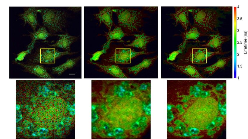
J. Phys. Photonics 2 (2020) 042005 https://doi.org/10.1088/2515-7647/abac1a
Journal of Physics: Photonics
TOPICAL REVIEW
Machine learning for faster and smarter fluorescence lifetime
OPEN ACCESS
imaging microscopy
RECEIVED
31 March 2020 Varun Mannam1, Yide Zhang1,2, Xiaotong Yuan1, Cara Ravasio1 and Scott S Howard1
REVISED 1
25 May 2020 Department of Electrical Engineering, University of Notre Dame, Notre Dame, IN 46556, United States of America
2
Caltech Optical Imaging Laboratory, Andrew and Peggy Cherng Department of Medical Engineering, California Institute of
ACCEPTED FOR PUBLICATION
4 August 2020 Technology, Pasadena, CA 91125, United States of America
PUBLISHED E-mail: showard@nd.edu
22 September 2020
Keywords: microscopy, fluorescence lifetime imaging microscopy, machine learning, convolutional neural network, deep learning,
classification, segmentation
Original Content from
this work may be used
under the terms of the
Creative Commons
Attribution 4.0 licence. Abstract
Any further distribution
Fluorescence lifetime imaging microscopy (FLIM) is a powerful technique in biomedical research
of this work must that uses the fluorophore decay rate to provide additional contrast in fluorescence microscopy.
maintain attribution to
the author(s) and the title However, at present, the calculation, analysis, and interpretation of FLIM is a complex, slow, and
of the work, journal
citation and DOI. computationally expensive process. Machine learning (ML) techniques are well suited to extract
and interpret measurements from multi-dimensional FLIM data sets with substantial
improvement in speed over conventional methods. In this topical review, we first discuss the basics
of FILM and ML. Second, we provide a summary of lifetime extraction strategies using ML and its
applications in classifying and segmenting FILM images with higher accuracy compared to
conventional methods. Finally, we discuss two potential directions to improve FLIM with ML with
proof of concept demonstrations.
1. Introduction
1.1. Motivation
Fluorescence microscopy is an essential tool in biological research that enables both structural and functional
molecular imaging of biological specimens [1]. Fluorescence lifetime imaging microscopy (FLIM) augments
fluorescence microscopy by measuring the effects of biological micro-environment on fluorescence decay
rate [2]. While powerful, extraction, and interpretation of the lifetime information is a complicated and
time-consuming process, as the raw FLIM data are multi-dimensional, and the FLIM algorithms are
computationally intensive.
Recently, machine learning (ML), particularly deep learning [3], has gained significant traction for its
excellent performance in processing complex multi-dimensional data. Whereas multiple ML methods have
been successfully utilized to extract fluorescence lifetime information, a comprehensive study of the ML
techniques applied to FLIM is still missing in the literature. In this topical review, we aim to fill this gap by
reviewing the articles reporting ML methods for FLIM applications. We also envisage two potential
applications of utilizing ML techniques to extract lifetime information with a small FLIM dataset.
1.2. Fluorescence microscopy
Fluorescence microscopy is one of the most powerful and versatile optical imaging techniques in modern
biology as it enables the study of cellular properties and dynamics in vitro and in vivo. Fluorescence
microscopy illuminates a specimen to excite fluorophores within cells and tissue and then collects the emitted
fluorescence light to generate images. To enhance contrast and identify specific features (like mitochondria),
fluorescence labeling can be introduced. Fluorescent labeling methods include genetic labeling using
fluorescent proteins [4], and chemical labeling by targeting species with antibodies [5]. By adequately
filtering the different wavelengths of the emitted light, the labeled features can be imaged and identified [1].
© 2020 The Author(s). Published by IOP Publishing Ltd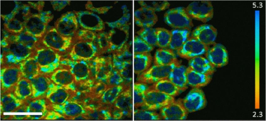
J. Phys. Photonics 2 (2020) 042005                                                                                      V Mannam et al

   Figure 1. Schematics of wide-field, confocal, two-photon, and light-sheet microscopes (CCD, charge-coupled device; PMT,
   photomultiplier tube; CL, cylindrical lens). Blue, red, and green light paths indicate UV (λ ≈ 400 nm) one-photon excitation, IR
   (λ ≈ 800 nm) two-photon excitation, and visible (λ ≈ 500 − 650 nm) fluorescence emission, respectively. Wide-field microscopy
   images the sample on to a focal point array. Pinhole blocks the out-of-focus light in confocal microscopy. Point-scanning confocal
   and two-photon microscopy scan a focused excitation spot within the sample. In light-sheet microscopy, excitation and emission
   are in orthogonal directions, and the sample field is imaged to a focal plane array.

     Fluorescence microscopy is commonly implemented in wide-field [6], confocal [7, 8], multi-photon
(two-photon) [9, 10], and light-sheet microscopy modalities [11] (figure 1). Wide-field microscopy achieves
high-speed imaging by simultaneously exciting fluorophores over a wide area and imaging the fluorescence
emission onto an imaging array (e.g. CCD camera). However, the wide-field microscopy images are typically
limited to surface or in vitro imaging as they cannot resolve depth and are susceptible to image blurring in
scattering tissue. Confocal microscopy overcomes this limitation by using a pinhole that is confocal with the
focal volume, thereby blocking the scattered light that would cause image blurring. However, such blocking
of light significantly reduces the signal to noise ratio (SNR) (and, therefore, speed) and imaging depth,
especially in highly scattering media. Multiphoton microscopy (MPM), in turn, improves imaging depth in
highly scattering media by exploiting the properties of non-linear optics to only excite fluorophores within a
diffraction-limited 3D volume in tissue and by collecting all emitted light without a pinhole. Since only
ballistic photons contribute to the non-linear optical excitation, MPM is resilient against the scattering of
excitation light. Recently, light-sheet microscopy has become a useful tool for high-speed, depth-resolved,
low-excitation level biological imaging by exciting a tissue cross-section and imaging the emission with an
imaging array. This approach gives exceptional results in cell culture and transparent organisms but
introduces technical limitations when employed in intravital imaging [12, 13].

1.3. Fluorescence lifetime imaging microscopy
The modalities in section 1.2 are fluorescence intensity-based techniques, which generate images by mapping
fluorophore concentration (emission) to position in the sample. In addition to fluorescence intensity
mapping, FLIM can provide additional information within the tissue compared to conventional
intensity-based methods. To understand what FLIM is measuring, we look to the fluorophore’s rate
equations. Figure 2 shows the Jablonski diagram illustrating the fluorescence generation process, where S0
and S1 are the ground and the first excited electronic states, respectively [2]. With the absorption of the
excitation light by the fluorescence molecule, the electrons are excited from S0 to S1 . The excited molecule
returns to S0 through a radiative (e.g. emitting fluorescence photons) or non-radiative (e.g. thermal
relaxation) spontaneous process, or through a stimulated emission process. When the fluorophore emission
is far below the fluorescence saturation emission rate, the spontaneous processes dominate and the
stimulated emission contributions can be ignored. The radiative decay rate is generally constant, while the
local micro-environment can modulate the non-radiative decay rate. The effective measured lifetime τeff is
therefore dependent on both the radiative lifetime τr and the non-radiative lifetime τnr The fluorescence
lifetime indicates the average time a fluorophore stays excited before relaxing and is typically in the range of
nanoseconds [7, 14].
     FLIM can be used to measure biologically important parameters such as ion concentrations, pH value,
refractive index [15], the dissolved gas concentrations [16–18], and about the micro-environment in the
living tissue [19–21]. Compared to conventional intensity-based fluorescence microscopy, FLIM is
independent of fluorophore concentration, excitation power, and photobleaching, which are extremely
difficult to control during most experiments [22]. Both fluorescence lifetime measurements and
conventional intensity imaging accuracy are limited by shot noise, and FLIM implementation method could

                                                       2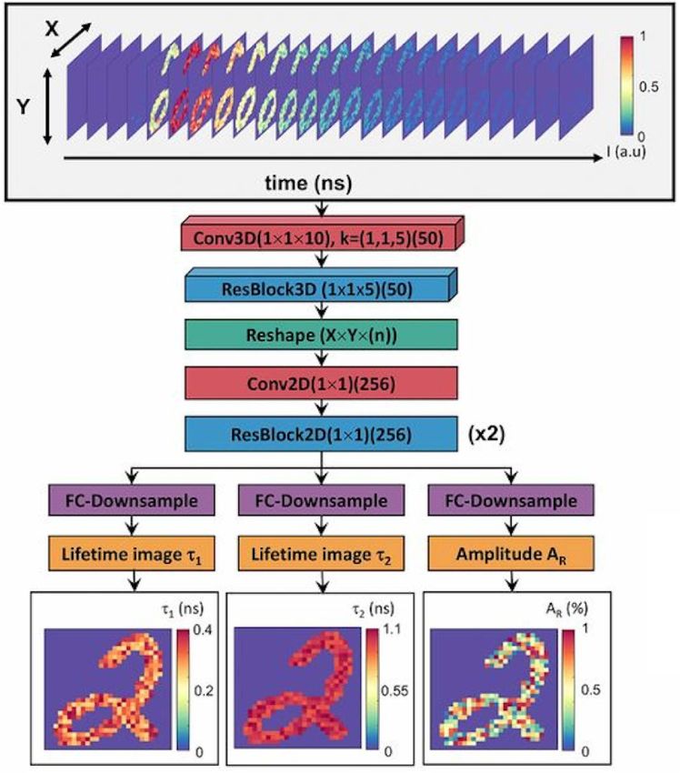
J. Phys. Photonics 2 (2020) 042005                                                                                         V Mannam et al

   Figure 2. Jablonski diagram of fluorescence process. Absorption and stimulated emission rates are a function of photon flux and
   drive fluorophore between ground and excited states. Radiative decay and non-radiative decay process are spontaneous and
   characterized by their decay lifetimes, τ. The radiative decay rate is considered a constant for a fluorophore and is represented by a
   solid line. The non-radiative decay rate is modulated by changes in the micro-environment and is represented with a dotted line.
   FLIM measurements commonly measure the effective decay rate, which is the sum of the radiative and non-radiative decay rates.

   Figure 3. Methods of fluorescence lifetime imaging microscopy. E(t) and F(t) are the excitation and emission signals, respectively.
   Left: time-domain FLIM implemented with time-gating; △t is the duration of the time gate, respectively. Right: frequency
   domain FLIM; ACE and ACF are the AC parts of the excitation and emission signals; M and △ϕ/ω are the modulation degree
   change and phase shift, respectively, of the emission with respect to the excitation.

further limit fluorescence lifetime measurement accuracy by reducing the ‘photon economy’ (i.e. the factor
that SNR is reduced from an ideal, shot noise limited system). However, FLIM photon economy can
approach the ideal shot noise limited SNR present in conventional intensity imaging when using time
domain or Dirac-pulse frequency domain implementations [23, 24]. Moreover, since the lifetime is an
intrinsic property of fluorescence molecules, FLIM is capable of separating fluorophores with overlapping
emission spectra, which cannot be distinguished by traditional intensity-based imaging methods provided
that there is a measurable difference in lifetime between the two fluorophores. Another application of FLIM
is Förster resonance energy transfer (FRET), which can measure the distance between donor and acceptor
molecules with 0.1 nm accuracy when within 10 nm of each other and with acceptable orientation [25–27].
FRET is extremely useful for applications such as protein studies in biological systems [28], dynamic
molecular events within living cells [29], and conformational changes in proteins [30].
    FLIM data is acquired through one of two general methods: time-domain (TD) FLIM, such as
time-correlated single-photon counting (TCSPC) [31] and time-gating (TG)[32]; and frequency-domain
(FD) FLIM [20, 33], as shown in figure 3 2. TD-FLIM methods measure the time between sample excitation
by a pulsed laser and the arrival of the emitted photon at the detector. FD-FLIM methods, on the other hand,
rely on the relative change in phase and modulation between the fluorescence emission and the periodically
modulated excitation to generate the lifetime images.

                                                        3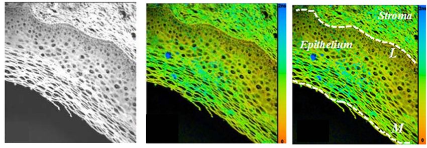
J. Phys. Photonics 2 (2020) 042005                                                                                           V Mannam et al

   Figure 4. NADH free/bound ratio mapping at different segments of a HeLa cell colony in a culture (taken on the 5th day of cell
   culture growth). The color coding reveals lower values of the a1 /a2 ratio for the cells at the center (left) and higher values for the
   cells at the edge (right) of a colony, possibly indicating higher and lower metabolic activities correspondingly. Scale bar: 100 µm.
   Data acquisition time: 700 s. [Adapted with permission from [34]. Copyright (2009) American Chemical Society.]

    In conventional TCSPC systems, the fluorescence lifetime is extracted from the measured fluorescence
intensity decay by fitting the experimental TCSPC signal as either a mono-exponential function or
multi-exponential function (for a mixture of fluorophores with different lifetimes). In a system consisting of
fluorophores with different lifetimes, an effective lifetime (τ) can be determined as the weighted average of
the independent lifetimes. The TCSPC signal (I(t)() is the convolution between the system’s instrument
response function (IRF) and the weighted sum of fluorescent decay paths, as shown in equation (1), where τn
and an are the lifetime and the corresponding weight of the n − th fluorophore population, respectively.
                                                                        ∑
                                                    I(t) = IRF(t) ∗           an e−t/τn .
                                                                          n

    Extracting lifetimes and their weights from multiple decay paths allows one to find the ratio
between two molecular populations with similar fluorescent emission spectra. For example, the
functional/conformational states of nicotinamide adenine dinucleotide reduced (NADH) can be used to
monitor oxidative phosphorylation, which is related to mitochondria oxidative stress [34]. Figure 4 shows
how fluorescence lifetime changes with different cellular metabolic states in the NADH; hence by measuring
fluorescence lifetime, one can extract the changes in the cellular metabolic state and thus accurately
characterize normal and pathological states. Figure 4 shows the extracted lifetime signal mapping by a
bi-exponential model in the commercial software SPCImage v2.8 [35]. Here, cells in the left section indicate
low a1 /a2 ratio values, and cells in the right section indicate higher a1 /a2 ratio values, which indicate higher
and lower metabolic activities, respectively.
    However, the extraction of fluorescence lifetime with curve-fitting using equation (1) in TD-FLIM data is
computationally slow, and long acquisition time is needed to build up statistical confidence [24] . On the
other hand, in time-gating FLIM systems (figure 3), the emission fluorescence intensity is integrated with
two or more time gates to extract the lifetime information of fluorophores with single or multiple
exponential decays. However, an accurate lifetime estimation requires a large number of time gates (8 or
more), which takes more time.
    The above issues in TD-FLIM can be fixed using FD-FLIM techniques. In FD-FLIM, the excitation light
is modulated at a frequency (ω), and the emission fluorescence has the same frequency but a decreased
amplitude and a shifted phase. Here, the amplitude modulation degree change is m, and the phase shift is ϕ
[21]. The lifetime in FD-FLIM can be extracted from either the amplitude change or the phase shift, which
are independent of fluorescence intensity and fluorophore concentration. In FD-FLIM, for fluorophores with
a single√exponential decay, the lifetimes (at the i−th pixel) calculated from the modulation degree change
(τm = 1/[m2i − 1]) and the phase shift (τϕ = tan(ϕi )/w) are identical [23]. For fluorophores of multiple
exponential decays, the lifetimes calculated from the modulation degree change or phase shift are weighted
averages of individual lifetime values.
    To simplify the interpretation and visualization of lifetime information, phasor plots can be used with
raw TD- and FD-FLIM data [36]. As an example, figure 5 shows a simple phasor plot with two lifetime decays

                                                         4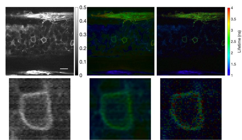
J. Phys. Photonics 2 (2020) 042005                                                                         V Mannam et al

                                     Figure 5. Phasor plot for fluorophores with two exponential decays.

τ1 (short lifetime) and τ2 (long lifetime) and their weighted average. Phasor analysis is also useful analyzing
molecules with multi-exponential decays, such as in commonly used FRET donor fluorophores [37–41].
     Phasor plots are 2D representations of lifetime information, where the short lifetime is on the right side
of the semi-circle, and the long lifetime is on the left. The coordinates along the x-axis (G) and y-axis (S)
represent the real and imaginary values, respectively, of the phasor extracted from raw FLIM data. The two
extremes of the semi-circle represent 0 and ∞ lifetimes with coordinates (1, 0) and (0, 0), respectively. For
fluorophores with a single exponential decay, the phasor always lies on the semi-circle. For fluorophores with
two exponential decays, the phasor lies on the line connecting the phasors corresponding to individual
lifetimes. Similarly, for fluorophores with three exponential decays, the phasor is inside the triangle
connecting all the three individual phasors.
     The phasor plot is obtained using either TD-´ or FD-FLIM raw data   ´ ∞ [42]. For TCSPC data, the phasors
                                                      ∞
can be´∞acquired  using  the
                          ´∞ transformations  g i =  0
                                                        I(t) cos(wt)dt/   0
                                                                             I(t)dt and
si = 0 I(t) sin(wt)dt/ 0 I(t)dt, where gi and si are the coordinates along the G and S axes, respectively, w is
the modulation frequency, and I(t)( is the TCSPC data at the i−th pixel. For FD-FLIM data, the phasors can
be calculated using gi = mi cos(ϕi ), si = mi sin(ϕi ), where gi and si are the phasor coordinates, mi and ϕi are
the modulation degree change and the phase shift of the emission with respect to the excitation at the i−th
pixel. Regardless of whether the phasors are generated from TD-FLIM or FD-FLIM setups, the phasor
                                                   ∑n                                ∑n
coordinates are related to the lifetimes by gi = k=1 ak,i /[1 + (wτk )2 ] and si = k=1 ak,i wτk /[1 + (wτk )2 ],
where ak,i, is the intensity-weighted fractional contribution of the k−th fluorophore with lifetime τi at the
                 ∑n
i−th pixel and k=1 ak,i = 1 [43]. The average lifetime at the i−th pixel is defined as the ratio of si and gi
with an additional factor of ω1 .
     Extraction of the fluorescence lifetime using the curve-fitting techniques is a complex process, and
different software solutions are provided by different vendors [35, 44–52]. All of these tools are
computationally inefficient for real-time measurements. Many FLIM applications like FRET are quantitative
and require data analysis in multiple dimensions, which can be overwhelming for existing software solutions
mentioned above. To address these problems, we consider ML as one of the potential choices. ML is also
helpful in interpreting the complex data and extracting the multi-dimensional data to a single exponent
lifetime. The following sections will discuss the basic ideas and lifetime applications with ML.

1.4. Machine learning
Computing and interpreting TD-FLIM and FD-FLIM is computationally complex, slow, and leads to
challenges in extracting biological interpretation from the raw data. ML approaches can be applied to
accelerate imaging and aid interpretation significantly. Recently there has been a significant development in
the processing of imaging techniques that mainly rely on ML methods. The ML methods have been
extensively used in image processing and are model-free. A subset of ML is artificial neural networks (ANNs)
that are inspired by biological neural networks and provide robust performance in applications such as
systems identification and control [53], classification, and medical image analysis [54]. In medical image
processing, ANN plays a vital role in the classification and segmentation of pre-cancer cells, resolution
enhancement in histopathology [55], super-resolution microscopy [56], fluorescence signal prediction from
label-free images [57], fluorescence microscopy image restoration [58], and hyperspectral single-pixel
lifetime imaging [59].

                                                         5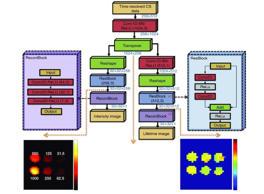
J. Phys. Photonics 2 (2020) 042005                                                                                    V Mannam et al

   Figure 6. Overview of FLIM approaches using ML: (a) raw data, (b) fluorescence lifetime image, and (c) lifetime image segmented
   with an ML approach. Solid line indicates conventional FLIM processing data flow; dashed line indicates ML FLIM processing
   data flow. In this flow chart, the ML block can include combinations of FC layers, CNNs, and unsupervised learning techniques
   for different applications, as described in the text. Microscope images are of intrinsic fluorophore imaging in an in vivo mouse
   kidney [43]. Scale bar: 20 µm.

    In particular, deep neural networks (DNNs), a subset of ANN that uses a cascade of layers for feature
extraction [3], mainly fully connected (FC) networks and convolutional neural networks (CNNs), have made
significant progress in various imaging tasks such as classification, object detection, and image
reconstruction.
    ML approaches have achieved unprecedented results; however, a few challenges are associated with them.
First, the data-driven ML model requires a large training dataset, and such datasets are difficult to acquire.
Second, training the ML model takes a significant amount of time (typically hours or days) and substantial
resources (like high-performance graphical processing units).

2. Overview of FLIM approaches using ML

In this section, we consider publications that address fluorescence lifetime and its applications using machine
learning. We divide the research articles into two main categories. First, those focusing on estimation of
lifetime from input data (either in TD or FD) using ML. Second, those exploring the lifetime applications
such as classification, segmentation using ML.
     Figure 6 indicates the flow diagram of FLIM measurements using ML in a step-by-step process. First, the
raw FLIM data is acquired using a TD- or FD-FLIM system. Second, the lifetime can be extracted from either
TD- or FD-FLIM measurements. In the time-domain, for each pixel, a histogram of the number of emitted
photons is processed using curve fitting methods to estimate the lifetime parameters (lifetime values τn and
their weights an , as in equation (1)). However, time-domain measurements (per-pixel) with curve fittings are
computationally expensive and are not suitable for real-time measurements. Instead, one can efficiently
solve for lifetime using ML methods. Similarly, ML methods can be used to estimate lifetime from TD
measurements of the complete 3D stack (x, y, t, , ). Another way to process this per-pixel histogram is by
using phasors to get the average lifetime (τavg ). In the frequency-domain, for each-pixel, changes in the
modulation degree m and phase ϕ are measured to calculate single exponent lifetime τ. For multi-exponent
lifetime values, τavg can be estimated (for each-pixel) using the phasor approach. Lifetime estimation from
input data using ML is discussed in section 3.
     Once the lifetime image is available, applications like classification and segmentation can be applied.
Typical classification applications can be performed using basic statistics (mean and variance) on the lifetime.
However, a threshold lifetime is required to classify lifetime images from these statistics. If training data is
available, then a data-driven model can be employed to perform the same classification using ML methods.
Classification and segmentation from lifetime using ML are discussed in sections 4 and 5, respectively.
Potential applications of lifetime information with ML and their proofs of concept are discussed in section 6.

                                                      6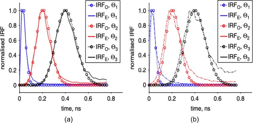
J. Phys. Photonics 2 (2020) 042005                                                                                       V Mannam et al

   Figure 7. (a) Intensity image, (b) short lifetime τF image generated by ANN and, (c) merged intensity and average lifetime τAverage
   image of daisy pollens [60].

3. Estimation of FLIM images using ML

ML is well suited for estimating per-pixel fluorescence lifetime measurements from raw-data. Fluorescence
lifetime can be estimated from TD-FLIM raw-data without computationally expensive curve fitting methods
by using an artificial neural network (ANN) [60].
     Wu et al used an ANN is used to approximate the function that maps TCSPC raw data as input onto the
unknown lifetime parameters in [60]; figure 7 displays this method applied to daisy pollens. Here an ANN
model with two-hidden fully connected (FC) layers is trained with the TCSPC raw data from each pixel as
input and its corresponding lifetimes (short and long lifetimes) and weights of the lifetime ratio as outputs.
Figure 7(a) shows the intensity of a daisy pollen in terms of photon count, and figure 7(b) shows the
extracted short lifetime (τF) using the trained ANN for the complete image. The estimation of the lifetime
image (size of 256 × 256) with the ANN method takes only 0.9 s, which is 180 times faster than the
least-squares method (LSM) based curve-fitting technique, which takes 166 s. The weighted average of short
and long lifetime results in an average lifetime image. The merged image of intensity and the average lifetime
is shown in figure 7(c), where intensity and the fluorescence lifetimes are mapped to the pixels’ brightness
and hue, respectively. From [60] it was also observed that the LSM method failed to estimate the accurate
lifetime parameters due to its sensitivity to initial conditions. The success rate for estimating accurate lifetime
parameters with the ANN method was 99.93%, and the LSM method was 95.93%, which shows that the
ANN method has improved estimation accuracy of lifetime from the TCSPC raw data compared to curve
fitting tools [60].
     Another area where ML can improve data analysis/computing efficiency is estimating lifetime from a
TCSPC system, including an IRF. For a TCSPC system, IRF must be measured throughout a set of FLIM
measurements to account for variations in pulse shape during the experiment. The deconvolution of IRF
with TCSPC data provides lifetime information. However, measuring IRF requires additional steps before
performing FLIM measurements. Many lifetime analysis tools ignore the IRF and use tail-fitting for
estimation of a lifetime. ML can estimate the instrument response function IRF(t) in addition to single
exponent lifetime τ from the TCSPC histogram data at every pixel with the Expectation-Maximization (EM)
algorithm [61]. Gao et al demonstrated the EM to estimate the model parameters τ and IRF in [61]. The
input to EM is the histogram of TCSPC data, and the output is lifetime and IRF. Figure 8 illustrates the
results for the estimation of lifetime and IRF for different configurations. Thus, Gao and Li [61] show that
the IRF profiles could be extracted accurately using the EM method.
     As we have seen, extracting lifetime from TCSPC data for each pixel is computationally inefficient even
when applying ML approaches. Therefore, implementing ML techniques for 3D data (x, y, t, , ) is challenging.
Recently, Smith, et al proposed a novel method for estimating lifetime parameters on the complete 3D
TCSPC dataset using convolutional neural networks (CNNs) in [62]. In [62], the 3D CNN is trained using a
synthetic data generator (from MNIST: handwritten digits dataset [63]) to reconstruct the lifetime images
(τ1 and τ2). In this network, input data is the spatial and time-resolved fluorescence decays as a 3D data-cube
(x, y, t, , ).
     Figure 9 shows the architecture of fluorescence lifetime imaging-network (FLI-Net), which consists of a
common branch for temporal feature extraction and subsequent split branches for the reconstruction of
lifetimes (short τ1 and long τ2) and fractional amplitude of the short lifetime (AR ). In this architecture, the 3D
convolutions (Conv3D) along the temporal dimension at each spatially located pixel are considered to
maximize spatially independent feature extraction along with each temporal point spread function (TPSF).
The use of a Conv3D layer with a kernel (which is a learning parameter during training) size of 1 × 1 × 10
reduces the potential introduction of unwanted artifacts from neighboring pixel information in the spatial

                                                       7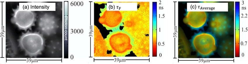
J. Phys. Photonics 2 (2020) 042005                                                                                     V Mannam et al

   Figure 8. Comparison of estimated IRF (IRFE ) and original IRF (IRFO ) with different lifetime (a) τ = 0.5 ns and (b) τ = 1.5 ns.
   The full widths at half maximum of IRFs, Θ where Θ1 , Θ2 , and Θ3 are 50 ps, 150 ps, and 200 ps respectively (Reuse permission is
   taken from the author [61]).

dimensions (x and y) during training and inference. Then a residual block (ResBlock) of reduced kernel
length enables the further extraction of temporal information. After resolving the common features of the
whole input, the network splits into three dedicated convolutional branches to estimate the individual
lifetime-based parameters. In each of these branches, a sequence of convolutions is employed for
down-sampling to the intended 2D image (short or long lifetime). Finally, Smith et al [62] compared the
results obtained from FLI-Net and the conventional least-squares fitting (LSF) method and observed that
FLI-Net is accurate.
     Thus, we can solve a 3D CNN problem with TCSPC 3D data (x, y, t, , ) as input and lifetime parameters as
output, but memory is still a major challenge that must be addressed. During the training of this ML model
with a TCSPC raw data, more memory (due to a large number of parameters) is required, which makes it
difficult to process with a limited memory system. Performing image processing with massive data will be
more challenging to perform in real-time; if the data is a 3D stack (x, y, z, , ). For example, an image of size
256 × 256, with 256 time-resolved bins, each containing 10 bits (maximum value is 1023), has a size of
20.97 MB and if the data is a 3D stack (x, y, z, , ), then the total size is in GB. To remedy this, Yao, et al
combined compressive sensing (CS) with a deep learning framework to efficiently train the model in [59].
     In the CS approach, the input image data I are related with compressive patterns (like Hadamard
patterns P) such that PI = S, where S is the CS data collected with patterns P. In this case, the intensity images
are recovered using the CS-based inverse-solvers for each time gate, and the lifetime images are
recovered using either curve-fitting tools or ML from the time-resolved intensity images. In multi-channel
(different-wavelengths) CS data, the above procedure repeats for each channel. In [59], the authors provide a
ML architecture that extracts the intensity and lifetime images from the time-resolved CS data, as shown in
figure 10. This architecture is defined as Net-FLICS (fluorescence lifetime imaging with compressive sensing
data). Net-FLICS is a combination of two network designs: ReconNet [64] and Residual Network (ResNet)
[65]. The ReconNet is useful to reconstruct intensity images from random single-pixel measurements.
ResNet is composed of one fully connected layer and six convolutional layers. Net-FLICS takes an array of
size 256 × 512 as the input, which represents 512 CS measurements with 256 time gates, and outputs an
intensity image and a lifetime image, both of which have sizes of 32 × 32, as the reconstruction prediction.
     In summary, Net-FLICS contains three main segments: (1) a shared segment that recovers the sparsity
information from CS measurements; the first segment output represents the temporal point spread functions
(TPSF) of each pixel; (2) an intensity reconstruction segment that contains one ResBlock and one
ReconBlock; (3) a lifetime reconstruction segment that contains a 1D convolutional layer, two ResBlocks,
and two ReconBlocks. Figure 10 shows the estimated intensity and lifetime from time-resolved CS data of
Alexa Fluor dye (AF750, ThermoFisher Scientific, A33 085), which is pH-insensitive over a wide molar range,
for stable signals in imaging with six different concentrations starting from 1000 nM to 31.25 nM. The mean
lifetime of the dye is 0.5 ns. As the concentration reduces, the number of detected photons also decreases. In
the next section, we will explore the lifetime applications, like classification with ML.

                                                      8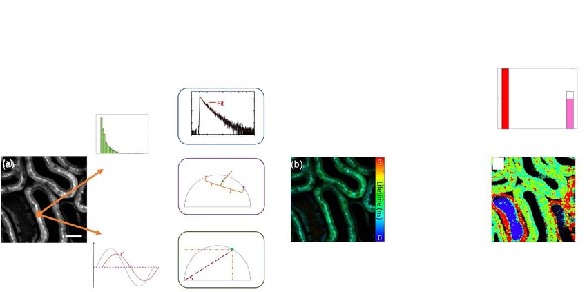
J. Phys. Photonics 2 (2020) 042005                                                                                         V Mannam et al

   Figure 9. Illustration of the 3D-CNN FLI-Net structure. During the training phase, the input to neural network was a set of
   simulated data voxels (which is the 3D data (x, y, t, , )) containing a TPSF at every nonzero value of a randomly chosen MNIST
   image. After a series of spatially independent 3D convolutions, the voxel underwent a reshape (from 4D to 3D) and is
   subsequently branched into three separate series of fully convolutional down-sampling for simultaneous spatially resolved
   quantification of 3 parameters, including short lifetime (τ1), long lifetime (τ2), and amplitude of the short lifetime (AR ) (Reuse
   permission is taken from the author [62]).

4. FLIM applications using ML: Classification

In this section, we enumerate the lifetime applications, surrounding classification of cells using ML. One
application of lifetime is classifying pre-implantation mouse embryos’ metabolic states as healthy or
unhealthy. This estimation of embryo quality is especially helpful for in vitro fertilization (IVF) [66]. Health
monitoring can be achieved via invasive and non-invasive methods, but non-invasive methods significantly
reduce the time and human resources necessary for analysis compared to invasive methods. Thus, estimating
the quality of embryos using non-invasive methods is preferable, and extraction of lifetime information is an
important step in these methods. In this non-invasive method, lifetime information is extracted from
embryos at different time steps to monitor the cell culture at every stage. This lifetime information,
combined with a phasor plot, shows embryos’ growth in a specific way. Ma et al demonstrated the phasor
plot at different time steps of embryos correlates with embryonic development, and this phasor trajectory is
called a development trajectory in [66]. Here, the lifetime trajectory reveals the metabolic states of embryos.
    With the ML algorithm, the trajectory of embryo health can be identified at an early stage by using a
phasor plot of early samples. The ML algorithm is called distance analysis (DA) [67], and it outputs the
embryo viability index. In the DA algorithm [67], the phasor plot is divided into four equidistance
quadrants, and in each quadrant, a few statistics are measured (see [67] for details). Finally, the measured
statistics are used to identify healthy and unhealthy results. Based on the embryos viability index (EVI) from
the DA algorithm, the embryo classifies as either healthy or unhealthy.

                                                        9
J. Phys. Photonics 2 (2020) 042005 V Mannam et al
Figure 10. The architecture of Net-FLICS and outputs at different endpoints of Net-FLICS (intensity and lifetime). Intensity and
lifetime for the decreasing AF750 concentration from 1000 nM to 31.5 nM in six steps with true lifetime of 0.5 ns [59].
Figure 11. Schematic of FLIM-Distance Analysis Pipeline to classify the mouse embryos. Scale bar: 100 µm [66].
Figure 11 shows the flowchart for classification of the early-stage mouse embryos [66]. First, embryos are
collected at 1.5, 2.0, 3.0, 3.5, and 4.5 days post-fertilization and identified as 2-cell, Morula, Compaction,
Early Blastocyst and, Blastocyst, respectively. Second, at the Compaction stage, the intensity image is passed
through the FLIM setup to get the lifetime image. Here, lifetime information is generated using Compaction
stage TCSPC data. Third, the generated phasor plot is passed through the DA algorithm to get the EVI.
Finally, the Compaction stage embryo is classified based on its EVI. For the healthy (H) embryos, the EVI
value is less than zero, and for the unhealthy (UH) embryos, the EVI value is greater than zero. Figure 11
shows one healthy and one unhealthy embryo Blastocyst image identified by using the non-invasive lifetime
and phasor approach with ML.
ML can also be used to improve the quantitative diagnosis of precancer cells with lifetime information.
For example, Carcinoma of the uterine cervix is the second-largest cause of cancer in women worldwide and
is responsible for thousands of deaths annually [68]. Gu et al imaged cervical tissue cells (a combination of
the stroma and epithelium regions) using a fluorescence lifetime setup in [69]. Here the TCSPC data is
captured, and lifetime information is extracted with a double exponent model at each pixel using SPCImage
software. The extracted cells are classified as normal or cervical intraepithelial neoplasia (CIN) stage cells
(from stage 1 to stage3) based on their lifetime information. Out of these normal cells, CIN1 stage cells are
10J. Phys. Photonics 2 (2020) 042005 V Mannam et al
Figure 12. Fluorescence (a) intensity and (b) lifetime images of a typical H & E stained normal cervical tissue section. The region
towards the right is the stroma, while the region on the left is the cell-rich epithelium separated by a visible boundary. (c) Lifetime
images with markers where the basement membrane was marked out by white dashed line L and epithelium surface was
delineated by white dashed line M [69, 70]. The color bars in (b), and (c) represent fluorescence lifetime on a scale of 0 (red) to 2
ns (blue). Scale bar: 100 µm.
considered to be low-risk cells, while CIN2 and CIN3 stage cells are considered to be high-risk cells.
A typical hematoxylin and eosin (H & E) stained normal cervical tissue section is shown in figure 12.
In these cells, stroma and epithelium regions are marked, as shown in figure 12(c). In [69], the longer
lifetime (τ2 ) statistics (mean and standard deviation) of the epithelium region are calculated and considered
as feature vectors of the ML model. In the model, lifetime feature vectors are passed through a single hidden
layer neural network to classify the cells using extreme learning machine (ELM) algorithm [71]. ELM can
accurately identify precancer cells in the epithelium region, and it can accurately classify precancer cells as
low or high risk. Gu et al separated the epithelium region into multiple layers, and each layer’s feature vectors
are measured in [70]. At each layer, feature vectors are used for classification with the ELM algorithm, to
observe more accurate results. The mean lifetime of each layer is higher than the previous layer for normal
cells, and for the precancer cells, the difference observed between each successive layer is less than in the
healthy cells. In the next section, lifetime information applied to segmentation with ML is explained.
5. FLIM applications using ML: Segmentation
In this section, we explore another application of FLIM, segmentation of cells using ML. In a given lifetime
image containing two or more cells, it is essential to identify the locations of these cells and group them based
on their lifetime values. However, measured lifetime at a pixel is an average value, and it cannot resolve the
heterogeneity of fluorophores at that pixel since different fluorophore compositions (single fluorophore,
multiple fluorophores) or excited state reactions could result in the same average lifetime measurements.
Fortunately, different fluorophore compositions and possible excited state reactions can alter the phasor
coordinates even if the average lifetime might be unchanged; therefore, the heterogeneity of fluorophores can
be resolved with the phasor approach.
In the phasor plot, pixels with similar fluorescence decays group together. This feature is useful for
segmenting pixels based on the similarity of their fluorescence decays. Therefore, the lifetime segmentation
technique is simplified using phasors by selecting adjacent phasor points and labeling them with different
colors. However, this technique often leads to biased results.
Zhang et al demonstrated an unbiased method to segment the lifetime image using K-means clustering,
an unsupervised ML algorithm in [43]. Figure 13(a) shows the lifetime image of a living mouse kidney
captured using our custom-built two-photon microscope [72] and figure 13(b) shows its phasor. By giving
an estimated number, K, of different fluorophores present in the image, this approach separates its phasor
plot into K clusters using the K-means clustering algorithm. K-means clustering on the phasors shown in
figure 13(b) with four clusters is shown in figure 13(c). The segmented lifetime image for each cluster with a
different color in figure 13(d) represents the different proximal tubules (S1 and S2 ) in the cells. K-means
clustering technique is useful for segmenting phasors into groups without any bias. This segmentation
method provides more consistent segmentation results and applies to both fixed and intravital 2D and 3D
images. In the next section, the potential directions of FLIM using ML as well as their proofs of concept are
discussed.
11J. Phys. Photonics 2 (2020) 042005 V Mannam et al
Figure 13. Two-photon fluorescence lifetime image (a), phasor plot (b), K-means clustering on phasors (c), and segmented
lifetime (d) of the kidney in a living mouse. Scale bar: 20 µm. Adapted with permission from [43] @ The Optical Socity.
6. Potential directions
The aforementioned ML-based FLIM applications (classification and segmentation) outperform
conventional methods in terms of accuracy and computational time. Implementing ML techniques on
fluorescence microscopy images has opened a considerable potential for research in the field of biomedical
image processing. However, the potential uses of ML are not limited to the previously described techniques.
To describe potential future directions, we demonstrate two proof-of-concept implementations of ML in
FLIM for novel techniques. First, we demonstrate a framework for denoising fluorescence lifetime images
using ML. Second, we illustrate estimating fluorescence lifetime images from conventional fluorescence
intensity images.
6.1. Denoising of FLIM images using ML
According to section 2, it is clear that lifetime information is critical for classification and segmentation
applications. However, the lifetime image (τ) is noisy as it is obtained from the noisy raw data I(t)(.
Therefore, one of the future directions of the field is to perform fluorescence lifetime denoising using ML,
similar to our previous fluorescence microscopy intensity denoising [73]. After the noise in the lifetime is
reduced, the accuracy of classification and segmentation will increase.
In [43], the lifetime is defined as the ratio of S and G (with an additional factor of ω1 ) at lock-in
(modulation) frequency. Hence we can consider denoising SS and GG images separately, and the denoised
lifetime becomes Ŝ/(Ĝw), where Ŝ and Ĝ are the denoised S and G, respectively. We observe that denoising S
and G images independently provide better results compared to direct denoising of lifetime images.
For image denoising, there are several methods proposed. One of the methods was discussed in our
previous paper [73] to perform fluorescence intensity denoising using ‘Noise2Noise’ convolutional neural
network for the mixture of Poisson-Gaussian noise. In [73], image denoising with ML outperforms all the
existing denoising methods in two areas: accuracy (around 7.5 dB improvement in peak signal-to-noise ratio
(PSNR)) and test time, which is less than 3 seconds using a central processing unit (CPU). The accuracy
obtained in [73] is better since the ML model was trained with confocal, two-photon, and wide-field
microscopic modalities which provide the most generalized model that can solve the denoising of Poisson
noise, Gaussian noise, and a mixture of both.
12J. Phys. Photonics 2 (2020) 042005 V Mannam et al
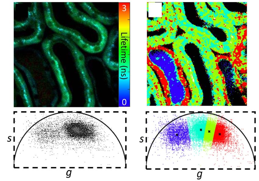
Figure 14. Fluorescence lifetime denoising using ML. From left to right: noisy composite lifetime, denoised composite lifetime,
target composite lifetime. Composite lifetime is the hue saturation value (HSV) representation of intensity and lifetime images
together, where intensity and the fluorescence lifetimes are mapped to the pixels’ brightness and hue, respectively. The top row
indicates a field of view (FOV) of 512 × 512 size, and the bottom row shows the region of interest (ROI) from the FOV (as shown
in the yellow box) of size 100 × 100. The selected ROI indicates nuclei and mitochondria in green and light-blue colors,
respectively. Scale bar: 20 µm.
In this work, we implement the same Noise2Noise pre-trained model (trained for fluorescence intensity
images) [73] to denoise the S and G images separately and obtain Ŝ and Ĝ. In figure 14 the denoised lifetime
image is similar to the target image (where target lifetime is generated by averaging 50 noisy lifetime images
within the same FOV) and much better than the noisy lifetime image. Raw lifetime images are captured with
our custom-built two-photon microscope FLIM setup [72] with an excitation wavelength of 800 nm, an
image dimension of 512 × 512, the pixel dwell time of 12 µs and pixel width of 500 nm. The samples we used
are fixed BPAE cells [labeled with MitoTracker Red CMXRos (mitochondria), Alexa Fluor 488 phalloidin
(F-actin), and DAPI (nuclei)] from Invitrogen FluoCells F36924.
In figure 14, the noisy lifetime is generated from the noisy S and G images. These S and G images are
passed through a pre-trained model in a plugin we developed for ImageJ [74] to get Ŝ and Ĝ images. The
denoised lifetime is the ratio of Ŝ and Ĝ. The improvement in PSNR in the denoised lifetime image is 8.26 dB
compared to the noisy input lifetime image, which is equal to the average of 8 noisy images (in the same
FOV)-thereby reducing the computation time by eight folds, instead of averaging more lifetime images for a
better SNR. The denoised lifetime image (with high SNR) provides higher accuracy for classification and
segmentation tasks. This work is a proof of concept for denoising lifetime images using a pre-trained model.
If one is interested in obtaining better accuracy, the neural network has to be trained from scratch, which
needs a large number of raw lifetime images as training data. As the acquisition of a large number of lifetime
images is time-consuming, we show here the proof of concept using limited images and a pre-trained model.
6.2. Estimation of FLIM images from intensity images using ML
In section 1.3, the estimation of lifetime using either TD or FD techniques is computationally expensive and
requires additional hardware. One can construct a model with ML that reduces the computational time
significantly. However, the ML model requires additional information such as the photon count histogram in
TD or phase information in FD. The required hardware setup for acquiring this additional information is
expensive for many research labs. To address this issue, we propose another potential future direction to
estimate fluorescence lifetime images from conventional fluorescence intensity images without either TD or
FD setup. If one has a large training dataset (intensity and lifetime images), then a neural network model can
be trained that maps the intensity to lifetime accurately.
As a proof of concept, in this section, we demonstrate the advantage of using machine learning for the
estimation of fluorescence lifetime from a conventional intensity image using a limited training dataset and a
specific biological model. In this work, we acquired a small dataset (intensity and lifetime image pairs) of a
zebrafish that was two days post-fertilization and labeled with enhanced green fluorescence protein (EGFP
13J. Phys. Photonics 2 (2020) 042005 V Mannam et al
Figure 15. Estimation of fluorescence lifetime from intensity using ML. From left to right: raw intensity image, estimated
composite lifetime, target composite lifetime. Composite lifetime is the HSV representation of intensity and lifetime images
together, where intensity and the fluorescence lifetimes are mapped to the pixels’ brightness and hue, respectively. The top row
indicates the field of view (FOV) of size 360 × 360, and the bottom row indicates the region of interest (ROI) from the FOV (as
shown in the yellow box) of size 50 × 50. Scale bar: 10 µm.
labeled transgenic (Tg): sox10 megfp). The dataset size we use for training the network is 140 images, and the
test data contains 16 images. Images in this in vivo dataset were captured with our custom-built two-photon
microscope [72] at different wavelengths and power levels to generalize the model. Thus, we train a NN
model that maps the zebrafish intensity to zebrafish lifetime values.
The estimated lifetime closely matches the target lifetime with a structural similarity index (SSIM) [75]
of 0.902 3, where SSIM value close to 1 indicates that the model prediction is good and also shows how close
the estimated and target images are matched. Here, we consider a famous neural network architecture
(U-Net: which consists of an encoder and decoder structure [76]) with an input of 256 × 256, encoded to the
latent space of 8 × 8, and reconstructed back to a lifetime image of 256 × 256. We consider two training
models with the target for one model to be lifetime and the target for the other model to be a composite
lifetime. Here, composite lifetime is the HSV representation of intensity and lifetime images together, where
intensity and the lifetimes are mapped to the pixels’ brightness and hue, respectively. We observe that the best
lifetime estimation from intensity results occur when the composite lifetime, rather than the lifetime itself, is
the target. Therefore, we choose the composite lifetime as the target to train our model.
The model that we present has certain limitations. First, a large amount of data is required to train the
model as lifetime information is unique to each molecule, and the trained model requires a massive
collection of lifetime and intensity image pairs. Second, the model behaves differently for stained and
unstained samples since intensity is mapped to a lifetime in the stained samples that are different, and
therefore incorrect, in the unstained samples. Finally, retraining the NN takes more computational time and
resources; therefore, in this work, we show a proof of concept with a limited image dataset and retrained NN
model, as in figure 15.
7. Conclusions
In this topical review, we have summarized the conventional lifetime extraction methods using both TD- and
FD-FLIM techniques. Since the extraction of lifetime images is a complex process, ML stands out as a viable
alternative to extract the lifetime at a faster rate with high accuracy. We have reviewed the novel applications
of ML techniques to FLIM, such as a network for fluorescence lifetime imaging using compressive sensing
data (Net-FLICS) and a 3D CNN fluorescence lifetime imaging network (FLI-Net) used for the lifetime
extraction. Also, we have reviewed the applications of lifetime images such as classification and segmentation
using novel ML techniques, including distance analysis (DA), extreme learning machine (ELM), and
14J. Phys. Photonics 2 (2020) 042005 V Mannam et al
K-means clustering. Here, we have shown that the application of ML in FLIM significantly improves the
computational speed and accuracy of the lifetime results.
Finally, we have proposed two additional potential directions for FLIM using ML approaches, including
the denoising of fluorescence lifetime images and the estimation of lifetime images from conventional
fluorescence intensity images. Both directions are presented with proofs of concept using datasets with a
limited size. Our results demonstrate that ML can be one of the potential choices for future applications
of lifetime images. For example, with a large dataset, a generalized model can be generated for the extraction
of lifetime images from conventional fluorescence intensity images that significantly reduces the cost of a
FLIM setup.
Disclosures
The authors declare no conflicts of interest.
Funding information
This material is based upon work supported by the National Science Foundation (NSF) under Grant No.
CBET-1554 516.
Acknowledgment
Yide Zhang’s research was supported by the Berry Family Foundation Graduate Fellowship of Advanced
Diagnostics & Therapeutics (AD&T), University of Notre Dame. The authors acknowledge the Notre Dame
Integrated Imaging Facility (NDIIF) for the use of the Nikon A1R-MP confocal microscope and Nikon
Eclipse 90i widefield microscope in NDIIF’s Optical Microscopy Core. The authors further acknowledge the
Notre Dame Center for Research Computing (CRC) for providing the Nvidia GeForce GTX 1080-Ti GPU
resources for training the neural networks using the Fluorescence Microscopy Denoising (FMD) dataset in
TensorFlow.
ORCID iDs
Varun Mannam https://orcid.org/0000-0002-1866-6092
Yide Zhang https://orcid.org/0000-0002-9463-3970
Scott S Howard https://orcid.org/0000-0003-3246-6799
References
[1] Lichtman J W and Conchello Je-A 2005 Fluorescence microscopy Nat. Methods 2 910–9
[2] Chang C-W, Sud D and Mycek M-A 2007 Fluorescence lifetime imaging microscopy Methods Cell. Biol. 81 495–524
[3] Goodfellow I, Bengio Y and Courville A 2016 Deep Learning (Cambridge, MA: MIT Press) http://www.deeplearningbook.org
[4] Day R N and Schaufele F 2008 Fluorescent protein tools for studying protein dynamics in living cells: a review J. Biomed. Opt.
13 031202
[5] Sahoo H 2012 Fluorescent labeling techniques in biomolecules: a flashback RSC Adv. 2 7017–29
[6] Verveer P J, Gemkow M J and Jovin T M 1999 A comparison of image restoration approaches applied to three-dimensional
confocal and wide-field fluorescence microscopy J. Microsc. 193 50–61
[7] Pawley J 2010 Handbook of Biological Confocal Microscopy (Berlin: Springer) (https://doi.org/10.1007/978-0-387-45524-2)
[8] Semwogerere D and Weeks E R 2005 Confocal microscopy Encyclopedia of Biomaterials and Biomedical Engineering (Boca Raton,
FL: CRC Press) (https://doi.org/10.1201/9780429154065)
[9] Hoover E E and Squier J A 2013 Advances in multiphoton microscopy technology Nat. Photon. 7 93–101
[10] Zipfel W R, Williams R M and Webb W W 2003 Nonlinear magic: multiphoton microscopy in the biosciences Nat. Biotechnol.
21 1369–77
[11] Santi P A 2011 Light sheet fluorescence microscopy: a review J. Histochem. Cytochem. 59 129–38
[12] Bouchard M B, Voleti V, Mendes Cesar S, Lacefield C, Grueber W B, Mann R S, Bruno R M and Hillman E M C 2015 Swept
confocally-aligned planar excitation (SCAPE) microscopy for high-speed volumetric imaging of behaving organisms Nat. Photon.
9 113
[13] (https://andrewgyork.github.io/high_na_single_objective_lightsheet/)
[14] Berezin M Y and Achilefu S 2010 Fluorescence lifetime measurements and biological imaging Chem. Rev. 110 2641–84
[15] Won Y J, Han W-T and Kim D Y 2011 Precision and accuracy of the analog mean-delay method for high-speed fluorescence
lifetime measurement J. Opt. Soc. Am. A 28 2026–32
[16] Khan A A, Fullerton-Shirey S K and Howard S S 2014 Easily prepared ruthenium-complex nanomicelle probes for two-photon
quantitative imaging of oxygen in aqueous media RSC Adv. 5 291–300
[17] Khan A A, Vigil G D, Zhang Y, Fullerton-Shirey S K and Howard S S 2017 Silica-coated ruthenium-complex nanoprobes for
two-photon oxygen microscopy in biological media Opt. Mater. Exp. 7 1066–76
[18] Finikova O S, Lebedev A Y, Aprelev A, Troxler T, Gao F, Garnacho C, Muro S, Hochstrasser R M and Vinogradov S A 2008 Oxygen
microscopy by two-photon-excited phosphorescence ChemPhysChem 9 1673–9
15J. Phys. Photonics 2 (2020) 042005 V Mannam et al
[19] Sakadžić S et al 2010 Two-photon high-resolution measurement of partial pressure of oxygen in cerebral vasculature and tissue
Nat. Methods 7 755–9
[20] Sun Y, Day R N and Periasamy A 2011 Investigating protein-protein interactions in living cells using fluorescence lifetime imaging
microscopy Nat. Protocols 6 1324
[21] Howard S S, Straub A, Horton N G, Kobat D and Chris X 2013 Frequency-multiplexed in vivo multiphoton phosphorescence
lifetime microscopy. Nat. Photon. 7 33–7
[22] Lin Y and Gmitro A F 2010 Statistical analysis and optimization of frequency-domain fluorescence lifetime imaging microscopy
using homodyne lock-in detection J. Opt. Soc. Am. A 27 1145–55
[23] Zhang Y, Khan A A, Vigil G D and Howard S S 2016 Investigation of signal-to-noise ratio in frequency-domain multiphoton
fluorescence lifetime imaging microscopy J. Opt. Soc. Am. A 33 B1–B11
[24] Philip J and Carlsson K 2003 Theoretical investigation of the signal-to-noise ratio in fluorescence lifetime imaging J. Opt. Soc. Am.
A 20 368–79
[25] Sekar R B and Periasamy A 2003 Fluorescence resonance energy transfer (FRET) microscopy imaging of live cell protein
localizations J. Cell Biol. 160 629–33
[26] Won Y J, Moon S, Han W-T and Kim D Y 2010 Referencing techniques for the analog mean-delay method in fluorescence lifetime
imaging J. Opt. Soc. Am. A 27 2402–10
[27] Hellenkamp Born et al 2018 Precision and accuracy of single-molecule FRET measurements—a multi-laboratory benchmark study
Nat. Methods 15 669–76
[28] Ma L, Yang F and Zheng J 2014 Application of fluorescence resonance energy transfer in protein studies J. Mol. Struct. 1077 87–100
[29] Pollok B A and Heim R 1999 Using GFP in FRET-based applications Trends Cell Biol. 9 57–60
[30] Rajoria S, Zhao L, Intes X and Barroso M 2014 FLIM-FRET for cancer applications Current Molecular Imaging 3 144–61
[31] O’Connor D 2012 Time-Correlated Single Photon Counting (New York: Academic)
(https://doi.org/10.1016/B978-0-12-524140-3.X5001-1)
[32] De Grauw C J and Gerritsen H C 2001 Multiple time-gate module for fluorescence lifetime imaging Appl. Spectrosc. 55 670–8
[33] Zhang Y, Khan A A, Vigil G D and Howard S S 2016 Super-sensitivity multiphoton frequency-domain fluorescence lifetime
imaging microscopy Opt. Express 24 20862–7
[34] Ghukasyan V V and Kao F-J 2009 Monitoring cellular metabolism with fluorescence lifetime of reduced nicotinamide adenine
dinucleotide J. Phys. Chem. C 113 11532–40
[35] Becker W 2019 The bh Tcspc Handbook 8th edn https://www.becker-hickl.com/literature/handbooks/the-bh-tcspc-handbook/
[36] Redford G I and Clegg R M 2005 Polar plot representation for frequency-domain analysis of fluorescence lifetimes J. Fluorescence
15 805
[37] Ranjit S, Malacrida L, Jameson D M and Gratton E 2018 Fit-free analysis of fluorescence lifetime imaging data using the phasor
approach Nat. Protocols 13 1979–2004
[38] Fereidouni F, Blab G A and Gerritsen H C 2014 Phasor based analysis of FRET images recorded using spectrally resolved lifetime
imaging Methods Appl. Fluorescence 2 035001
[39] Lou J et al 2019 Phasor histone FLIM-FRET microscopy quantifies spatiotemporal rearrangement of chromatin architecture
during the DNA damage response Proc. Natl Acad. Sci. 116 7323–32
[40] Chen W, Avezov E, Schlachter S C, Gielen F, Laine R F, Harding H P, Hollfelder F, Ron D and Kaminski C F 2015 A method to
quantify FRET stoichiometry with phasor plot analysis and acceptor lifetime ingrowth Biophys. J. 108 999–1002
[41] Caiolfa V R et al 2007 Monomer–dimer dynamics and distribution of GPI-anchored uPAR are determined by cell surface protein
assemblies J. Cell Biol. 179 1067–82
[42] (http://www.iss.com/resources/pdf/technotes/FLIM_Using_Phasor_Plots.pdf)
[43] Zhang Y, Hato T, Dagher P C, Nichols E L, Smith C J, Dunn K W and Howard S S 2019 Automatic segmentation of intravital
fluorescence microscopy images by K-means clustering of FLIM phasors Opt. Lett. 44 3928–31
[44] (https://www.picoquant.com/products/category/software/)
[45] (https://www.picoquant.com/products/category/software/EasyTau-2)
[46] (https://www.lfd.uci.edu/~gohlke/FLIMFast/)
[47] (www.iss.com/microscopy/software/vistavision.html)
[48] (https://flimfit.org/)
[49] (https://www.nist.gov/image/clip)
[50] (https://www.lambertinstruments.com/liflim)
[51] (http://www.fluortools.com/software/decayfit)
[52] (https://www.olympus-lifescience.com/en/software/cellSens/)
[53] Suykens J A K, Vandewalle J P L and de Moor B L 2012 Artificial Neural Networks for Modelling and Control of non-Linear Systems
(Berlin: Springer) (https://doi.org/10.1007/978-1-4757-2493-6)
[54] Jiang J, Trundle P and Ren J 2010 Medical image analysis with artificial neural networks Comput. Med. Imaging Graph. 34 617–31
[55] Rivenson Y, Göröcs Zan, Günaydin H, Zhang Y, Wang H and Ozcan A 2017 Deep learning microscopy Optica 4 1437–43
[56] Nehme E, Weiss L E, Michaeli T and Shechtman Y 2018 Deep-STORM: super-resolution single-molecule microscopy by deep
learning Optica 5 458–64
[57] Ounkomol C, Seshamani S, Maleckar M M, Collman F and Johnson G R 2018 Label-free prediction of three-dimensional
fluorescence images from transmitted-light microscopy Nat. Methods 15 917–20
[58] Weigert M et al 2018 Content-aware image restoration: pushing the limits of fluorescence microscopy Nat. Methods 15 1090–7
[59] Yao R, Ochoa M, Yan P and Intes X 2019 Net-FLICS: fast quantitative wide-field fluorescence lifetime imaging with compressed
sensing–a deep learning approach Light: Sci. Appl. 8 26
[60] Gang W, Nowotny T, Zhang Y, Hong-Qi Y and Li D D-U 2016 Artificial neural network approaches for fluorescence lifetime
imaging techniques Opt. Lett. 41 2561–4
[61] Gao K and Li D D-U 2017 Estimating fluorescence lifetimes using the expectation-maximisation algorithm Electron. Lett. 54 14–16
[62] Smith J T, Yao R, Sinsuebphon N, Rudkouskaya A, Nathan U, Mazurkiewicz J, Barroso M, Yan P and Intes X 2019 Fast fit-free
analysis of fluorescence lifetime imaging via deep learning Proc. Natl Acad. Sci. 116 24019–30
[63] LeCun Y and Cortes C 2010 MNIST handwritten digit database http://yann.lecun.com/exdb/mnist/
[64] Kulkarni K, Lohit S, Turaga P, Kerviche R and Ashok A 2016 Reconnet: Non-iterative reconstruction of images from compressively
sensed measurements Proc. of the IEEE Conf. on Computer Vision and Pattern Recognition (https://doi.org/10.1109/CVPR.2016.55)
16You can also read