Predictions for the Abundance of High-redshift Galaxies in a Fuzzy Dark Matter Universe
←
→
Page content transcription
If your browser does not render page correctly, please read the page content below
MNRAS 000, 1–15 (2019)                                               Preprint 4 April 2019              Compiled using MNRAS LATEX style file v3.0

                                              Predictions for the Abundance of High-redshift Galaxies in a Fuzzy
                                              Dark Matter Universe

                                              Yueying
                                              1
                                                      Ni1? , Mei-Yu Wang1 , Yu Feng2 , Tiziana Di Matteo1,3
                                               McWilliams Center for Cosmology, Department of Physics, Carnegie Mellon University, Pittsburgh, PA 15213
                                              2 BerkeleyCenter for Cosmological Physics, University of California, Berkeley, Berkeley CA, 94720
                                              3 School of Physics, The University of Melbourne VIC 3010 Australia
arXiv:1904.01604v1 [astro-ph.CO] 2 Apr 2019

                                              Accepted XXX. Received YYY; in original form ZZZ

                                                                                    ABSTRACT
                                                                                    During the last decades, rapid progress has been made in measurements of the rest-frame
                                                                                    ultraviolet (UV) luminosity function (LF) for high-redshift galaxies (z ≥ 6). The faint-end of
                                                                                    the galaxy LF at these redshifts provides powerful constraints on different dark matter models
                                                                                    that suppress small-scale structure formation. In this work we perform full hydrodynamical
                                                                                    cosmological simulations of galaxy formation using an alternative DM model composed of
                                                                                    extremely light bosonic particles (m ∼ 10−22 eV), also known as fuzzy dark matter (FDM), and
                                                                                    examine the predictions for the galaxy stellar mass function and luminosity function at z ≥ 6
                                                                                    for a range of FDM masses. We find that for FDM models with bosonic mass m = 5 × 10⁻²²
                                                                                    eV, the number density of galaxies with stellar mass M∗ ∼ 107 M is suppressed by ∼ 40% at z
                                                                                    = 9, ∼ 20% at z = 5, and the UV LFs within magnitude range of -16 < MUV < -14 is suppressed
                                                                                    by ∼ 60% at z = 9, ∼ 20% at z = 5 comparing to the CDM counterpart simulation. Comparing
                                                                                    our predictions with current measurements of the faint-end LFs (−18 6 MUV 6 −14), we find
                                                                                    that FDM models with m22 < 5 × 10⁻²² are ruled out at 3σ confidence level. We expect that
                                                                                    future LF measurements by James Webb Space Telescope (JWST), which will extend down
                                                                                    to MUV ∼ −13 for z . 10, with a survey volume that is comparable to the Hubble Ultra Deep
                                                                                    Field (HUDF) would have the capability to constrain FDM models to m & 10−21 eV.
                                                                                    Key words: galaxies:high-redshift – dark matter

                                              1    INTRODUCTION                                                           can alter small-scale structure (see e.g. van den Bosch et al. 2000;
                                                                                                                          Schaller et al. 2015). Another is to diversify the DM properties and
                                              In the standard paradigm, hierarchical structure formation arises
                                                                                                                          introduce alternative DM models that suppress small-scale structure
                                              from the gravitational growth and collapse of the initial dark matter
                                                                                                                          growth. These include warm dark matter (WDM) (Bode et al. 2001;
                                              (DM) inhomogeneities. Owing to its success in describing a range
                                                                                                                          Abazajian 2006), decaying dark matter (DDM) (Wang et al. 2014;
                                              of phenomena over the last several decades, the cold dark matter
                                                                                                                          Cheng et al. 2015), self-interacting dark matter (SIDM) (Colin et al.
                                              (CDM) has become the standard description for the formation of
                                                                                                                          2002), and fuzzy dark matter (FDM) (Hu et al. 2000).
                                              cosmic structure and galaxies (White & Rees 1978; Blumenthal et al.
                                              1984). In particular, the CDM model is consistent with the cosmic                As an intriguing alternative to CDM, FDM models, which are
                                              microwave background (CMB) anisotropy spectrum measurements                 motivated by axions generic in string theory (Witten 1984; Svrcek
                                              (e.g. Planck Collaboration et al. 2016) as well as observations of          & Witten 2006; Cicoli et al. 2012) or non-QCD axion mechanism
                                              the large-scale galaxy clustering measured by wide-field imaging            (Chiueh 2014), describe the DM particles in the form of ultra-light
                                              surveys (e.g. Alam et al. 2017).                                            scalar bosons. In this scenario, a DM particle has an extremely
                                                    However, despite the success in predicting structure forma-           light mass of m ∼ 10−22 eV so that it exhibits wave nature on
                                              tion at large-scale, the CDM paradigm has long been challenged by           astrophysical scales with a de Broglie wavelength in the order of
                                              problems at small scales. These include the "cusp-core problem"             ∼ 1 kpc (Hu et al. 2000). The condensation of such particle in the
                                              (Moore 1994; Flores & Primack 1994), the "missing satellite prob-           ground state can be described by classical scalar fields, of which the
                                              lem" (Moore et al. 1999), and more recently the "Too Big to Fail            time evolution is governed by Schrödinger-Possion equation in the
                                              problem" (Boylan-Kolchin et al. 2011).                                      non-relativistic limit.
                                                    There are two typical approaches to address these problems.                 Under the assumptions that DM can be considered as superfluid
                                              One is to appeal to astrophysical process, and baryon physics, which        to describe the dynamics of the scalar field, a quantum-mechanical
                                                                                                                          stress tensor acts as effective pressure that counters gravity and
                                                                                                                          resists compression below a characteristic Jeans scale k J (see, e.g.
                                              ?   Email:yueyingn@andrew.cmu.edu                                           Woo & Chiueh 2009; Hui et al. 2017; Zhang et al. 2018a). Although

                                              © 2019 The Authors
2 Y. Ni et al.
often dubbed as "quantum pressure", this "pressure" term originates small-scale structure formations and provide a powerful tool to con-
from basic quantum principles without any relations to classical strain FDM models. In particular, semi-analytic models or DM-only
thermodynamics (Nori & Baldi 2018). With typical bosonic mass cosmological simulations have been performed to quantify the sup-
of the order of m ∼ 10−22 eV, FDM scenario predicts flat, core-like pression of the small halo abundance in FDM scenario and then
density profiles within 1 kpc of the center of halos below 1010 M been used to predict the high-redshift galaxy UV LF (using empiri-
at z = 0, providing a possible solution to the cusp-core problem cal relations between galaxy luminosity and halo mass). Using this
(see,e.g. Hu et al. 2000; Marsh & Silk 2014; Schive et al. 2014b; approach, Schive et al. (2016) constraints FDM with bosonic mass
De Martino et al. 2018). of m & 1.2 × 10⁻²² eV (2σ confidence level). Based on Schive et al.
The k J in FDM evolves slowly with time in matter-dominated (2016) simulations, Menci et al. (2017) extended the constraint to
epoch (k J ∝ a1/4 ), which leads to a sharp cutoff in the matter power m & 8 × 10⁻²² eV (3σ) by deriving cumulative galaxy number den-
spectrum. Therefore the FDM model suppresses the small-scale sities and adding the more recent LF measurement from the HFF
galaxy and halo abundance while it also inherits the successes of (Livermore et al. 2017). However, there are yet no hydrodynamic
CDM on large-scale structure (see,e.g. Woo & Chiueh 2009; Marsh simulations that directly model galaxy formation in FDM scenario
& Ferreira 2010; Schive et al. 2016). Moreover, the steepness of the to compare with observations of galaxy populations and faint-end
small-scale break in FDM power spectrum may alleviate the Catch UV LFs at high redshift.
22 problem that WDM models have encountered (Hu et al. 2000; In this study, we perform full hydrodynamical cosmological
Marsh & Silk 2014); i.e. WDM cannot be tuned to produce the simulations to accomplish this goal. Building upon the success of
required suppression on small-scale structure while simultaneously the BlueTides simulation, which has unprecedented large volume
providing large enough cores suggested by observations (Macciò (400 Mpc/h side box) to provide statistical validation against current
et al. 2012), although the window of mass range might be small constraints of high-z galaxy LFs down to z ∼ 7 (Feng et al. 2016),
(Marsh & Pop 2015). we use the same simulation code and tested implementation for the
Given that the differences between CDM and FDM models galaxy formation physics in this study with the additional FDM
present at small scales, constraints on FDM models are often ob- structure formation scenarios. We focus on FDM mass in the range
tained from two regimes. Studies of kinematic properties of Milky of m22 = 1 − 10, where m22 ≡ m/10−22 eV, and utilize recent
Way or Local Group dwarf galaxies attempt to fit the solitonic core results of high-redshift galaxy LF observations to place constraints
structure in the FDM scenario. Such studies, based on different on the FDM mass. We also discuss the potential impact of sub-grid
analysis procedures and observational data sets, favour the FDM physics and cosmic variance on the FDM mass limits, which are
mass with m ∼ 1 − 6 × 10⁻²² eV (Schive et al. 2014a; Marsh & Pop usually ignored in previous studies (and we shall show can lead to
2015; Calabrese & Spergel 2016; González-Morales et al. 2017; De more optimistic constraints for FDM).
Martino et al. 2018). The paper is structured as follows. In Section 2 we introduce our
A completely different regime to constrain FDM models comes method, including a brief summary of the sub-grid models applied
from studying its impact on structure formation at high redshift. in our hydrodynamic code and how we implement the FDM physics
Key to this approach is the fact that the small-scale systems form in the initial condition setup. In Section 3 we present our results on
the earliest in the standard hierarchical structure formation. Thus at the galaxy stellar mass functions and UV LFs, and compare them
high redshift, the differences in structure formation between CDM with current observations to derive limits on FDM mass. Finally,
and FDM scenarios are rather dramatic. The largest differences are we summarize our results in Section 4.
expected at epochs prior to when the small-scale formation starts to
get entangled with the evolution of large-scale matter distribution;
at later times, the discrepancies get smaller as structure formation
becomes increasingly non-linear. 2 METHODS
In this regime, the Lyman-α forest is a powerful probe to the
2.1 Simulation setup
DM distribution at the small scale at z = 2 ∼ 5. Recent studies utilize
the Lyman-α forest flux power spectrum to give tight constraints on We perform hydrodynamical simulations within the CDM and FDM
FDM bosonic mass of m & 2 × 10⁻²¹ eV with 95% confidence models using the Smoothed Particle Hydrodynamic (SPH) code
level (Armengaud et al. 2017; Iršič et al. 2017; Kobayashi et al. MP-Gadget (Feng et al. 2016) with a well-tested implementation
2017), which is much higher than the values typically favoured by of galaxy formation models (Feng et al. 2016; Di Matteo et al. 2017;
studies of nearby galaxy cores. The tension between Lyman α and Wilkins et al. 2017, 2018; Bhowmick et al. 2018). Here we briefly
the cusp-core constraints may be alleviated by accounting for the list some of its basic features, and we refer the readers to those papers
underlying systematic uncertainties, for example, assumptions on for detailed descriptions and associated validation for a number of
gas temperature and inhomogeneous re-ionization history (see, e.g. observables in the high−z regime. In the simulations, gas is allowed
Zhang et al. 2018b; Hui et al. 2017, for more discussions), such that to cool through both radiative processes (Katz et al. 1999) and metal
the lower bound of Lyman-α forest constraints might loosen to a cooling. We approximate the metal cooling rate by scaling a solar
few times 10−22 eV (Zhang et al. 2018b). metallicity template according to the metallicity of gas particles,
Another powerful constraint comes from observations of faint- following the method in Vogelsberger et al. (2014). Star formation
end galaxies at higher redshifts. Rapid progress has been made in (SF) is based on a multi-phase SF model (Springel & Hernquist
probing z ≥ 6 faint-end galaxy UV luminosity functions (LFs) 2003) with modifications following Vogelsberger et al. (2013). We
in the past decade, thanks to deep surveys carried out by Hub- model the formation of molecular hydrogen and its effects on SF
ble Space Telescope (HST) and applications of techniques such as at low metallicities according to the prescription by Krumholz &
lensing magnification by galaxy clusters (e.g. the Hubble Frontier Gnedin (2011). We self-consistently estimate the fraction of molec-
Field (HFF) program). A number of works (e.g. Bozek et al. 2015; ular hydrogen gas from the baryon column density, which in turn
Schive et al. 2016; Menci et al. 2017; Carucci & Corasaniti 2018) couples the density gradient into the SF rate. We apply type II super-
have already discussed how the faint-end LFs can be sensitive to nova wind feedback model from Okamoto et al. (2010), assuming
MNRAS 000, 1–15 (2019)Hydrodynamic simulations of Fuzzy Dark Matter using MP-Gadget 3
0.5 Force softening length is 1.54 h−1 kpc for both DM and gas parti-
z=8 cles, and the corresponding mass resolution is 6.5 × 10⁶ h−1 M for
DM particles and 1.28 × 10⁶ h−1 M for gas particles. An additional
M * /[dex 1Mpc 3])
1.0 z=9 CDM high-resolution run with 2 × 5123 particles is generated to
1.5
z=10 test the numerical convergence. Its initial condition is set to be the
same as its low-resolution counterpart. All of our simulations, ex-
cept the high-resolution run, evolve from z = 99 to z = 5, with the
2.0 initial conditions of CDM and three FDM models sharing the same
random field but with different input matter power spectra. The fea-
2.5 tures of FDM linear matter power spectrum will be described in the
log10(
next section. We run several FDM simulations with bosonic mass of
3.0 m22 =1.6, 2, 5, and 10. This choice of mass range covers the values
that are relevant for generating solitonic structure in dwarf galaxies
3.5 (m22 ∼ 1) (Schive et al. 2014b) up to current constraints inferred
5 6 7 8 from the Lyman-alpha forest studies (m22 ∼ 10) (Armengaud et al.
log10[M * /M ] 2017).
Following previous work which used N-body simulations to
Figure 1. GSMFs from z = 8 − 10 for CDM runs with N = 2 × 5123 study high-redshift structure formation in the FDM framework (e.g.,
(orange lines) and N = 2 × 3243 (black lines) to verify the convergence for Schive et al. 2016; Armengaud et al. 2017; Iršič et al. 2017), we do
the predicted galaxy abundance (at M∗ > 5 × 10⁶ M , which is shown by not encode the quantum pressure (QP) term in the dynamic of our
the vertical blue dash-dotted line). FDM simulations. This should not alter our predictions significantly
because for the FDM mass (m22 & 2) and the redshift range (z &
log10(Mh(k)/M )
6) considered in our simulations, the suppression in initial power
13 12 11 10 9 8 7 spectrum is the dominant contributor to the suppression in structure
103 formation. This has been studied directly in recent simulations by
Zhang et al. (2018b) and Nori et al. (2019) where the full treatment
of FDM included the QP term. This work (DM-only simulations)
102 was able to show that encoding the QP does provide an extra but
small suppression on halo abundance around Mh = 1010 M (see
discussion in Section 4). This level of accuracy in the predictions
is beyond the scope of this work. In future work we will consider
k 3 P(k)
101 this effect as it may be required when future observations (e.g.
with JWST) that are expected to provide tighter constraints on the
CDM
faint-end galaxy abundance will become available.
100 To compare our simulation results with the high-redshift obser-
m22 = 2 vations of UV LFs, we build spectral energy distributions (SEDs)
m22 = 5 for each star particle in the simulated galaxies which provide mass,
10 1 m22 = 10 SFR, age and metallicity. Specifically we use the Binary Popula-
tion and Spectral Populations Synthesis (BPASS, Eldridge et al.
100 101 102 2017) models with a modified Salpeter initial mass function (IMF)
k [h/Mpc] with a high mass cutoff at 300 M . In earlier work (Wilkins et al.
2017) this method was to show that the high-redshift galaxy lu-
Figure 2. Dimensionless linear matter matter power spectra at z = 0 for minosity in the BlueTides simulation matches well with current
CDM and three FDM models of m22 = 2, 5, and 10. The FDM power observation constraints. Note we have compared the luminosity
spectra are obtained by AxionCAMB code. In the upper x-axis we convert constructed from the full SED modelling with a method that uti-
the wavenumber to halo virial mass using Mh = 4π(π/k)3 ρm /3, where ρm
lize a simple scaling relation with respect to star formation rate,
is the comoving matter density. The orange dot line shows the shot noise
MUV = −2.5 log10 ( MÛ ∗ ) − 18.45 (see, e.g., Stringer et al. 2011),
component in the simulations.
where MÛ ∗ is the star formation rate in unit of M /yr. We find that
this simple scaling relation reproduces results of our SED models
wind speeds proportional to the local one dimensional DM veloc- very well. UV observations may be affected by dust attenuation, but
ity dispersion. A difference in our simulations here is that (unlike this is only important for bright-end of the LFs (MUV . −20) (see,
BlueTides), we do not incorporate a patchy reionization model. Wilkins et al. 2017). Since we only focus on the faint-end of the LFs
Instead, we use homogeneous UV radiation background from UVB where the discrepancies between CDM and FDM model predictions
synthesis model provided by Faucher-Giguère et al. (2009) that en- occur (MUV & -17), we therefore do not make an attempt to include
capsulates a set of photoionization and photonheating rates that dust as its effects are negligible due to the relatively low stellar mass
evolve with redshift for each relevant ion. and metallicities in those galaxies with M∗ . 109 M .
Cosmological parameters in the simulation are set as follows: Our choice of box size of (15h−1 Mpc)3 (similar to those of
mass density Ωm = 0.2814, dark energy density ΩΛ = 0.7186, Schive et al. (2016)) is adequate for deriving abundance of small
baryon density Ωb = 0.0464, power spectrum normalization σ8 = mass halos and faint galaxies at high redshift, and is also comparable
0.820, power spectrum spectral index ηs = 0.971, and Hubble pa- to the current effective volume of LF measurements through lens-
rameter h = 0.697. The main suite of simulations are generated with ing magnification of galaxy clusters (see discussion in Livermore
box size of (15h−1 Mpc)3 periodic volume with 2 × 3243 particles. et al. 2017). Surveys of small volume suffer from cosmic variance
MNRAS 000, 1–15 (2019)4 Y. Ni et al.
due to the underlying large-scale density fluctuation. This is an in- half-mode matching (e.g. see derivations in Marsh 2016). In that
trinsic limitation for distinguishing between different DM models. case, the power is suppressed by 50 percent comparing to CDM at
Here, we estimate the cosmic variance, by taking advantage of the the same half-mode scale k1/2 (for this case k1/2 ∼ 10 Mpc−1 ).
large volume BlueTides simulation (with box size of 400 Mpc/h However, the cutoff in the WDM power spectrum is much smoother
per side), and construct about 105 subvolumes of (15h−1 Mpc)3 than in FDM, implying a significant difference in power spectrum
box (comparable to HFF effective volume) and (24h−1 Mpc)3 box shape between the two. This makes it hard to directly map FDM
(comparable to HUDF effective volume) in which we directly mea- from WDM models. Although some previous studies have utilized
sure the expected cosmic variance on galaxy stellar mass function some fitting formula to capture power spectrum shapes of different
(GSMF) and LFs in the mass/luminosity range considered. DM models (e.g. Murgia et al. 2017), typically a full simulation
To investigate down to what mass scales we can expect to with explicit FDM IC is highly preferable to draw more robust con-
predict reliable galaxy abundances, we run a higher resolution sim- clusions on FDM (see e.g., Armengaud et al. 2017; Iršič et al. 2017;
ulation with 2 × 5123 particles. While it is possible to run the main Menci et al. 2017, for more discussion)
suite of simulations with higher resolution, it may not be completely We note that the Jeans mass mJ at z < 99 for m22 > 2 is . 2 ×
appropriate. Changing the resolution significantly away from that 108 M , and it decreases for larger m22 and lower redshift. Although
employed in BlueTides would require a complete re-calibration this mass scale is well above our simulation resolution, additional
of all sub-grid physics as we know that those have converged at effects on structure formation introduced by encoding the effects of
resolutions similar to what we use here (this is by construction quantum pressure in the simulation dynamics, as we mentioned in
matched closely to that has been well-tested by BlueTides). Also previous sections, is expected to be < 10%. The effect of quantum
as we will show later, the current resolution is adequate for esti- pressure is not significant on halos mass scales near the detection
mating FDM model constraints using current observation data. To limit of current observations, which turn out to be about 1010 M
derive an appropriate resolution limit, we compare the constructed (see discussions in Schive et al. 2016). Also, as we will show later,
GSMF between our standard resolution runs and the high-resolution most of our luminous halos have Mh > 9
∼ 5 × 10 M . Lower mass
run, which are shown in Fig. 1 for GSMF from z = 8 − 10. The halos have inefficient star formation and rarely populate galaxies.
two simulation results show good convergence for GSMF above Therefore taking the approach of including just the suppression in
M∗ ≥ 5 × 10⁶ M (shown by the vertical dash-dotted line). Below the initial power spectrum but not encoding the quantum pressure
this value, the galaxy abundance is under-estimated in the lower term should have minor effects on the derived FDM constraints
resolution run. Therefore we choose this stellar mass as our mini- using high-redshift galaxy abundance in the mass scales we study
mum galaxy stellar mass for the predictions throughout the rest of here.
the paper.
3 RESULTS
2.2 Initial power spectrum
The major goal of our study is to use fully hydrodynamical cos-
The evolution of the FDM is governed by the SchrÜodinger-Poisson
mological simulations with tested models of galaxy formation to
equation which describes the dynamics of bosonic field. The balance
examine the predictions for high-z faint-end galaxy abundances. In
between gravity and quantum pressure introduces a Jeans scale at
2 this section we will show how properties of different components,
mh
k J ≈ 69.1m22 Ω0.14 (1 + z)−1/4 Mpc−1 . For scales larger than k J ,
1/2
such as gas, stars, and DM in galaxies, get to be modified by FDM
i.e, k < k J (a), gravity dominates and the perturbation grows with compared to CDM. We will also discuss in detail our predicted
time in the same way as CDM. For k > k J (a), the quantum pressure GSMF and LFs, which are the main high−z observables that allow
acts against gravity and the amplitude of perturbation oscillates with us to place constraints on FDM models.
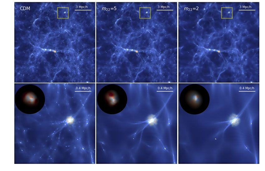
time. The cutoff scale in the matter power spectrum compared to We start by showing a series of maps illustrating images of
CDM can be characterised by the value of k J at the epoch ofmatter- different scales of the intergalactic medium (IGM) in Fig. 3. The
radiation equality kJ,eq = 9m22 Mpc−1 . Since k J grows with time,
1/2
images show the simulated gas density field at z = 6 for CDM (left
a small scale mode which was originally oscillating will eventually column panels) in two of the FDM models with bosonic mass of
start to grow. Thus we can see a decaying oscillating feature in FDM m22 = 5 and m22 = 2 (middle and right column panels respectively).
power spectrum for k & kJ,eq . We show maps for the entire simulation volume (upper panels)
Our FDM simulations employ the initial power spectrum at and also a subregion of the volume (lower panels) that hosts a
z = 99 generated by AxionCAMB (Hlozek et al. 2015). Fig. 2 shows star-forming galaxy with stellar mass ∼ 109 M (marked by the
the linear matter power spectra of the FDM models considered in rectangular boxes in the upper panels with side length of 2 Mpc/h).
this study at z = 0, with the CDM power spectrum plotted in The stellar densities of the galaxy are shown in the circular insets.
the black dotted line. For m22 = 2, 5, 10, the corresponding kJ,eq The gas density field is colored by temperature, with scales shown
is equal to 18, 28, 40 Mpc−1 h respectively, consistent with the by the 2D color bar in Fig. 3. The upper panels illustrate that while
suppression scale seen on the corresponding linear power spectrum. the large-scale structures (e.g., filaments, nodes, voids... etc) of
In the upper x axis of Fig. 2, we also show the typical halo mass the gas distribution stay virtually the same between the runs with
for a particular matter power spectrum wavenumber. This allows different DM physics, the small-scale structures are smeared out
us to get a better idea of what halo mass range the different FDM in the FDM models. The smaller the bosonic DM mass is, the
cutoffs scales affect. We convert the wavenumber to the halo virial more severe the small-scale structures have been washed out. This
mass using Mh = 4π(π/k)3 ρm /3, where ρm = 3H02 Ωm /8πG is the becomes particularly evident in the lower sub-panels where we zoom
background matter density of the universe. into the environment around one small halo. Around this particular
We note that, in comparison with WDM models, the suppres- halo, the gas density is more concentrated and the colors show that
sion in the FDM models with e.g. m22 = 5 is similar to that of the gas has been heated more in the CDM model compared to its
a WDM candidate of sterile neutrino with mν ∼ 1.6 keV through FDM counterparts. As discussed in previous works, this is due to
MNRAS 000, 1–15 (2019)Hydrodynamic simulations of Fuzzy Dark Matter using MP-Gadget 5
5.5
5
log10 (T[k])
4.5
4
0.2 1 5
/ ave
Figure 3. Upper panels : Large-scale gas density field at z = 6 in the simulations of CDM (left panels) and FDM models with m22 = 5 (center) and m22 =2
(right). Bottom panels : The zoomed-in regions of 2 Mpc/h on the side (marked by the rectangular areas in the upper panels) to better illustrate the small-scale
structures, in particular how they are smeared out in the FDM scenarios. The gas density field is color-coded by temperature (blue to red indicating cold to hot
respectively, see the 2D color bar aside). The circular inserts in the bottom panels show the zoomed-in stellar density of the galaxy at the center of the panels.
It is color-coded by the age of the stars (from blue to red, indicating young to old populations respectively). The radius of the zoomed-in circular region is 40
kpc/h and the mass of the galaxy is about 7 × 10⁸ M . Rightmost panel: The 2D color bar shows the values of the gas density and associated temperature. The
temperature and density range are the same for all six panels. Here ρave represents the average surface density shown in the volume.
density of the zoom-in regions with radius 40 kpc/h centered on
the galaxy, colored by the age of stars with blue to red indicating
200 CDM young to old. In the FDM scenario, the galaxy is systematically
m22 = 2 younger than its CDM counterpart. The average age of stars in the
m22 = 5 galaxy is 114, 108 and 88 Myrs for CDM and FDM m22 = 5, 2
150 m22 = 10 scenarios respectively. Generally, the galaxy formation process at
stellar age [Myr]
high redshift is found to be delayed in DM models with primordial
power spectrum cutoff features (e.g. for WDM, see Bode et al. 2001).
To illustrate this further in our simulations, in Fig. 4 we show the
100 average, global stellar age in the whole volume as a function of
redshift. The global stellar age in the FDM models is smaller than
the CDM prediction for a given redshift, and the discrepancies get
50 smaller with decreasing redshift. This is another illustration of why
one should look at high redshift to see prominent effects of FDM
10 9 8 7 6 5 models on the galaxy population.
z
Figure 4. The globally average stellar age in CDM and the three FDM models 3.1 Impacts of FDM on the Halo Mass Functions
as a function of redshift. The star formation process is systematically delayed To compare with previous work which employed N-body simula-
in the FDM models compared to their CDM counterpart.
tions of FDM, we start by showing the halo mass functions (MFs)
for the four different DM models in the redshift range of z = 6 − 9
in Fig. 5. The black lines show the CDM predictions whilst lines
the fact that in FDM models, the volume occupied by the halos is in purple, blue, and red are for FDM models with m22 = 10, 5, 2
systematically larger as a consequence of the delayed dynamical respectively. The dotted lines are the original MFs constructed from
collapse of the halo (see, e.g., Nori et al. 2019). Finally, in the the entire halo catalog. Dash-dotted lines are the expected halo MF
circular insets in the lower panels of Fig. 3, we show the stellar after the removal of spurious halos according to the analytic fitting
MNRAS 000, 1–15 (2019)6 Y. Ni et al.
1 formula provided by Schive et al. (2016), as we will discuss later.
z=9.00 CDM z=8.00
m22 = 2 Solid lines are the halo MFs of luminous halos, and the shaded areas
Mh /[dex 1Mpc 3])
0 m22 = 5 show their Poisson error bars.
m22 = 10
1 As expected from the input matter power spectra shown in
Fig. 2, the halo MF is suppressed in FDM models compared to CDM.
2
Take z = 6 as an example, FDM halo abundance is suppressed
by & 50% for halos in mass range Mh . 1010 M for m22 = 2
log10(
3
(. 5 × 10¹⁰ M for m22 = 10). The suppression gets larger for
4 smaller values of m22 and becomes more prominent as redshift
1
z=7.00 z=6.00 increases. From the dotted lines in Fig. 5, we can see that at mass
Mh /[dex 1Mpc 3])
0 scales close to Mh ∼ 109 M , an upturn feature in the halo MF,
which is especially prominent for m22 ≤ 5, is exhibited in FDM
1
model results. This is likely due to a numerical artifact. Similar to
2 WDM models that predict this small-scale structure suppression,
it is known that FDM simulations also suffer from the problem of
log10(
3 artificial fragmentation of filaments and contains spurious small
halos (see, e.g. Wang & White 2007; Lovell et al. 2014, for WDM
4
9 10 11 9 10 11 studies of spurious halos). Several techniques have been proposed
log10[Mh/M ] log10[Mh/M ] (as we will discuss later in this section) to detect and remove spurious
halos for improving estimations of the true halo MF, upon which
Figure 5. Halo MF of CDM and FDM models for z = 6 − 9. Dotted lines
are the original MFs constructed using the entire halo catalog. Solid lines they can be used to infer the UV LF and compare with observations.
represent the MFs of luminous halos, which are defined as halos that host However, we argue in the rest of this section that spurious halos have
galaxies with M∗ > 5 × 10⁶ M . The shaded areas show the Poisson error negligible effects on galaxy population because the luminous halos
bars. Dash-dotted lines are the analytic halo MF fitting formula from Schive that host galaxies are more massive than the halo mass range where
et al. (2016) (with spurious halos removed) for each FDM models. this numerical artifact becomes important.
To quantify the halo mass range for spurious fragmentation,
Sphericity distribution at z=6 Sphericity of luminous halo Wang & White (2007) provides an empirical estimation, Mlim =
CDM 10.1 ρ̄d/kpeak
2 , of which below this halo mass scale M
lim halos are
0.8 m22=10 dominated by numerical artifacts rather than physical ones. Here ρ̄
is the mean density of the universe, kpeak is the wavenumber at the
0.6
maximum of the dimensionless matter power spectrum, and d is the
mean interparticle separation. In our FDM model with m22 = 2,
S
0.4
Mlim ∼ 2 × 10⁹ M (for m22 = 10, Mlim ∼ 4 × 10⁸ M ) corresponds
0.2 to the upturn feature in our original halo MFs.
M * > 5 × 10⁶M Other than simply applying a mass cut corresponding to Mlim ,
0.0 additional discriminating criteria have been developed to refine the
CDM
0.8 m22=2
removal of those artifacts. One common method is to trace the La-
grangian region occupied by the halo member particles back to the
0.6 simulation initial condition (protohalo) and use their spatial distri-
butions (e.g., shape) as a proxy to discern the spurious ones. Another
S
0.4 method is to match halos between different resolution runs for which
a spurious halo would not be present in the higher resolution runs
0.2
M * > 5 × 10⁶M (see, e.g. Schive et al. 2016, for the discussions in the FDM scenar-
ios). Schive et al. (2016) has provided an analytic fitting function
0.0
9 10 11 9 10 11 for which we can derive the expected spurious-halo-free MF for
log10[Mh/M ] log10[Mh/M ] a given FDM model. However, we note that this does not predict
whether a halo is spurious or not, but rather shows the expected
Figure 6. The comparison of halo sphericity distributions in CDM with
FDM halo population for a given halo mass range. In Fig. 5 we
those from two FDM models (top panels: with m22 =10; bottom panels: with
m22 =2) at z = 6. The sphericity is calculated based on DM component only.
show the "corrected-halo MF" as dash-dotted lines with spurious
The left panels show the distributions of all the halos in the two simulations, halos removed. Comparing this corrected-MF with MF of luminous
with grey contours representing CDM and colored contours for FDM models halos (solid lines), we can see that the luminous halo population in-
(blue: m22 = 10; red : m22 = 2). The right panels show the population of deed doesn’t extend to the halo mass region where the corrected-MF
luminous halos, with the same color scheme as the left panels. Solid lines (dash-dotted lines) starts to deviate from original MF (dotted lines).
in all panels, which have the same color scheme as the contours, give the Therefore it suggests that it is not necessary to apply spurious halo
average sphericity of halos in the corresponding mass bins. removal if we are concerned with deriving quantities from luminous
galaxies in our simulations.
As a further illustration, we also calculate the haloq sphericity S
I1 +I2 −I3
in the same way as defined in Schive et al. (2016): S = −I 1 +I2 +I3
,
with I1 6 I2 6 I3 the principle moments of inertia of the halos.
Note S is calculated merely based on DM component. In Fig. 6 we
show S in CDM and two FDM models with m22 = 10 (top panel)
MNRAS 000, 1–15 (2019)Hydrodynamic simulations of Fuzzy Dark Matter using MP-Gadget 7
and m22 = 2 (bottom panel) for halos identified at z = 6. It has 1.0
(nF, lum/nF, tot)/(nC, lum/nC, tot)
been shown in previous studies that genuine halos are those with
high S (close to 1) while spurious halos occupy low S regions. For 0.8
example, Schive et al. (2016) suggests a cut of S>0.3 for removing
spurious halos in the redshift range of z = 4 − 10. The solid lines 0.6
in Fig. 6, which show the average S of each model as a function
of halo mass Mh , indicate that discrepancies of S between CDM 0.4
and FDM models are the most prominent at Mh . 5 × 10⁹ M m22 = 2
for m22 = 2 and Mh . 109 M for m22 = 10. This is consistent 0.2 m22 = 5
m22 = 10
with the Mlim we derived before. However, in the right panels of
Fig. 6 where we only select the luminous haloes (which will have
0.0
the actual contribution to the calculated LFs), the distributions of 0.0
S of all DM models occupy the similar high S regions with only
MFDM MCDM
a few exceptions. All these results indicate that the luminous halos
in our simulation are highly unlikely to be spurious halos. This is
0.5
1.0
due to the fact that very low mass halos do not have deep potentials
to maintain enough gas to have efficient star formation. Therefore
most of the low mass halos, including those generated by numerical
M * > 5 × 10⁶M
artifacts, do not host galaxies. We hence conclude that the process 1.5
of removing spurious halos is not required in our study of the high-z
2.0
1.0
galaxy population for which the effects remain negligible.
3.2 Galaxy Stellar Mass Function
0.8
AFDM/ACDM
Before we discuss the results for the GSMFs, we compare the popu-
lation of luminous galaxies in CDM and FDM models as a function
of halo mass. In the top panel of Fig. 7, we show the ratio of the 0.6
luminous fraction of halos hosting galaxies in FDM compared to
CDM models as a function of halo mass. We define the luminous 0.4
fraction, nlum /ntot , as the fraction of halos that host at least one
galaxy with M∗ > 5 × 10⁶ M . The plot shows that below the halo
mass, Mh . 1010 M , at which the FDM halo mass function starts to 9.5 10.0 10.5 11.0
deviate from the CDM one the luminous fraction in FDM becomes log10[Mh/M ]
significantly smaller (. 70%) than in CDM. More specifically, for
example, in the FDM model with m22 = 2 the luminous fraction is Figure 7. Top panel: The ratio of the fraction of halos hosting luminous
suppressed by ∼ 80% for halos with Mh ∼ 1010 M at z = 6. This galaxies in FDM versus those in CDM as a function of halo mass (with
M∗ ≥ 5 × 10⁶ M ). Middle panel: The difference in the UV band magnitude
indicates that the suppression on galaxy number density is caused
between FDM and CDM galaxies as function of halo mass. Lower panel:
not only by the decreased halo number density (ntot ) in the FDM
The ratio of average stellar age in galaxies between CDM and FDM models
scenario but also by the fact that FDM halos are less likely to host as a function of halo mass. For all the three panels, solid lines show results
galaxies compared to their CDM counterparts. at z = 6, and the dotted lines are from z = 8.
In the middle panel of Fig. 7, we show the difference in the UV
magnitude for the galaxies (based on the stellar population synthesis
model described in Section 2.1) in the FDM and CDM models as galaxy UV magnitudes between CDM and FDM (shown in the
a function of halo mass. We find that for galaxies hosted by halos middle panel of Fig. 7).
with Mh ∼ 1010 M , the average UV band luminosity at z = 6 in Although the halo mass is a direct indicator of the underlying
FDM model with m22 = 2 is about 0.5 mag smaller (brighter) than density fluctuation scale, it is not directly measured (at least in
that in CDM. Thus, we conclude that although haloes in the FDM any of the high-redshift observations discussed in this work). Next,
model with Mh . 1010 M are less likely to host luminous galaxies we examine the direct predictions for the galaxy abundances as a
compared to the ones in CDM; the galaxies that do emerge in FDM function of stellar mass. In particular, in Fig. 8 we show the GSMFs
models are typically somewhat brighter than those in CDM. for CDM and FDM models in the redshift range of z = 5 − 10.
The reason galaxies in FDM models tend to be more luminous For comparison, the black dotted lines show the GSMFs in the
than in CDM is likely due to the delayed star formation process in BlueTides simulation, (which has only been run to z = 7). The
the former as this leads to a younger and brighter stellar population. shaded areas represent 1σ error from expected cosmic variance in
To directly examine the age of the stars in galaxies, we show the a volume of 15 Mpc/h side length. Note that our smaller volume
ratio of average stellar ages of galaxies between FDM and CDM as a realization of CDM tends to be slightly lower than the one from
function of halo mass (in the lower panel of Fig. 7). The galaxies in the BlueTides, which is derived from a large simulation volume
FDM models are indeed generally younger than those in CDM, an of 400 Mpc/h side length. However, our results are well within the
effect that becomes even more prominent as the halo mass decreases. expected cosmic variance.
For example, galaxies that reside in halos with Mh ∼ 1010 M for Fig. 8 shows that there is a suppression on galaxy abundance
FDM with m22 = 2 at z = 6 have average age about 40% of their in FDM compared to CDM, and the suppression increases with de-
CDM counterparts, while for Mh ∼ 3 × 10¹⁰ M (log10 Mh = 10.5) creasing stellar mass. For example, at z = 6 the galaxy abundance is
the ratio is about 60%. This directly explains the difference in the suppressed by & 50% for stellar masses M∗ . 107 M (. 108 M )
MNRAS 000, 1–15 (2019)8 Y. Ni et al.
0.5
BlueTides CDM BlueTides
z=10 z=9 z=8
M * /[dex 1Mpc 3])
1.0 m22 = 2 Song2016
m22 = 5
1.5 m22 = 10
BlueTides
2.0
2.5
3.0
log10(
3.5
4.0
0.5
BlueTides Stefanon2017 Stefanon2017
z=7 z=6 z=5
M * /[dex 1Mpc 3])
1.0 Grazian2015 Grazian2015 Grazian2015
Gonzalez2011 Gonzalez2011 Gonzalez2011
1.5 Duncan2014 Duncan2014 Duncan2014
Song2016 Song2016 Song2016
2.0
2.5
3.0
log10(
3.5
4.0
7 8 9 10 7 8 9 10 7 8 9 10
log10[M * /M ] log10[M * /M ] log10[M * /M ]
Figure 8. The GSMFs predicted in CDM (red lines) and FDM models with m22 = 10, 5 and 2 (purple, green, and blue lines respectively) shown for z = 5 − 10.
The color shaded areas are the 1 σ cosmic variance uncertainties for a comoving volume of 15 Mpc/h per side. This is estimated based on subvolumes drawn
from the BlueTides simulation as described in the text. The green vertical dash-dotted lines mark the limits for JWST deep field Observational data points
with 1 σ error bars include results from González et al. (2011) (orange triangles), Duncan et al. (2014) (pink triangles), Grazian et al. (2015) (grey squares),
Song et al. (2016) (blue circles), and Stefanon et al. (2017) (green triangles).
in the FDM model with m22 = 5 (m22 = 2). To quantify how the probe out to the highest redshift (z = 8) and to the smallest stellar
suppression evolves with redshift, we plot, in the upper panel of masses (M∗ . 107 M ). Their measurements are obtained through
Fig. 9, the ratio of galaxy abundance in FDM over that in CDM the combination of HST imaging data together with the deep IRAC
(different line styles show different stellar mass range) as a function data from Spitzer Space Telescope over the Great Observatories
of redshift. This shows that the suppression of the galaxy abundance Origins Deep Survey (GOODS) fields and the HUDF. In Fig. 8 we
brought in by FDM decreases for decreasing redshift. For example, can see that, at z = 5 − 8, both our predictions for φM∗ in the CDM
the abundance of galaxies (from GSMF) with stellar mass range of and FDM model with m22 = 10, 5 are consistent with the Song et al.
1 − 3 × 10⁷ M (solid lines) is suppressed by ∼ 40% in the FDM (2016) data, while the m22 = 2 model appears inconsistent for stel-
model m22 = 5 (in blue) at z = 9 , while this suppression is reduced lar masses below M∗ . 108 M . Note that, although the González
to ∼ 20% at z = 5. et al. (2011) data agrees with our m22 = 2, it is systematically lower
Next, we compare the predictions for GSMFs from FDM mod- than the rest of the observational data sets. Therefore we do not take
els with the current observational constraints. Observational mea- it into consider when we derive our FDM limits.
surements of the GSMF are typically obtained by taking the ob- We now wish to quantify more precisely the level of discrep-
served rest-frame UV LFs and convolving them with a stellar mass ancy between the model and observational measurements. To do so
versus UV luminosity distribution at each redshift. The advantage we adopt a procedure similar to Menci et al. (2017). In particular,
of using GSMFs is that GSMFs can be easily derived from our we calculate the expected cumulative number density nobs from data
hydrodynamic simulations, once run, without any further assump- within the stellar mass range of M∗ = 107 − 109 M and compare
tions. In Fig. 8 we show the current available observational data it with the abundance predicted from the simulations for each DM
on GSMFs (φM∗ ) collected from González et al. (2011) (orange model. To quantify the observational uncertainties, we rebuild 107
triangles), Duncan et al. (2014) (pink triangles), Grazian et al. realizations of galaxy stellar mass distributions by taking random
(2015) (grey squares), Song et al. (2016) (blue circles), Stefanon value φM∗ in each mass bin according to a log-normal distribution
et al. (2017) (green triangles). Among these studies, Song et al. with the variance given by the corresponding error bars. Then we
(2016) provides the strongest constraints on φM∗ for FDM as they calculate the cumulative number density nobs for each realization
MNRAS 000, 1–15 (2019)Hydrodynamic simulations of Fuzzy Dark Matter using MP-Gadget 9
1.0 1.2
0.8 1.4
GSMF
log10(nM * /[Mpc 3])
1.6
nFDM/nCDM
0.6
1.8
0.4 2.0 Song2016
median
m22 = 2 2.2 1
0.2 z=5 2 z=6
m22 = 5 2.4 3
0.0 m22 = 10 2 4 6 8 10 CDM 2 4 6 8 10 CDM
m22 m22
1.0 Figure 10. The cumulative number density of galaxies with mass 107 M <
M∗ < 109 M at z = 5 (left panel) and z = 6 (right panel) as function
0.8
UVLF
of m22 . The CDM results are marked by the rightmost orange points. We
nFDM/nCDM
add 1σ cosmic variance on simulation data points based on volume of
0.6 (15Mpc/h)3 and (24Mpc/h)3 (comparable to the HFF and HUDF effective
volumes). The cosmic variance is estimated from the BlueTides simulation.
0.4 The horizontal lines represent the observed galaxy number densities within a
given mass bin with 1σ (dash lines), 2σ (dotted lines), and 3σ (dash-dotted
0.2 lines) confidence levels. The observational data set used here is from Song
et al. (2016).
0.0
5 6 7 8 9 10
z extending to small mass or with larger volumes may thus be needed
to put further constraints on FDM models with m22 & 5 from
Figure 9. Upper panel: The ratio of the luminous halo fraction in three the GSMF. In Fig. 8, we show the expected detection limit for
FDM models versus CDM as function of redshift, which is derived from the JWST deep field with survey volume comparable to HUDF in the
GSMFs at two different stellar mass bins: [107 M ,3 × 107 M ] (solid lines), vertical green dash-dotted lines. This is expected to probe to M∗ .
[5 × 10⁶ ,107 M ] (dotted lines). Lower panel: The same as the upper panel, 107 M . The detection limit estimated for JWST lensed field with
but with UV LFs over two magnitude bands of [-14.5, -16] (solid lines) and 10× magnification can further extend down to M∗ ∼ 106 M (Yung
[-13,-14.5] (dotted lines).
et al. 2019a). To roughly estimate how JWST can put constraints at
this stellar mass region, we use galaxies below our mass threshold
of galaxy (M∗ > 5 × 10⁶ M ) and calculate the galaxy abundance
and derive the median and the uncertainties in nobs from the con-
around M∗ = 106 M with cosmic variance estimated based on
structed distribution (out of the 107 nobs realizations). In Fig. 10
volume of (24Mpc/h)3 . We speculate that JWST should be able to
we compare the nobs derived from Song et al. (2016) with our sim-
distinguish FDM models m22 & 5 with CDM by measuring the
ulation results at z = 5 and z = 6. We choose these two redshifts
GSMFs down to masses ∼ 106 M where the difference in galaxy
because the observational data set has smaller error bars and thus
population from different DM models becomes more significant.
should provide the most competitive constraint for FDM models.
Although the GSMF is straightforward to predict from hydro-
The horizontal lines show the median (the solid lines) and 1σ, 2σ,
dynamical simulations, the galaxy LFs are the direct observable.
3σ lower bounds (the dashed, the dotted, and the dash-dotted lines
Also, recent measurements of UV LF have extended further into
respectively) of nobs derived from the observations. The data points
the faint end of the galaxy population using lensed fields, which is
marked with the red cross give the cumulative number density, n M∗ ,
important for constraining the FDM model. Therefore, in the next
obtained from our simulations for the different FDM models, while
section, we examine our model predictions in a converse way: we
the CDM predictions are shown by the orange points (on the right).
derive UV magnitude of galaxies from the simulations and directly
By comparing the lower bounds of nobs with our predicted n M∗ ,
compare with the observed LFs.
we infer that the FDM model with m22 < 2 is ruled out at the 3σ
confidence level by this data set. If we interpolate our models, we
obtain that m22 . 4 can be ruled out by 2σ confidence level at
3.3 Galaxy Luminosity Function
z = 6, although the constraint is slightly weaker at z = 5.
The galaxies with inferred mass log(M∗ /M ) < 8.5 (z = 5−8) During the last decades, rapid progress has been made and increas-
primarily come from the HUDF observations (a 2.4’ × 2.4’ field) ing numbers of high−z faint galaxies have been discovered. Much
(Song et al. 2016). In Fig. 10 we also add the cosmic variance of this progress has come with the installations of new instruments,
on n M∗ for volume of (24Mpc/h)3 which is comparable to HUDF such as HST/WFC3 (Windhorst et al. 2011), and the many associ-
survey volume. As described in Section 2.1, the expected cosmic ated extremely deep surveys that have been carried out, e.g. Cosmic
variance is calculated directly from the galaxy population in the Assembly Near-IR Deep Extragalactic Legacy Survey (CANDELS;
large volume BlueTides simulation. Taking this into account, we Grogin et al. 2011), GOODS (Giavalisco et al. 2004), HUDF (Beck-
infer that the predicted n M∗ from the m22 = 5 model is within with et al. 2006), the Cluster Lensing And Supernova survey with
the 1σ of the cosmic variance for the CDM model at both z = 5 Hubble (CLASH; Postman et al. 2012), the Early Release Science
and z = 6, indicating that in the mass band M∗ = 107 − 109 M , field (ERS; Windhorst et al. 2011), and the Brightest of Reionizing
a survey of HUDF volume will not be able to distinguish clearly Galaxies Survey (BoRG; Trenti et al. 2011). Also, applying tech-
between m22 = 5 and CDM (within cosmic variance). Surveys niques such as lensing magnification through galaxy clusters have
MNRAS 000, 1–15 (2019)10 Y. Ni et al.
BLUETIDES CDM BLUETIDES
0 z=10 Bouwens2015 z=9 m22 = 2 z=8 Bouwens2015
Bouwens2015_ulimit m22 = 5 Bouwens2015_ulimit
log10[ /Mpc 3mag 1]
Bouwens2016 m22 = 10 Atek2015
1 BLUETIDES Finkelstein
Ishigaki
J×10 J H Bouwens2016
Ishigaki Laporte
Livermore
Laporte
2
3
4
5
BLUETIDES Bouwens2015 Bouwens2015
0 z=7 Bouwens2015 z=6 Atek2018 z=5
Bouwens2015_ulimit Finkelstein
log10[ /Mpc 3mag 1]
Atek2015 Livermore
1 Finkelstein
Ishigaki
Bouwen17
Laporte
Livermore
2
3
4
5
14 16 18 20 22 14 16 18 20 22 14 16 18 20 22
MUV MUV MUV
Figure 11. LFs for CDM (black solid lines) and FDM models with m22 = 10 (purple lines), 5 (blue lines), and 2 (red lines) at redshift z = 5 − 10. The colored
shaded areas are 1σ error cosmic variance for a volume of 15 Mpc/h side length estimated based on BlueTides simulation results. The black dotted lines are
the results of the BlueTides simulations. The blue vertical dashed line is the detection limit for HUDF. Green vertical dash-dotted lines represent the detection
limit expected for a JWST deep-field with survey volume comparable to the HUDF. Red vertical dotted lines represent the expected MUV limit for JWST
lensed fields with 10 × magnification. (The apparent magnitudes of the three lines are mAB,lim = 30.0, 31.5, and 34 respectively). For z = 6 − 9, the data (at
MUV ≥ −17) is from the analysis of HFF program applying the gravitational lensing techniques (Atek et al. 2015, 2018; Livermore et al. 2017; Ishigaki et al.
2018). We use Livermore’s Eddington-corrected data points shown in Yung et al. (2019b).
yielded intriguing results for the faint-end LF observations. In par- binned in mass), the suppression of faint-end LFs decreases with
ticular, the HFF program has been able to identify sources that are decreasing redshift. For example, in the FDM model with m22 = 5
intrinsically fainter than the limits of the current unlensed surveys, (in blue) model, the abundance of galaxies within magnitude range
extending the observed UV LFs to MUV ∼ -13 − -15 (Atek et al. of −16 < MUV < −14 is suppressed by . 60% at z = 9 compared
2015; Livermore et al. 2017; Ishigaki et al. 2018). to CDM, but the suppression is only . 20% at z = 5.
Fig. 11 shows the LFs of CDM (black lines) and the three FDM In Fig. 12, we compare the LFs from our simulations to those
models (with purple, blue, and red solid lines for FDM with m22 from Schive et al. (2016), which were derived by applying a con-
= 10, 5, and 2 respectively) at z = 5 − 10. Shaded areas represent ditional LF model on DM halo mass function constructed from
the expected 1σ cosmic variance uncertainties of comoving volume cosmological simulations (DM-only). In particular, they employed
with 15 Mpc/h side length for each DM model. Black dotted lines the least χ-square fitting on the observational data by Bouwens et al.
with black triangle points show the results from the BlueTides (2015) to determine the best-fit parameters for each conditional LF
simulations for comparison. We can see that there is a marked model applied to the different DM scenarios. In Fig. 12 we show
suppression of faint-end LFs in the FDM models and the suppression their predicted LFs for CDM and FDM with m22 = 1.6 (with black
becomes more prominent for decreasing values of the FDM boson and orange dash-dotted lines) and compare these with the LFs gen-
mass, m22 . If we take z = 6 as an example, the galaxy abundance erated by our direct hydrodynamical simulations (black and red
is suppressed by > 50% for MUV & −15 (MUV & −17) for FDM solid lines respectively). Our predictions of LFs, either for CDM
m22 = 5 (m22 = 2) model. To trace the time evolution of the or FDM, are somewhat systematically lower than the Schive et al.
suppression, we show (in the lower panel of Fig. 9) the ratio (at (2016) models. Nevertheless, in the lower panel of Fig. 12, where
the faint-end) of the galaxy number density between CDM and we show the comparison of the ratio of FDM over CDM number
FDM models (in different UV magnitude bin) as a function of density in both studies, we can see that the amount the suppression
redshift. Similar to the effects on the GSMF (galaxy number density as a function of magnitude is in good agreement with each other
MNRAS 000, 1–15 (2019)Hydrodynamic simulations of Fuzzy Dark Matter using MP-Gadget 11
3.3.1 Comparison with observations
0 The observational data shown in Fig. 11 have been collected
z=8 CDM from multiple studies. For a brief summary here, Bouwens et al.
m22 = 1.6 (2015) utilizes data sets from CANDELS, HUDF, ERS, and the
log10[ /Mpc 3mag 1]
1 Schive CDM BoRG/HIPPIES programs, and Finkelstein et al. (2015) uses data
Schive m22 = 1.6 sets from CANDELS/GOODS, HUDF, the HFF parallel fields near
2 cluster MACS J0416.1-2403 and Abell 2744. Livermore et al.
(2017) combines HFF data of the Abell 2744 and MACS J0416.1-
2403 clusters, and in this paper we refer to the Eddington corrected
3
version of the Livermore et al. (2017) data shown in Yung et al.
(2019b). Laporte et al. (2016) combines Hubble and Spitzer data
4 from MACS J0717.5+3745 cluster and its parallel field. Bouwens
-70 et al. (2017) uses galaxy samples from four most massive clusters
in HFF to provide prediction for LF at z ∼ 6 while Atek et al.
1)%
-80 (2018) combines data sets of all 7 clusters from the HFF program.
In Ishigaki et al. (2018) they utilize the complete HFF data. For
Schive m22 = 1.6
C
-90 the constraints on the faintest populations (MUV ≥ −17), where the
( F/
m22 = 1.6 discrepancies between different DM models become distinctive, all
-100
13 14 15 16 17 18 19 of the observational data sets available now (e.g., Atek et al. 2015,
MUV 2018; Livermore et al. 2017; Ishigaki et al. 2018) are obtained by tak-
ing advantage of lensing magnification by the massive foreground
galaxy clusters. This technique has the great potential to probe fur-
Figure 12. The comparison between our predicted LFs and those from ther into the faint-end LFs, however, it also suffers from significant
Schive et al. (2016) at z = 8. Upper panel: Black and orange dash-dotted
systematics (e.g., see discussions in Menci et al. 2017). As shown in
lines are the Schive et al. (2016) results for CDM and FDM with m22 = 1.6
Fig. 11, there are sometimes some discrepancies between different
respectively. They are obtained by applying conditional LF model on their
halo mass function. Black and red solid lines are the predictions from observations at several redshifts (e.g., MUV & −15 at z = 6) in the
our hydrodynamical simulation with the same FDM bosonic mass. The faint-end of the measured LFs (even though all measurements agree
color-shaded areas are the estimated 1σ cosmic variance on volume of with each other within 1 σ due to large observational uncertainties).
(15Mpc/h)3 . Lower panel: The ratio of FDM LFs over their CDM counter- Bouwens et al. (2017) shows that for highly-magnified sources the
parts from this work and the Schive et al. (2016) results. systematic uncertainties can imply up to orders of magnitudes dif-
ferences. Therefore the current constraints in range of MUV & −15
at z > 4 are still under significant debate.
0.5 Despite the large uncertainties, the LF data from the lensed
fields can extend to fainter MUV thresholds than those from the
unlensed data, such as those used by Song et al. (2016) to infer
1.0
log10(nMUV/[Mpc 3])
the GSMFs. Therefore we expect that some of the LF observa-
tions (especially those which adopted the lensed samples to reach
1.5 MUV & −17) can place important constraints on FDM models.
Atek18 Livermore Using a similar procedure described in the previous section, we
2.0 median median compare the cumulative galaxy number density over certain mag-
1 1
z=6 2 z=7 2 nitude band nobs derived from observations with our DM model
3 3 predictions (shown in Fig. 13) at z = 6 and z = 7. Although the
2.5
2 4 6 8 10 CDM 2 4 6 8 10 CDM discrepancies between FDM and CDM model predictions increases
m22 m22 with higher redshift, the constraint on FDM does not improve signif-
Figure 13. Cumulative number densities of galaxies for −18 6 MUV 6 −14 icantly by using data sets from z > 7 due to the large observational
at z = 6 (left panel) and at z = 7 (right panel) as function of m22 . The uncertainties at higher redshifts (and/or complete lack of data other-
error bars correspond to the 1σ cosmic variance of effective volume of wise). So we will restrict our analysis to z = 6, 7 and calculate nobs
(15Mpc/h)3 (grey or orange error bars) and (24Mpc/h)3 (light grey error using the magnitude range of −18 6 MUV 6 −14. At z = 6 we do
bars) both calculated from BlueTides. The horizontal lines represent the not extend down to MUV > −14 again due to the large uncertainties
observed cumulative galaxy number density within the same magnitude in the observational data sets.
band with 1σ (dash lines), 2σ (dotted lines), and 3σ (dash-dotted lines)
confidence levels. The data set used is from Atek et al. (2018) for z = 6 and For the purpose of this analysis, we choose the data sets that
Livermore et al. (2017) with Eddington correction for z = 7. are the most consistent with our CDM prediction as those allow
us to quantify the constraints on FDM models more reliably. In
Fig. 13, the horizontal lines indicate the median (the solid lines),
within 5%. Therefore both models have captured similar effects of 1σ, 2σ, and 3σ lower bounds (the dash, the dotted, and the dash-
FDM with regards to suppressing the galaxy LFs. In essence, the dotted lines) of nobs obtained from Atek et al. (2018) at z = 6 (left
results from full hydrodynamical simulations of galaxy formation panel) and Livermore et al. (2017) (Eddington-corrected version
predict LFs that do not differ systematically from the Schive et al. from Yung et al. (2019b)) at z = 7 (right panel). The data points
(2016) predictions. This is a promising result, implying that the LF marked by the red cross are cumulative number densities (nMUV )
predictions from FDM are somewhat stable against different galaxy obtained from different FDM simulations, while CDM models are
formation models. indicated by the rightmost points. Comparing the predicted nMUV
MNRAS 000, 1–15 (2019)You can also read