Angular Visual Hardness - ICML Proceedings
←
→
Page content transcription
If your browser does not render page correctly, please read the page content below
Angular Visual Hardness
Beidi Chen 1 Weiyang Liu 2 Zhiding Yu 3 Jan Kautz 3 Anshumali Shrivastava 1
Animesh Garg 3 4 5 Anima Anandkumar 3 6
Abstract
Recent convolutional neural networks (CNNs)
have led to impressive performance but often suf-
fer from poor calibration. They tend to be over-
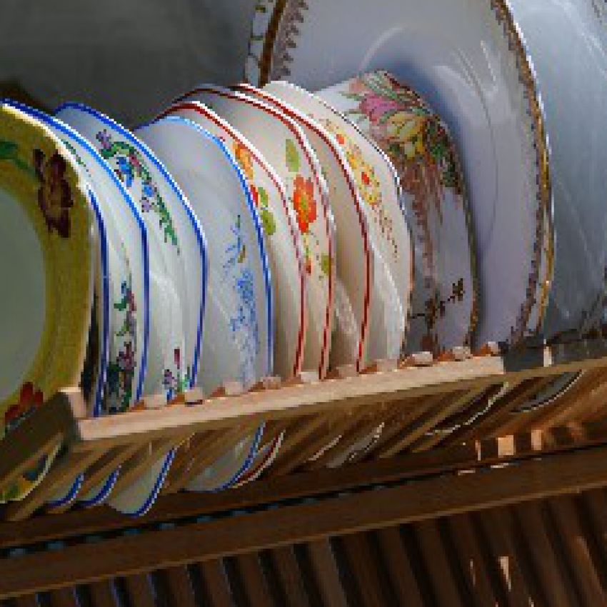
Plate Rack Sharpness Contrast Blur
confident, with the model confidence not always
reflecting the underlying true ambiguity and hard-
ness. In this paper, we propose angular visual
hardness (AVH), a score given by the normalized
angular distance between the sample feature em-
Dishwasher Saltshaker Nail Oil Filter
bedding and the target classifier to measure sam-
ple hardness. We validate this score with an in- Figure 1. Example images that confuse humans. Top row: images
with degradation. Bottom row: images with semantic ambiguity.
depth and extensive scientific study, and observe
that CNN models with the highest accuracy also
have the best AVH scores. This agrees with an have even surpassed human-level performance (Deng et al.,
earlier finding that state-of-art models improve on 2009). Despite the notable progress, CNNs are still far
the classification of harder examples. We observe from matching human-level visual recognition in terms of
that the training dynamics of AVH is vastly dif- robustness (Goodfellow et al., 2014; Wang et al., 2018c),
ferent compared to the training loss. Specifically, adaptability (Finn et al., 2017) and few-shot generalizabil-
AVH quickly reaches a plateau for all samples ity (Hariharan & Girshick, 2017; Liu et al., 2019), and could
even though the training loss keeps improving. suffer from various biases. For example, ImageNet-trained
This suggests the need for designing better loss CNNs are reported to be biased towards textures, and these
functions that can target harder examples more ef- biases may result in CNNs being overconfident, or prone to
fectively. We also find that AVH has a statistically domain gaps and adversarial attacks (Geirhos et al., 2019).
significant correlation with human visual hard- Softmax score has been widely used as a confidence measure
ness. Finally, we demonstrate the benefit of AVH for CNNs but it tends to give over-confident output (Guo
to a variety of applications such as self-training et al., 2017; Li & Hoiem, 2018). To fix this issue, one line
for domain adaptation and domain generalization. of work considers confidence calibration from a Bayesian
point of view (Springenberg et al., 2016; Lakshminarayanan
et al., 2017). Most of these methods tend to focus on the cal-
1. Introduction
ibration and rescaling of model confidence by matching ex-
Convolutional neural networks (CNNs) have achieved great pected error or ensemble. But how much they are correlated
progress on many computer vision tasks such as image clas- with human confidence is yet to be thoroughly studied. On
sification (He et al., 2016; Krizhevsky et al., 2012), face the other hand, several recent works (Liu et al., 2016; 2017c;
recognition (Sun et al., 2014; Liu et al., 2017b; 2018a), and 2018b) conjecture that softmax feature embeddings tend to
scene understanding (Zhou et al., 2014; Long et al., 2015a). naturally decouple into norms and angular distances that are
On certain large-scale benchmarks such as ImageNet, CNNs related to intra-class confidence and inter-class semantic dif-
1
ference, respectively. While inspiring, their conjecture lacks
Rice University 2 Georgia Institute of Technology 3 NVIDIA thorough investigation and we make surprising observations
4
University of Toronto 5 Vector Institute, Toronto 6 Caltech. Corre-
spondence to: Beidi Chen , Weiyang Liu partially contradicting to the conjecture on intra-class con-
, Zhiding Yu . fidence. This motivates us to conduct rigorous studies for
reliable and semantics-related confidence measure.
Proceedings of the 37 th International Conference on Machine
Learning, Vienna, Austria, PMLR 119, 2020. Copyright 2020 by Human vision is considered much more robust than current
the author(s). CNNs, but this does not mean humans cannot be confused.
Angular Visual Hardness

                                              0                   ing angles, e.g., (Liu et al., 2017b; Deng et al., 2019; Wang
                                              1
                                              2
                                              3
                                                                  et al., 2018b;a). We verify that better models tend to have
              Angle θ(x,wy)
                                              4
                                              5                   better average AVH scores, which validates the argument
                                              6

                        Norm ||x||            7
                                              8
                                                                  in (Recht et al., 2019) that improving on hard examples is
                                              9
                                                                  the key to improved generalization. We show that AVH has
             Classifier wy
                                                                  a statistically significant stronger correlation with human
                                                                  selection frequency than widely used confidence measures
                                                                  such as softmax score and embedding norm across several
                                                                  CNN models. This makes AVH a potential proxy of human
                                                                  perceived hardness when such information is not available.
Figure 2. Visualization of embeddings on MNIST by setting their   Finally, we empirically show the superiority of AVH with its
dimensions to 2 in a CNN.                                         application to self-training for unsupervised domain adap-
Many images appear ambiguous or hard for humans due to            tation and domain generalization. With AVH being an
various image degradation factors such as lighting condi-         improved confidence measure, our proposed self-training
tions, occlusions, visual distortions, etc. or due to semantic    framework renders considerably improved pseudo-label se-
ambiguity in not understanding the label category, as shown       lection and category estimation, leading to state-of-the-art
in Figure 1. It is therefore natural to consider such human       results with significant performance gain over baselines.
ambiguity or visual hardness on images as the gold-standard       Our proposed new loss function based on AVH also shows
for confidence measures. However, explicitly encoding hu-         drastic improvement for the task of domain generalization.
man visual hardness in a supervised manner is generally not
feasible, since hardness scores can be highly subjective and
                                                                  2. Related Work
difficult to obtain. Fortunately, a surrogate for human vi-       Example hardness measures. An automatic detection of
sual hardness was recently made available on the ImageNet         examples that are hard for human vision has numerous ap-
validation set (Recht et al., 2019). This is based on human       plications. (Recht et al., 2019) showed that state-of-the-art
selection frequency (HSF) - the average number of times           models perform better on hard examples. This implies that
an image gets picked by a crowd of annotators from a pool         in order to improve generalization, the models need to im-
belonging to certain specified category. We adopt HSF as a        prove accuracy on hard examples. This can be achieved
surrogate for human visual hardness in this paper to validate     through various learning algorithms such as curriculum
our proposed angular hardness measure in CNNs.                    learning (Bengio et al., 2009) and self-paced learning (Ku-
                                                                  mar et al., 2010) where being able to detect hard examples
Contribution: angular visual hardness (AVH). Given a
                                                                  is crucial. Measuring sample confidence is also important
CNN, we propose a novel score function for measuring sam-
                                                                  in partially-supervised problems such as semi-supervised
ple hardness. It is the normalized angular distance between
                                                                  learning (Zhu; Zhou et al., 2012), unsupervised domain
the image feature embedding and the weights of the target
                                                                  adaptation (Chen et al., 2011) and weakly-supervised learn-
category (See Figure 2 as a toy example). The normalization
                                                                  ing (Tang et al., 2017) due to their under-constrained nature.
takes into account the angular distances to other categories.
                                                                  Sample hardness can also be used to identify implicit distri-
We make observations on the dynamic evolution of AVH              bution imbalance in datasets to ensure fairness and remove
scores during ImageNet training. We find that AVH plateaus        societal biases (Buolamwini & Gebru, 2018).
early in training even though the training (cross-entropy)
                                                                  Angular distance in neural networks. (Zhang et al., 2018)
loss keeps decreasing. This is due to the nature of parameter-
                                                                  uses deep features to quantify the semantic difference be-
ization in softmax loss, of which the minimization goes in
                                                                  tween images, indicating that deep features contain the most
two directions: either by aligning the angles between feature
                                                                  crucial semantic information. It empirically shows that the
embeddings and classifiers or by increasing the norms of
                                                                  angular distance between feature maps in deep neural net-
feature embeddings. We observe two phases popping up dur-
                                                                  works is very consistent with the human in distinguishing
ing training: (1) Phase 1, where the softmax improvement
                                                                  the semantic difference. (Liu et al., 2017c) proposes a hy-
is primarily due to angular alignment, and later, (2) Phase
                                                                  perspherical neural network that constrains the parameters
2, where the improvement is primarily due to significant
                                                                  of neurons on a unit hypersphere and uses angular similarity
increase in feature-embedding norms.
                                                                  to replace the inner product similarity. (Liu et al., 2018b)
The above findings suggest that the AVH can be a robust uni-      proposes to decouple the inner product as norm and angle,
versal measure of hardness since angular scores are mostly        arguing that norms correspond to intra-class variation, and
frozen early in training. In addition, they suggest the need      angles corresponds to inter-class semantic difference. How-
to design better loss functions over softmax loss that can im-    ever, this work does not perform in-depth studies to prove
prove performance on hard examples and focus on optimiz-          this conjecture. Recent research (Liu et al., 2018a; Lin et al.,
Angular Visual Hardness
0.3 0.3 0.3
-0.2 -0.2 -0.2
-0.7 -0.7 -0.7
0.3 0.3 0.3
-0.7 -0.7 -0.7
-0.2 -0.2 -0.2 -0.2 -0.2 -0.2
0.3 0.3 0.3
-0.7 -0.7 -0.7
Figure 3. Visualization of two Gaussian classification. The left plot is input data from two classes (generated Gaussian samples) on the
unit sphere. The middle one is their AVH heatmap, the samples with lighter color are exactly the visually hard examples. Lighter color
represents higher values. The right one is the heatmap for `2 -norm of the feature embeddings, showing no correlation to hard samples.
2020; Liu et al., 2020) comes up with an angle-based hy- Definition 1 (Model Confidence). We define Model Confi-
perspherical energy to characterize the neuron diversity and dence on a single sample as the probability score of the true
wy x
improve generalization by minimizing this energy. objective class output by the CNN models, PCe ewi x .
i=1
Deep model calibration. Confidence calibration aims to Definition 2 (Human Selection Frequency). We define one
predict probability estimates representative of the true cor- way to measure human visual hardness on pictures as Hu-
rectness likelihood (Guo et al., 2017). It is well-known man Selection Frequency (HSF). Quantitatively, given m
that the deep neural networks tend to be mis-calibrated and number of human workers in a labeling process described
there has been a rich set of literature trying to solve this in (Recht et al., 2019), if b out of m label a picture as a
problem (Kumar et al., 2018; Guo et al., 2017). While estab- particular class and that class is the target class of that
lishing correlation between model confidence and prediction picture in the final dataset, then HSF is defined as m
b
.
correctness, the connection to human confidence has not
3.1. Proposal and Intuition
been widely studied from a training dynamics perspective.
Definition 3 (Angular Visual Hardness). The AVH score,
Uncertainty estimation. In uncertainty estimation, two
for any (x, y), is defined as:
types of uncertainties are often considered: (1) Aleatoric un-
A(x, wy )
certainty which captures noise inherent in the observations; AVH(x) = PC , (1)
(2) Epistemic uncertainty which accounts for uncertainty in i=1 A(x, wi )
the model due to limited data (Der Kiureghian & Ditlevsen, which wy represents the weights of the target class.
2009). The latter is widely modeled by Bayesian infer-
Theoretical Foundations of AVH. There are theoretical
ence (Kendall & Gal, 2017) and its approximation with
supports of AVH from both machine learning and vision
dropout (Gal & Ghahramani, 2016; Gal et al., 2017), but
science perspectives. On the machine learning side, we have
often at the cost of additional computation. The fact that
briefly discussed above that AVH is directly related to the
AVH correlates well with human selection frequency in-
angle between feature embedding and the classifier weight
dicates its underlying connection to aleatoric uncertainty.
of ground truth class. (Soudry et al., 2018) theoretically
This makes it suitable for tasks such as self-training. Yet
shows that the logit of ground truth class must diverge to in-
unlike Bayesian inference, AVH can be naturally computed
finity in order to minimize cross-entropy loss to zero under
during regular softmax training, making it convenient to
gradient descent. Assuming input feature embeddings have
obtain with only one-time training and a drop-in uncertainty
fixed unit-norm, the norm of classifier weight grows to infin-
measure for most existing neural networks.
ity. Similar result is also shown in (Wei & Ma, 2019) where
3. Discoveries in CNN Training Dynamics generalization error of a linear classifier is controlled by the
output margins normalized with classifier norm. Although
Notation. Denote Sn as the unit n-sphere, i.e., Sn = {x 2 the above analyses make certain assumptions, they indicate
Rn+1 |kxk2 = 1}. Below by A(·, ·), we denote the an- that norm is a less calibrated variable towards measuring
gular distance between two points on Sn , i.e., A(u, v) = properties of model/data compared to angle. This conclu-
hu,vi
arccos( kukkvk ). Let x be the feature embedding input for sion is comprehensively validated by our experiments in
the last layer of the classifiers in the pretrained CNNs (e.g., section 3. On the vision science side, there have been wide
FC-1000 in VGG-19). Let C be the number of classes for a studies showing that human vision is highly adapted for
classification task. Denote W = {wi |0 < i C} as the set extracting structural information (Zhang et al., 2018; Wang
of weights for all C classes in the final layer of the classifier. et al., 2004), while the angular distance in AVH is precisely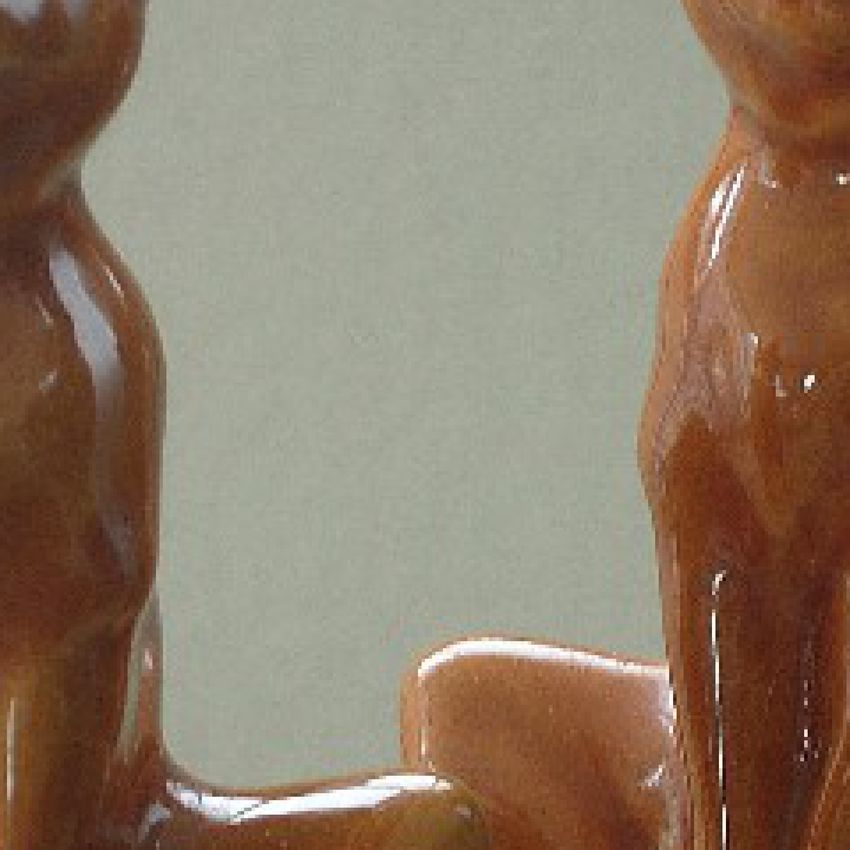
Angular Visual Hardness
1e-4
Freq=[0.0, 0.2] 10.0 Freq=[0.0, 0.2]
90 Freq=[0.2, 0.4] Freq=[0.2, 0.4]
0.6
Freq=[0.4, 0.6] Freq=[0.4, 0.6]
80 Freq=[0.6, 0.8] 9.5 Freq=[0.6, 0.8]
Freq=[0.8, 1.0] 0.5 Freq=[0.8, 1.0]
Model Accuracy
70
AVH(x)
0.4
60 9.0
||x||
50 0.3
8.5
40
0.2
Freq=[0.0, 0.2]
30 Freq=[0.2, 0.4]
8.0 0.1
Freq=[0.4, 0.6]
20 Freq=[0.6, 0.8]
Freq=[0.8, 1.0] 0.0
0 20 40 60 80 0 20 40 60 80 0 20 40 60 80
Epoch Epoch Epoch
1e-4
60 Freq=[0.0, 0.2] 10.0 Freq=[0.0, 0.2] 0.8
Freq=[0.2, 0.4] Freq=[0.2, 0.4]
Freq=[0.4, 0.6] Freq=[0.4, 0.6] 0.7
9.5
Freq=[0.6, 0.8] Freq=[0.6, 0.8]
50
Freq=[0.8, 1.0] Freq=[0.8, 1.0] 0.6
Model Accuracy
9.0
AVH(x) 0.5
40
8.5
||x||
0.4
30 8.0 0.3
0.2 Freq=[0.0, 0.2]
7.5
Freq=[0.2, 0.4]
20 Freq=[0.4, 0.6]
0.1
7.0 Freq=[0.6, 0.8]
0.0 Freq=[0.8, 1.0]
0 20 40 60 80 0 20 40 60 80 0 20 40 60 80
Epoch Epoch Epoch
1e-4
Freq=[0.0, 0.2] Freq=[0.0, 0.2] Freq=[0.0, 0.2]
9.5 0.8
Freq=[0.2, 0.4] Freq=[0.2, 0.4] Freq=[0.2, 0.4]
Freq=[0.4, 0.6] Freq=[0.4, 0.6] Freq=[0.4, 0.6]
30 Freq=[0.6, 0.8] 0.7 Freq=[0.6, 0.8]
9.0 Freq=[0.6, 0.8]
Freq=[0.8, 1.0] Freq=[0.8, 1.0] Freq=[0.8, 1.0]
Model Accuracy
0.6
8.5
AVH(x)
25
0.5
||x||
8.0
0.4
20
7.5
0.3
7.0 0.2
15
0.1
6.5
0 20 40 60 80 0 20 40 60 80 0 20 40 60 80
Epoch Epoch Epoch
1e-4
Freq=[0.0, 0.2] Freq=[0.0, 0.2] Freq=[0.0, 0.2]
Freq=[0.2, 0.4] 9.5 Freq=[0.2, 0.4] 0.8 Freq=[0.2, 0.4]
30
Freq=[0.4, 0.6] Freq=[0.4, 0.6] Freq=[0.4, 0.6]
Freq=[0.6, 0.8] Freq=[0.6, 0.8] 0.7 Freq=[0.6, 0.8]
9.0
Freq=[0.8, 1.0] Freq=[0.8, 1.0] Freq=[0.8, 1.0]
Model Accuracy
0.6
25 8.5
AVH(x)
0.5
||x||
8.0
0.4
20
7.5 0.3
15 0.2
7.0
0.1
0 20 40 60 80 0 20 40 60 80 0 20 40 60 80
Epoch Epoch Epoch
Figure 4. The left four plots show the number of Epochs v.s. Average `2 norm across ImageNet validation samples which are split into
five bins based on HSF information. The middle three plots represent number of Epochs v.s. Average AVH(x). The right ones present
number of Epochs v.s. Model Accuracy. From top to bottom, we use AlexNet, VGG-19, ResNet-50 and DenseNet-121. The shadow for
the figures in the first two columns denotes the corresponding standard deviations.
good at capturing such information (Liu et al., 2018b). This softmax score indicating the input sample hardness. We also
also justifies our angular based design as an inductive bias perform a simulation providing visual intuition of how AVH
towards measuring human visual hardness. instead of feature embedding norms corresponds to visually
hard examples on two Gaussians in Figure 7 (simulation
The AVH score is inspired by the observation from Figure 2 details and analyses in Appendix A).
as well as (Liu et al., 2018b) that samples from each class
concentrate in a convex cone in the embedding space along 3.2. Observations and Conjecture
with some interesting theoretical results that are discussed Setup. We aim to observe the complete training dynam-
above. Naturally, we conjecture AVH, a measure with angle ics of models that are trained from scratch on ImageNet
or margin information, could be the useful component of instead of the pretrained models. Therefore, we follow the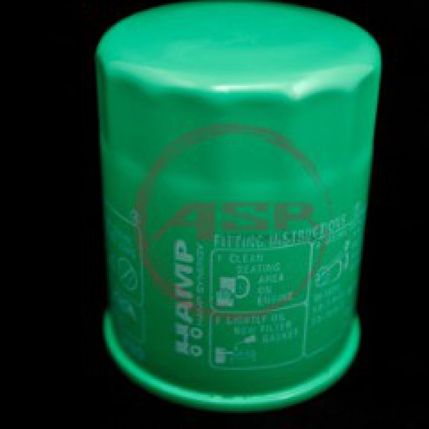
Angular Visual Hardness

standard training process of AlexNet (Krizhevsky et al.,               a plateau in all three learning rate decay stages. But the
2012), VGG-19 (Simonyan & Zisserman, 2014), ResNet-                    common observation is that they all stop improving even
50 (He et al., 2016) and DenseNet-121 (Huang et al.,                   when kxk2 and model accuracy are increasing. AVH is
2017). For consistency, we train all models for 90 epochs              more important than kxk2 in the sense that it is the key
and decay the initial learning rate by a factor of 10 ev-              factor deciding which class the input sample is classified to.
ery 30 epochs. The initial learning rate for AlexNet and               However, optimizing the norm under the current softmax
VGG-19 is 0.01 and for DenseNet-121 and ResNet-50                      cross-entropy loss would be easier, which cause the plateau
is 0.1. We split all the validation images into 5 bins,                of angles for easy examples. However, the plateau for the
[0.0, 0.2], [0.2, 0.4], [0.4, 0.6], [0.6, 0.8], [0.8, 1.0], based on   hard examples can be caused by the limitation of the model
their HSF respectively. In Appendix B, we further provide              itself and we show a simple illustration in Appendix C. It
experimental results on different datasets, such as MNIST,             shows the necessity of designing loss functions that focus
CIFAR10/100, and degraded ImageNet with different con-                 on optimizing angles.
trast or noise level, to better validate our proposal. For all
                                                                       Observation 3: AVH’s correlation with human selection
the figures in this section, epoch starts from 1.
                                                                       frequency consistently holds across models throughout
Optimization algorithms are used to update weights and bi-             the training process.
ases, i.e., the internal parameters of a model to improve the
                                                                       In Figure 4, we average over validation samples in five HSF
training loss. Both the angles between the feature embed-
                                                                       bins or five degradation level bins separately , and then
ding and classifiers, and the L2 norm of the embedding can
                                                                       compute the average embedding norm, AVH and model ac-
influence the loss. While it is well-known that the training
                                                                       curacies. We can observe that for kxk2 , the gaps between
loss or accuracy keeps improving but it is not obvious what
                                                                       the samples with different human visual hardness are not ob-
would be the dynamics of the angles and norms separately
                                                                       vious in ResNet and DenseNet, while they are quite obvious
during training. we design the experiments to observe the
                                                                       in AlexNet and VGG. However, for AVH, such AVH gaps
training dynamics of various network architectures.
                                                                       are very significant and consistent across every network ar-
Observation 1: The norm of feature embeddings keeps                    chitecture during the entire training process. Interestingly,
increasing during training.                                            even if the network is far from being converged, such AVH
                                                                       gaps are still consistent across different HSF. Also the norm
First row of Figure 4 present the dynamics of the aver-                gaps are also consistent. The intuition behind this could
age kxk2 and the dynamics of the accuracy for validation               be that the angles for hard examples are much harder to
samples vary in 90 epochs during the training on three ar-             decrease and probably never in the region for correct clas-
chitectures. Note that we are using the validation data for            sification. Therefore the corresponding norms would not
dynamics observation and therefore have never fit them into            increase otherwise hurting the loss. It validates that AVH
the model. The average kxk2 increases with a small initial             is a consistent and robust measure for visual hardness (and
slope but it suddenly climbs after 30 epochs when the first            even generalization).
learning rate decay happens. The accuracy curve is very
similar to that of the average kxk2 . These observations are           Observation 4: AVH is an indicator of a model’s gener-
consistent in all models and compatible with (Soudry et al.,           alization ability.
2018) although it is more about the norm of the classifier             From Figure 4, we observe that better models (i.e., higher
weights. More interestingly, we find that neural networks              accuracy) have lower average AVH throughout the training
with shortcuts (e.g., ResNets and DenseNets) tend to make              process and also across samples under different human vi-
the norm of the images with different HSF the same, while              sual hardness. For instance, Alexnet is the weakest model,
neural networks without shortcuts (e.g., AlexNet and VGG)              and its overall average AVH and average AVH on each of
tend to keep the gap of norm among the images with differ-             the five bins are higher than those of the other three models.
ent human visual hardness.                                             In addition, we have found that when testing Hypothesis 3
Observation 2: AVH hits a plateau very early even when                 for better models, their AVH correlations with HSF are sig-
the accuracy or loss is still improving.                               nificantly stronger than correlations of Model Confidence.
                                                                       The above observations are aligned with earlier observations
Middle row of Figure 4 exhibits the change of average AVH              from (Recht et al., 2019) that better models also tend to gen-
for validation samples in 90 epochs of training on three               eralize better on samples across different levels of human
models. The average AVH for AlexNet and VGG-19 de-                     visual hardness. In addition, AVH is potentially a better
creases sharply at the beginning and then starts to bounce             measure for the generalization of a pretrained model As
back a little bit before converging. However, the dynamics             shown in (Liu et al., 2017b), the norms of feature embed-
of the average AVH for DenseNet-121 and ResNet-50 are                  dings are often related to training data priors such as data
different. They both decrease slightly and then quickly hits           imbalance and class granularity (Krizhevsky et al., 2012).
Angular Visual Hardness
1.0 1.0 1.0
800
600 200
700
0.8 0.8 0.8 175
500
# of Samples
# of Samples
# of Samples
600
Model Confidence
150
AVH(x)
0.6 400 0.6 500 0.6
125
||x||
400
300 100
0.4 0.4 0.4
300 75
200
200 50
0.2 0.2 0.2
100
100 25
0.0 0 0.0 0 0.0 0
0.0 0.2 0.4 0.6 0.8 1.0 0.0 0.2 0.4 0.6 0.8 1.0 0.0 0.2 0.4 0.6 0.8 1.0
Human Selection Frequency Human Selection Frequency Human Selection Frequency
Figure 5. The left one presents HSF v.s. AVH(x), which we can see strong correlation. The second plot presents the correlation between
HSF and Model Confidence with ResNet-50. It is not surprising that the density is highest on the right corner. The third one presents HSF
v.s. kxk2 . There are no obvious correlation between them. Note that different color indicates the density of samples in that bin.
Table 1. presents the spearman rank correlations between HSF and AVH, Model Confidence and L2 Norm of the Embedding in ResNet-50
for different visual hardness bin of samples. Note that here we show the absolute value of the coefficient which represents the strength of
the correlation. For example, [0, 0.2] denotes the samples that have HSF from 0 to 0.2.
z-score Total Coef [0, 0.2] [0.2, 0.4] [0.4, 0.6] [0.6, 0.8] [0.8, 1.0]
Number of Samples - 29987 837 2732 6541 11066 8811
AVH 0.377 0.36 0.228 0.125 0.124 0.103 0.094
Model Confidence 0.337 0.325 0.192 0.122 0.102 0.078 0.056
kxk2 - 0.0017 0.0013 0.0007 0.0005 0.0004 0.0003
However, when extracting features from unseen classes that human visual hardness and model uncertainty is usually
do not exist in the training set, such training data prior is prohibitive because it is laborious to collect such highly
often undesired. Since AVH does not consider such feature subjective human annotations. In addition, these annota-
embedding norms, it potentially presents a better measure tions are application or dataset specific, which significantly
towards the open set generalization of a deep network. reduces the scalability of uncertainty estimation models that
are directly supervised by them. This makes yet another
Conjecture on training dynamics of CNNs. From Fig-
motivation to this work since AVH is naturally obtained for
ure 4 and observations above, we conjecture that the training
free without any confidence supervision. In our case, we
of CNN has two phases. 1) At the beginning of the training,
only leverage such human annotated visual hardness mea-
the softmax cross-entropy loss will first optimize the angles
sure for correlation testing. In this section, We first provide
among different classes while the norm will fluctuate and
four hypothesis and test them accordingly.
increase very slowly. We argue that it is because changing
the norm will not decrease the loss when the angles are not Hypothesis 1. AVH has a correlation with Human Selection
separated enough for correct classification. As a result, the Frequency.
angles get optimized firstly. 2) As the training continues, the Outcome: Null Hypothesis Rejected
angles become more stable and change very slowly while
the norm increases rapidly. On the one hand, for easy exam- We use the pre-trained network model to extract the fea-
ples, it is because when the angles get decreased enough for ture embedding x from each validation sample and also
correct classification, the softmax cross-entropy loss can be provide the class weights w to compute AVH(x). Note
well minimized by purely increasing the norm. On the other that we linearly scale the range of AVH(x) to [0, 1]. Ta-
hand, for hard examples, the plateau is caused by that the ble 1 shows the overall consistent and stronger correlation
CNN is unable to decrease the angle to correctly classify between AVH(x) and HSF (p-value is < 0.001 rejecting
examples and thereby also unable to increase the norms the null hypothesis). From the coefficients shown in dif-
(because it may otherwise increase the loss). ferent bins of sample hardness, we can see that the harder
the sample, the weaker the correlation. Also Note that we
4. Connections to Human Visual Hardness validate the results across different CNN architectures and
found that better models tend to have higher coefficients.
From Section 3.2, we conjecture that AVH has a stronger
correlation with human selection frequency - a reflection of The plot on the left in Figure 5 indicates the strong correla-
human visual hardness that is related to aleatoric uncertainty. tion between AVH(x) and HSF on validation images. One
In order to validate this claim, we design statistical testings intuition behind this correlation is that the class weights W
for the connections between Model Confidence, AVH, kxk2 might correspond to human perceived semantics for each
and HSF. Studying the precise connection or gap between category and thereby AVH(x) corresponds to human’s se-Angular Visual Hardness
Table 2. presents the spearman rank, Pearson, and Kendall Tau correlations between human selection frequency and AVH, Model
Confidence in ResNet50 along with the significance testing between coefficient pairs. Note that p-value< 0.05 represents the result is
significant.
Coef with AVH Coef with Model Confidence Zavh Zmc Z value p-value
Spearman 0.360 0.325 0.377 0.337 4.85 < .00001
Pearson 0.385 0.341 0.406 0.355 6.2 < .00001
Kendall Tau 0.257 0.231 0.263 0.235 3.38 .0003
mantic categorization of an image. In order to test if the of AVH becomes 0.377 and that of Model Confidence be-
strong correlation holds for all models, we perform the comes 0.337. The second step is to compute the Z value of
same set of experiments on different backbones, including two Z scores. Then we determined the Z value to be 4.85
AlexNet, VGG-19 and DenseNet-121. from the two above-mentioned Z scores and sample sizes.
Hypothesis 2. Model Confidence has a correlation with The last step is that find out the p-value according to the Z
Human Selection Frequency. table. According to Z table, p-value is 0.00001. Therefore,
we reject the null hypothesis and conclude that AVH has
Outcome: Null Hypothesis Rejected statistically significant stronger correlation with HSF than
Model Confidence. In later section 5.1, we also empiri-
An interesting observation in (Recht et al., 2019) shows
cally show that such stronger correlation brings cumulative
that HSF has strong influence on the Model Confidence.
advantages in some applications.
Specifically, examples with low HSF tends to have rela-
tively low Model Confidence. Naturally we examine if the In table 2, besides the Spearman correlation coefficient, we
correlation between Model Confidence and HSF is strong. also show the coefficients of Pearson and Kendall Tau. In
Specifically, all ImageNet validation images are evaluated addition, in Appendix D, we run the same tests on four
by the pre-trained models. The corresponding output is sim- different architectures to test whether the same conclusion
ply the Model Confidence on each image. From table 1, we holds for different models. Our conclusion is that for all the
can first see that it is clear that because p-value is < 0.001, considered models, AVH correlates significantly stronger
Model Confidence does have a strong correlation with HSF. than Model Confidence, and the correlation is even stronger
However, the correlation coefficient for Model Confidence for better models. This indicates that besides what we have
and HSF is consistently lower than that of AVH and HSF. shown in section 3, AVH is also better aligned with human
visual hardness which is related to aleatoric uncertainty.
The middle plot in figure 5 presents a two-dimensional
histogram for the correlation visualization. The x-axis rep- Hypothesis 4. kxk2 has a correlation with Human Selec-
resents HSF, and the y-axis represents Model Confidence. tion Frequency.
Each bin exhibits the number of images which lie in the
corresponding range. We can observe the high density at
Outcome: Failure to Reject Null Hypothesis
the right corner, which means the majority of the images
have both high human and model accuracy. However, there (Liu et al., 2018b) conjectures that kxk2 accounts for intra-
is a considerable amount of density on the range of medium class Human/Model Confidence. Particularly, if the norm is
human accuracy but either extremely low or high model larger, the prediction from the model is also more confident,
accuracy. One may question that the difference of the corre- to some extent. Therefore, we conduct similar experiments
lation coefficient is not large, thereby we also run statistical like previous section to demonstrate the correlation between
testing on the significance of the gap, naturally our next step kxk2 and HSF. Initially, we compute the kxk2 for every
is to test if the difference is significant. validation sample for all models. Then we normalize kxk2
Hypothesis 3. AVH has a stronger correlation to Human within each class. Table 1 presents the results for the corre-
Selection Frequency than Model Confidence. lation test. We omit the results for p-value in the table and
report here that they are all much higher than 0.05, indicat-
Outcome: Null Hypothesis Rejected ing there is no correlation between kxk2 and HSF. The right
plot in figure 5 uses a two-dimensional histogram to show
There are three steps for testing if two correlation coef-
the correlation for all the validation images. Given that the
ficient are significantly different. First step is applying
norm has been normalized with each class, naturally, there
Fisher Z-Transformation to both coefficients. The Fisher
is notable density when the norm is 0 or 1. Except for that,
Z-Transformation is a way to transform the sampling dis-
there is no obvious correlation between kxk2 and HSF.
tribution of the correlation coefficient so that it becomes
normally distributed. Therefore, we apply fisher transforma- We also provide a detailed discussion on the difference
tion for each correlation coefficient: Z score for coefficient between AVH and Model Confidence in Appendix E.Angular Visual Hardness
5. Applications Ŷ alternatively, and the solver of Ŷ can be written as:
8
5.1. AVH for Self-training and Domain Adaptation k
(k)⇤
ŷt = k k
:
Unsupervised domain adaptation (Ben-David et al., 2010) 0, otherwise
presents an important transfer learning problem and deep
self-training (Lee, 2013) recently emerged as a powerful The optimization with respect to w is simply network re-
framework to this problem (Saito et al., 2017a; Shu et al., training with source labels and estimated pseudo-labels. The
2018; Zou et al., 2018; 2019). Here we show the application complete self-training process involves alternative repeat of
of AVH as an improved confidence measure in self-training network re-training and pseudo-label estimation.
that could significantly benefit domain adaptation. CBST+AVH: We seek to improve the pseudo-label solver
Dataset: We conduct expeirments on the VisDA-17 (Peng with better confidence measure from AVH. We propose the
et al., 2017) dataset which is a widely used major benchmark following definition of angular visual confidence (AVC) to
for domain adaptation in image classification. The dataset represent the predicted probability of class c:
contains a total number of 152, 409 2D synthetic images ⇡ A(x, wc )
AVC(c|x; w) = PK , (3)
from 12 categories in the source training set, and 55, 400 k=1 (⇡ A(x, wk ))
real images from MS-COCO (Lin et al., 2014) with the
same set of categories as the target domain validation set. and pseudo-label estimation in CBST+AVH is defined as:
8
We follow the protocol of previous works to train a source > AVC(k|xt ; w)
>
model with the synthetic training set, and report the model
k k
}
(k)⇤
performance on target validation set upon adaptation. ŷt = (4)
>
> and AVC(k|xt ; w) > k
>
:
Baseline: We use class-balanced self-training (CBST) (Zou 0, otherwise
et al., 2018) as a state-of-the-art self-training baseline. We
where k is differently determined by referring to
also compare our model with confidence regularized self-
AV C(k|xt ; w) ranked at portion p among samples pre-
training (CRST)1 (Zou et al., 2019), a more recent frame-
dicted to class k by AVH, following a similar definition of
work improved over CBST with network prediction/pseudo-
k in CBST. In addition, network re-training in CBST+AVH
label regularized with smoothness. Specifically, our work
follows the softmax self-training loss in (2).
follows the exact implementation of CBST/CRST.
One could see that AVH changes the self-training behavior
Specifically, given the labeled source domain training set
from two ways with the conditions in (4):
xs 2 XS and the unlabeled target domain data xt 2 XT ,
(1) (K) Improved selection: AV C(k|xt ; w) > k .
with known source labels ys = (ys , ..., ys ) 2 YS and
(1) (K) Improved classification: k = arg maxk { AV C(k|x t ;w)
}.
unknown target labels ŷt = (ŷt , ..., ŷt ) 2 ŶT from K k
Specifically, the former determines which samples are not
classes, CBST performs joint network learning and pseudo- ignored during self-training based on AVC, whereas the lat-
label estimation by treating pseudo-labels as discrete learn- ter determines the pseudo-label class by taking argmax over
able latent variables with the following loss: normalized AVC scores. With improved confidence measure
K
XX that better resembles human visual hardness, both aspects
min LCB (w, Ŷ) = ys(k) log p(k|xs ; w) are likely to influence the performance of self-training.
w,ŶT
s2S k=1
(2)
K
XX (k) p(k|xt ; w) K
Experimental Results: We present the results of the pro-
ŷt log s.t. ŷt 2 E [ {0}, 8t posed method in Table 3, and also show its performance
k
t2T k=1
with respect to different self-training epochs in Figure 6.
where the feasible set of pseudo-labels is the union of {0} One could see that CBST+AVH outperforms both CBST
and the K dimensional one-hot vector space EK , and w and and CRST by a very significant margin. We would like to
p(k|x; w) represent the network weights and the classifier’s emphasize that this is a very compelling result under “ap-
softmax probability for class k, respectively. In addition, k ples to apples” comparison with the same source model,
serves as a class-balancing parameter controlling the pseudo- implementation and hyper-parameters.
label selection of class k, and is determined by the softmax
Analysis: A major challenge of self-training is the ampli-
confidence ranked at portion p (in descending order) among
fication of error due to misclassified pseudo-labels. There-
samples predicted to class k. Therefore, only one parameter
fore, traditional self-training methods such as CBST often
p is used to determine all k ’s. The optimization problem
use model confidence as the measure to select confidently
in (2) can be solved via minimizing with respect to w and
labeled examples. The hope is that higher confidence poten-
1
We consider MRKLD+LRENT which is reported to be the tially implies lower error rate. While this generally proves
highest one in (Zou et al., 2019). useful, the model tends to focus on the “less informative”Angular Visual Hardness
Table 3. Class-wise and mean classification accuracies on VisDA-17.
Method Aero Bike Bus Car Horse Knife Motor Person Plant Skateboard Train Truck Mean
Source (Saito et al., 2018) 55.1 53.3 61.9 59.1 80.6 17.9 79.7 31.2 81.0 26.5 73.5 8.5 52.4
MMD (Long et al., 2015b) 87.1 63.0 76.5 42.0 90.3 42.9 85.9 53.1 49.7 36.3 85.8 20.7 61.1
DANN (Ganin et al., 2016) 81.9 77.7 82.8 44.3 81.2 29.5 65.1 28.6 51.9 54.6 82.8 7.8 57.4
ENT (Grandvalet & Bengio, 2005) 80.3 75.5 75.8 48.3 77.9 27.3 69.7 40.2 46.5 46.6 79.3 16.0 57.0
MCD (Saito et al., 2017b) 87.0 60.9 83.7 64.0 88.9 79.6 84.7 76.9 88.6 40.3 83.0 25.8 71.9
ADR (Saito et al., 2018) 87.8 79.5 83.7 65.3 92.3 61.8 88.9 73.2 87.8 60.0 85.5 32.3 74.8
Source (Zou et al., 2019) 68.7 36.7 61.3 70.4 67.9 5.9 82.6 25.5 75.6 29.4 83.8 10.9 51.6
CBST (Zou et al., 2019) 87.2 78.8 56.5 55.4 85.1 79.2 83.8 77.7 82.8 88.8 69.0 72.0 76.4
CRST (Zou et al., 2019) 88.0 79.2 61.0 60.0 87.5 81.4 86.3 78.8 85.6 86.6 73.9 68.8 78.1
Proposed 93.3 80.2 78.9 60.9 88.4 89.7 88.9 79.6 89.5 86.8 81.5 60.0 81.5
Table 5. Domain generalization accuracy (%) on PACS dataset.
80
Method Painting Cartoon Photo Sketch Avg
75
AlexNet (Li et al., 2017) 62.86 66.97 89.50 57.51 69.21
MLDG (Li et al., 2018) 66.23 66.88 88.00 58.96 70.01
Accuracy
70
MetaReg (Balaji et al., 2018) 69.82 70.35 91.07 59.26 72.62
65 Feature-critic (Li et al., 2019) 64.89 71.72 89.94 61.85 72.10
Baseline CNN-10 66.46 67.88 89.70 51.72 68.94
60
CBST + AVH
CNN-10 + AVH 72.02 66.42 90.12 61.26 72.46
55
CRST
CBST
5.0 7.5 10.0 12.5 15.0 17.5 20.0 depend on the generalizability of the neural network. We
Epoch use the challenging PACS dataset (Li et al., 2017) which
Figure 6. Adaptation accuracy vs. epoch for different comparing consists of Art painting, Cartoon, Photo and Sketch domains.
methods on VisDA-17. For each domain, we leave it out as the test set and train our
models on rest of the three domains.
Table 4. Statistics of the examples selected by CBST+AVH and
Specifically, we train a 10-layer plain CNN with the follow-
CBST/CRST.
TP Rate AVH (avg) Model Confidence Norm kxk
ing AVH-based loss (additional details in Appendix F):
CBST+AVH 0.844 0.118 0.961 20.84 X
CBST/CRST 0.848 0.117 0.976 21.28
exp s(⇡ A(xi , wyi ))
LAV H = PK , (5)
i k=1 exp s(⇡ A(xi , wk ))
samples, whereas ignoring the “more informative”, harder
ones near classier boundaries that could be essential for where s is hyperparameter that adjusts the scale of the out-
learning a better classifier. More details are in Appendix F. put logits and implicitly controls the optimization difficulty.
This hyperparameter is typically set by cross-validation. Ex-
An advantage we observe from AVH is that the improved cal- perimental results are reported in Table 5. With the proposed
ibration leads to more frequent sampling of harder samples, new loss which directly has an AVH-based design, a simple
whereas the pseudo-label classification on these hard sam- CNN is outperforming baseline and recent methods that are
ples generally outperforms softmax results. Table 4 shows based on more complex models. In fact, similar learning
the statistics of examples selected with AVH and model con- objectives have also been shown useful in image recogni-
fidence respectively at the beginning of the training process. tion (Liu et al., 2017c) and face recognition (Wang et al.,
The true positive rate (TP Rate) for CBST+AVH remains 2017; Ranjan et al., 2017), indicating that AVH is generally
similar to CBST/CRST, indicating AVH overall is not intro- effective to improve generalization in various tasks.
ducing additional noise compare to model confidence. On
the other hand, it is observed that the average model confi- 6. Concluding Remarks
dence of AVH selected samples is lower, indicating there are
more selected hard samples that are closer to the decision We propose a novel measure for CNN models known as an-
boundary. It is also observed that the average sample norm gular visual hardness. Our comprehensive empirical studies
by AVH is also lower, confirming the influence of sample show that AVH can serve as an indicator of generalization
norms on ultimate model confidence. abilities of neural networks, and improving SOTA accuracy
entails improving accuracy on hard examples. AVH also
has a significantly stronger correlation with human selection
5.2. AVH-based loss for Domain Generalization
frequency. We empirically show the huge advantage of AVH
The problem of domain generalization (DG) is to learn from over Model Confidence in self-training for domain adapta-
multiple training domains, and extract a domain-agnostic tion task and loss function for domain generalization task.
model that can then be applied to an unseen domain. Since AVH can be useful in other applications such as deep metric
we have no assumption on how the unseen domain looks learning, fairness, knowledge transfer, etc. and we plan to
like, the generalization on the unseen domains will mostly investigate them in the future (discussions in Appendix G).Angular Visual Hardness
Acknowledgements Finn, C., Abbeel, P., and Levine, S. Model-agnostic meta-
learning for fast adaptation of deep networks. In ICML,
We would like to thank Shiyu Liang, Yue Zhu and Yang 2017.
Zou for the valuable discussions that enlighten our re-
search. We are also grateful to the anonymous reviewers Gal, Y. and Ghahramani, Z. Dropout as a bayesian approxi-
for their constructive comments that significantly helped mation: Representing model uncertainty in deep learning.
to improve our paper. Weiyang Liu is partially supported In ICML, 2016.
by Baidu scholarship and NVIDIA GPU grant. This work
was supported by NSF-1652131, NSF-BIGDATA 1838177, Gal, Y., Hron, J., and Kendall, A. Concrete dropout. In
AFOSR-YIPFA9550-18-1-0152, Amazon Research Award, NeurIPS, 2017.
and ONR BRC grant for Randomized Numerical Linear
Ganin, Y., Ustinova, E., Ajakan, H., Germain, P., Larochelle,
Algebra.
H., Laviolette, F., Marchand, M., and Lempitsky, V.
Domain-adversarial training of neural networks. JMLR,
References 2016.
Balaji, Y., Sankaranarayanan, S., and Chellappa, R. Metareg: Geirhos, R., Temme, C. R., Rauber, J., Schütt, H. H., Bethge,
Towards domain generalization using meta-regularization. M., and Wichmann, F. A. Generalisation in humans and
In NeurIPS, 2018. deep neural networks. In Advances in Neural Information
Ben-David, S., Blitzer, J., Crammer, K., Kulesza, A., Processing Systems, pp. 7538–7550, 2018.
Pereira, F., and Vaughan, J. W. A theory of learning from
Geirhos, R., Rubisch, P., Michaelis, C., Bethge, M., Wich-
different domains. Machine learning, 79(1-2):151–175,
mann, F. A., and Brendel, W. Imagenet-trained cnns are
2010.
biased towards texture; increasing shape bias improves
Bengio, Y., Louradour, J., Collobert, R., and Weston, J. accuracy and robustness. 2019.
Curriculum learning. In ICML, 2009.
Goodfellow, I. J., Shlens, J., and Szegedy, C. Explain-
Berardino, A., Ballé, J., Laparra, V., and Simoncelli, E. P. ing and harnessing adversarial examples. arXiv preprint
Eigen-distortions of hierarchical representations, 2017. arXiv:1412.6572, 2014.
Buolamwini, J. and Gebru, T. Gender shades: Intersectional Grandvalet, Y. and Bengio, Y. Semi-supervised learning by
accuracy disparities in commercial gender classification. entropy minimization. In NeurIPS, 2005.
In Conference on Fairness, Accountability and Trans-
parency, pp. 77–91, 2018. Guo, C., Pleiss, G., Sun, Y., and Weinberger, K. Q. On
calibration of modern neural networks. In Proceedings of
Chen, M., Weinberger, K. Q., and Blitzer, J. Co-training for the 34th International Conference on Machine Learning-
domain adaptation. In Advances in neural information Volume 70, pp. 1321–1330. JMLR. org, 2017.
processing systems, pp. 2456–2464, 2011.
Hadsell, R., Chopra, S., and LeCun, Y. Dimensionality
Dekel, R. Human perception in computer vision, 2017. reduction by learning an invariant mapping. In CVPR,
Deng, J., Dong, W., Socher, R., Li, L.-J., Li, K., and Fei-Fei, 2006.
L. Imagenet: A large-scale hierarchical image database. Hariharan, B. and Girshick, R. Low-shot visual recognition
In CVPR, 2009. by shrinking and hallucinating features. In ICCV, 2017.
Deng, J., Guo, J., Xue, N., and Zafeiriou, S. Arcface:
He, K., Zhang, X., Ren, S., and Sun, J. Deep residual learn-
Additive angular margin loss for deep face recognition.
ing for image recognition. In Proceedings of the IEEE
In CVPR, 2019.
conference on computer vision and pattern recognition,
Der Kiureghian, A. and Ditlevsen, O. Aleatory or epistemic? pp. 770–778, 2016.
does it matter? Structural safety, 31(2):105–112, 2009.
Hinton, G., Vinyals, O., and Dean, J. Distilling
Dodge, S. and Karam, L. A study and comparison of human the knowledge in a neural network. arXiv preprint
and deep learning recognition performance under visual arXiv:1503.02531, 2015.
distortions. 2017 26th International Conference on Com-
puter Communication and Networks (ICCCN), Jul 2017. Huang, G., Liu, Z., Van Der Maaten, L., and Weinberger,
doi: 10.1109/icccn.2017.8038465. K. Q. Densely connected convolutional networks. In
Proceedings of the IEEE conference on computer vision
Fellbaum, C. Wordnet and wordnets. 2005. and pattern recognition, pp. 4700–4708, 2017.Angular Visual Hardness
Kendall, A. and Gal, Y. What uncertainties do we need in Lin, T.-Y., Maire, M., Belongie, S., Hays, J., Perona, P., Ra-
bayesian deep learning for computer vision? In NeurIPS, manan, D., Dollár, P., and Zitnick, C. L. Microsoft coco:
2017. Common objects in context. In European conference on
computer vision, pp. 740–755. Springer, 2014.
Kheradpisheh, S. R., Ghodrati, M., Ganjtabesh, M., and
Masquelier, T. Deep networks can resemble human feed- Lindsay, P. H. and Norman, D. A. Human information
forward vision in invariant object recognition. Scientific processing: An introduction to psychology. Academic
Reports, 6(1), Sep 2016. ISSN 2045-2322. doi: 10.1038/ press, 2013.
srep32672. Liu, W., Wen, Y., Yu, Z., and Yang, M. Large-margin
softmax loss for convolutional neural networks. In ICML,
Krizhevsky, A., Sutskever, I., and Hinton, G. E. Imagenet
2016.
classification with deep convolutional neural networks.
In Advances in neural information processing systems, Liu, W., Dai, B., Humayun, A., Tay, C., Yu, C., Smith, L. B.,
pp. 1097–1105, 2012. Rehg, J. M., and Song, L. Iterative machine teaching. In
ICML, 2017a.
Kumar, A., Sarawagi, S., and Jain, U. Trainable calibration
measures for neural networks from kernel mean embed- Liu, W., Wen, Y., Yu, Z., Li, M., Raj, B., and Song, L.
dings. In International Conference on Machine Learning, Sphereface: Deep hypersphere embedding for face recog-
pp. 2810–2819, 2018. nition. In CVPR, 2017b.
Liu, W., Zhang, Y.-M., Li, X., Yu, Z., Dai, B., Zhao, T.,
Kumar, M. P., Packer, B., and Koller, D. Self-paced learning
and Song, L. Deep hyperspherical learning. In NeurIPS,
for latent variable models. In NeurIPS, 2010.
2017c.
Lakshminarayanan, B., Pritzel, A., and Blundell, C. Simple Liu, W., Lin, R., Liu, Z., Liu, L., Yu, Z., Dai, B., and Song,
and scalable predictive uncertainty estimation using deep L. Learning towards minimum hyperspherical energy. In
ensembles. In Guyon, I., Luxburg, U. V., Bengio, S., Wal- NeurIPS, 2018a.
lach, H., Fergus, R., Vishwanathan, S., and Garnett, R.
(eds.), Advances in Neural Information Processing Sys- Liu, W., Liu, Z., Yu, Z., Dai, B., Lin, R., Wang, Y., Rehg,
tems 30, pp. 6402–6413. Curran Associates, Inc., 2017. J. M., and Song, L. Decoupled networks. In CVPR,
2018b.
Lee, D.-H. Pseudo-label: The simple and efficient semi-
supervised learning method for deep neural networks. In Liu, W., Liu, Z., Rehg, J. M., and Song, L. Neural similarity
ICML Workshop on Challenges in Representation Learn- learning. In NeurIPS, 2019.
ing, 2013. Liu, W., Lin, R., Liu, Z., Rehg, J. M., Xiong, L., Weller,
A., and Song, L. Orthogonal over-parameterized training.
Li, D., Yang, Y., Song, Y.-Z., and Hospedales, T. M. Deeper,
arXiv preprint arXiv:2004.04690, 2020.
broader and artier domain generalization. In Proceedings
of the IEEE international conference on computer vision, Long, J., Shelhamer, E., and Darrell, T. Fully convolutional
pp. 5542–5550, 2017. networks for semantic segmentation. In CVPR, 2015a.
Li, Y., Yang, Y., Zhou, W., and Hospedales, T. M. Feature- Long, M., Cao, Y., Wang, J., and Jordan, M. I. Learning
critic networks for heterogeneous domain generalization. transferable features with deep adaptation networks. In
arXiv preprint arXiv:1901.11448, 2019. ICML, 2015b.
Martin Cichy, R., Khosla, A., Pantazis, D., and Oliva, A.
Li, Z. and Hoiem, D. Reducing over-confident errors outside
Dynamics of scene representations in the human brain
the known distribution. arXiv preprint arXiv:1804.03166,
revealed by magnetoencephalography and deep neural
2018.
networks. NeuroImage, 153:346–358, Jun 2017. ISSN
Li, Z., Xu, Z., Ramamoorthi, R., Sunkavalli, K., and Chan- 1053-8119. doi: 10.1016/j.neuroimage.2016.03.063.
draker, M. Learning to reconstruct shape and spatially- Oh Song, H., Xiang, Y., Jegelka, S., and Savarese, S. Deep
varying reflectance from a single image. In SIGGRAPH metric learning via lifted structured feature embedding.
Asia 2018 Technical Papers, pp. 269. ACM, 2018. In CVPR, 2016.
Lin, R., Liu, W., Liu, Z., Feng, C., Yu, Z., Rehg, J. M., Peng, X., Usman, B., Kaushik, N., Hoffman, J., Wang, D.,
Xiong, L., and Song, L. Regularizing neural networks via and Saenko, K. Visda: The visual domain adaptation
minimizing hyperspherical energy. In CVPR, 2020. challenge. arXiv preprint arXiv:1710.06924, 2017.Angular Visual Hardness
Pramod, R. T. and Arun, S. P. Do computational models dif- Wang, F., Xiang, X., Cheng, J., and Yuille, A. L. Normface:
fer systematically from human object perception? 2016 L2 hypersphere embedding for face verification. In ACM-
IEEE Conference on Computer Vision and Pattern Recog- MM, 2017.
nition (CVPR), Jun 2016. doi: 10.1109/cvpr.2016.177.
Wang, F., Liu, W., Liu, H., and Cheng, J. Additive
Ranjan, R., Castillo, C. D., and Chellappa, R. L2- margin softmax for face verification. arXiv preprint
constrained softmax loss for discriminative face verifica- arXiv:1801.05599, 2018a.
tion. arXiv preprint arXiv:1703.09507, 2017.
Wang, H., Wang, Y., Zhou, Z., Ji, X., Gong, D., Zhou, J.,
Recht, B., Roelofs, R., Schmidt, L., and Shankar, V. Do im- Li, Z., and Liu, W. Cosface: Large margin cosine loss for
agenet classifiers generalize to imagenet? arXiv preprint deep face recognition. In CVPR, 2018b.
arXiv:1902.10811, 2019. Wang, Y., Liu, W., Ma, X., Bailey, J., Zha, H., Song, L., and
Saito, K., Ushiku, Y., and Harada, T. Asymmetric tri- Xia, S.-T. Iterative learning with open-set noisy labels.
training for unsupervised domain adaptation. In ICML, In CVPR, 2018c.
2017a. Wang, Z., Bovik, A. C., Sheikh, H. R., and Simoncelli, E. P.
Image quality assessment: from error visibility to struc-
Saito, K., Watanabe, K., Ushiku, Y., and Harada, T. Max-
tural similarity. IEEE transactions on image processing,
imum classifier discrepancy for unsupervised domain
13(4):600–612, 2004.
adaptation. 2017b.
Wei, C. and Ma, T. Improved sample complexities for deep
Saito, K., Ushiku, Y., Harada, T., and Saenko, K. Adversar- networks and robust classification via an all-layer margin.
ial dropout regularization. In ICLR, 2018. arXiv preprint arXiv:1910.04284, 2019.
Schroff, F., Kalenichenko, D., and Philbin, J. Facenet: A Wu, C.-Y., Manmatha, R., Smola, A. J., and Krahenbuhl, P.
unified embedding for face recognition and clustering. In Sampling matters in deep embedding learning. In ICCV,
CVPR, 2015. 2017.
Shu, R., Bui, H. H., Narui, H., and Ermon, S. A dirt-t Yi, D., Lei, Z., Liao, S., and Li, S. Z. Learning face repre-
approach to unsupervised domain adaptation. 2018. sentation from scratch. arXiv preprint arXiv:1411.7923,
2014.
Simonyan, K. and Zisserman, A. Very deep convolu-
tional networks for large-scale image recognition. arXiv Zhang, R., Isola, P., Efros, A. A., Shechtman, E., and Wang,
preprint arXiv:1409.1556, 2014. O. The unreasonable effectiveness of deep features as a
perceptual metric. In Proceedings of the IEEE Conference
Sohn, K. Improved deep metric learning with multi-class on Computer Vision and Pattern Recognition, pp. 586–
n-pair loss objective. In NeurIPS, 2016. 595, 2018.
Soudry, D., Hoffer, E., Nacson, M. S., Gunasekar, S., and Zhou, B., Lapedriza, A., Xiao, J., Torralba, A., and Oliva, A.
Srebro, N. The implicit bias of gradient descent on sepa- Learning deep features for scene recognition using places
rable data. The Journal of Machine Learning Research, database. In NeurIPS, 2014.
19(1):2822–2878, 2018.
Zhou, Y., Kantarcioglu, M., and Thuraisingham, B. Self-
Springenberg, J. T., Klein, A., Falkner, S., and Hutter, F. training with selection-by-rejection. In 2012 IEEE 12th
Bayesian optimization with robust bayesian neural net- international conference on data mining, pp. 795–803.
works. In Lee, D. D., Sugiyama, M., Luxburg, U. V., IEEE, 2012.
Guyon, I., and Garnett, R. (eds.), Advances in Neural In-
Zhu, X. Semi-supervised learning tutorial.
formation Processing Systems 29, pp. 4134–4142. Curran
Associates, Inc., 2016. Zou, Y., Yu, Z., Kumar, B., and Wang, J. Domain adapta-
tion for semantic segmentation via class-balanced self-
Sun, Y., Wang, X., and Tang, X. Deep learning face rep-
training. arXiv preprint arXiv:1810.07911, 2018.
resentation from predicting 10,000 classes. In CVPR,
2014. Zou, Y., Yu, Z., Liu, X., Kumar, B., and Wang, J.
Confidence regularized self-training. arXiv preprint
Tang, P., Wang, X., Bai, X., and Liu, W. Multiple instance arXiv:1908.09822, 2019.
detection network with online instance classifier refine-
ment. In CVPR, 2017.You can also read