Metric Factorization: Recommendation beyond Matrix Factorization
←
→
Page content transcription
If your browser does not render page correctly, please read the page content below
Metric Factorization: Recommendation beyond Matrix Factorization

                                                          Shuai Zhang∗ , Lina Yao∗ , Yi Tay† , Xiwei Xu‡ , Xiang Zhang∗ and Liming Zhu‡
                                                                               ∗ Schoolof Computer Science and Engineering,
                                                                                       University of New South Wales
                                                               Email: {shuai.zhang@student., lina.yao@,xiang.zhang3@student.}unsw.edu.au
                                                                              † School of Computer Science and Engineering,
                                                                                     Nanyang Technological University
                                                                                        Email: ytay017@e.ntu.edu.sg
                                                                                             ‡ Data61, CSRIO,
arXiv:1802.04606v2 [cs.IR] 4 Jun 2018

                                                                             Email: {Xiwei.Xu, Liming.Zhu}@data61.csrio.au

                                        Abstract—In the past decade, matrix factorization has been        (e.g., 1 to 5) of unrated items to which users may likely
                                        extensively researched and has become one of the most popular     give based on observed explicit ratings. Many well-known
                                        techniques for personalized recommendations. Nevertheless,        websites such as Netflix, Movielens, IMDB and Douban
                                        the dot product adopted in matrix factorization based rec-        collect explicit ratings which could be used as an important
                                        ommender models does not satisfy the inequality property,         indicator of user interests and preferences. In some cases
                                        which may limit their expressiveness and lead to sub-optimal      where explicit ratings are absent, rank-based recommenda-
                                        solutions. To overcome this problem, we propose a novel           tion models are more desirable and practical as abundant
                                        recommender technique dubbed as Metric Factorization. We          implicit feedback (e.g., click, view history, purchase log
                                        assume that users and items can be placed in a low dimensional    etc.) can be used for generating personalized ranked lists
                                        space and their explicit closeness can be measured using          to accomplish the recommendation goal. In this study, we
                                        Euclidean distance which satisfies the inequality property. To    will investigate the usefulness of metric factorization on both
                                        demonstrate its effectiveness, we further designed two variants   scenarios.
                                        of metric factorization with one for rating estimation and the         RS has been an active research area for both practitioners
                                        other for personalized item ranking. Extensive experiments        and researchers. Since the Netflix contest, many recom-
                                        on a number of real-world datasets show that our approach         mender systems resort to matrix factorization (MF) due to
                                        outperforms existing state-of-the-art by a large margin on both   its superior performance over non-personalized and memory
                                        rating prediction and item ranking tasks.
                                                                                                          based approaches. MF factorizes the large user-item interac-
                                                                                                          tion matrix into a product of two low-dimensional matrices.
                                                                                                          MF assumes that users and items can be represented by
                                        1. Introduction                                                   latent factors in a low dimensional space, and models their
                                                                                                          similarities with dot product. In recent years, many variants
                                            Recommender systems (RS) are among the most ubiq-             based on matrix factorization such as, SVD [1], Bayesian
                                        uitous and popular components for modern online business.         personalized ranking [2], weighted regularized matrix factor-
                                        RS aims to identify the most interesting and relevant items       ization [3], probabilistic matrix factorization [4] have been
                                        (e.g., movies, songs, products, events, articles etc.) from       developed. To some extent, MF has become a dominant
                                        a large corpus and make personalized recommendation for           pillar for building up recommender systems despite the fact
                                        each user. An increasing number of e-commerce and retail          that its performance may be hindered by the simple choice of
                                        companies are utilizing RS to promote their products, enrich      interaction method: dot product [5], [6]. It is known that dot
                                        shopping potential, boost sales and encourage customer en-        product does not satisfy the triangle inequality [7] which is
                                        gagement. For customers, RS is an essential filtering tool for    defined as: “the distance between two points cannot be larger
                                        overcoming information overload caused by unmanageable            than the sum of their distances from a third point” [8]. This
                                        amount of resources and selections. As such, RS is of great       weakness limits the expressiveness of matrix factorization
                                        value to both companies and end users, and a wide spectrum        and may result in sub-optimal solutions. Detailed explana-
                                        of recommendation models have been developed in the past          tions are provided in Section 3. Moreover, empirical studies
                                        decade.                                                           also show that matrix factorization is prone to overfitting
                                            RS predicts user’s preference on items based on their his-    for large size of latent factors, which substantially restrict
                                        torical interactions such as ratings, previous purchases and      the model flexibility and capability.
                                        click-through. In general, there mainly exist two categories           To mitigate the above mentioned problem, we propose a
                                        of recommender tasks: rating prediction and item ranking.         novel technique: Metric Factorization, which is applicable
                                        The former targets on estimating real-valued rating score         to both rating prediction and item ranking. The rational is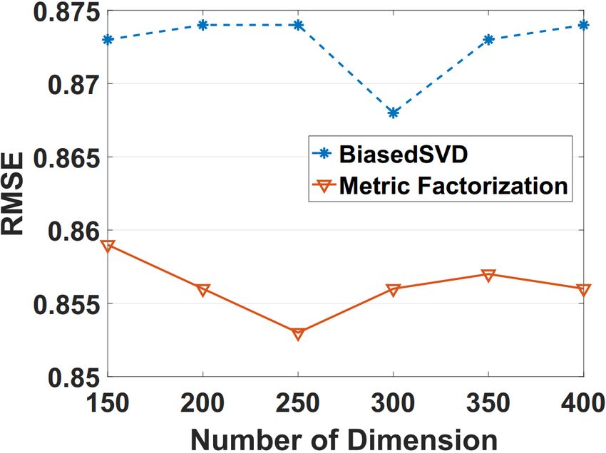
to replace the dot product of MF with Euclidean distance,         entries) of the user item interaction matrix. WRMF also has
and consider the recommendation problem from a position           a confidence value used to control the weight of negative
and distance perspective. It factorizes the interaction matrix    and positive entries. Incorporating side information into MF
into user and item dense embedding, and makes recom-              is also viable, nonetheless, this work mainly focuses on
mendations based on their estimated distances. The main           overcoming the limitation of dot product and we leave the
contributions of this work are summarized as follows:             side information modelling with metric factorization as a
                                                                  future work.
    •    We proposed a novel technique, metric factorization,
         in which users and items are represented as points            As aforementioned, despite the success of MF, it capabil-
         in a multi-dimensional coordinate system. Their dis-     ities are constrained by dot product. To this end, several at-
         tances are measured with the Euclidean distance.         tempts are made to overcome this problem. One approach is
         Recommendations are made based on user and item          to introduce non-linearity to matrix factorization [11]. Dziu-
         closeness.                                               gaite et al. [12] proposed a neural network generalization of
    •    We specify two variants of metric factorization to       matrix factorization by modeling the user-item relationships
         solve the two classic recommendation tasks: rating       with non-linear neural networks. The basic idea is to apply
         prediction and item ranking. Our model can ef-           non-linear activation functions over the element-wise prod-
         fectively learn the positions of users and items in      uct of user and item latent factors. He et al. [5] followed this
         both settings. Source code of metric factorization is    idea and proposed the neural collaborative filtering (NeuMF)
         available at Github1 .                                   model for personalized ranking task. NeuMF consists of a
    •    Extensive experiments on a wide spectrum of large        generalized MF and a multilayer perceptron. It treats the
         scale datasets demonstrate that our model outper-        one-class collaborative filtering problem as a classification
         forms the state-of-the-art models by a large margin      task and optimizes the network with a cross-entropy like
         in terms of both rating estimation and item ranking      loss. Wu et al. [13] proposing using denoising autoencoder
         tasks.                                                   to introduce non-linearity to interaction modelling. However,
                                                                  neural networks require more efforts in hyper-parameters
    The rest of this paper is structured as follows. Section 2    tuning, and these settings are usually not adoptable between
conducts a brief review on studies that are highly relevant to    different datasets.
our model. Section 3 describes the research problem. Section           Another promising attempt is to directly adopt a metric
4 introduces the basic concept of factorization machine.          which satisfies the axiom of triangle inequality. Collabora-
Section 5 to 7 introduce how to perform rating prediction         tive metric learning (CML) [14] is such a method which
and item ranking with metric factorization respectively. Sec-     generalizes metric learning to collaborative filtering. CML
tion 8 demonstrates the model efficacy based on extensive         follows the idea of the largest margin nearest neighbour
experiments on real-life datasets, and analyzes the model         algorithm (LMNN) [15]. LMNN aims to estimate a linear
parameters and Section 9 concludes this paper.                    transformation to formulate a distance metric that minimizes
                                                                  the expected kNN classification errors. LMNN consists of
2. Related Work                                                   two critical operations: pull and push. The pull operation
                                                                  acts to pull instances in the same class closer, while the
    Matrix factorization is one of the most effective meth-       push operation acts to push different labeled instances apart.
ods for item recommendation. The first version of matrix          Strictly, CML does not learn the transformation function
factorization for recommender task is designed by Simon           but the user vectors and item vectors. It only has a push
Funk2 in Netflix contest for rating prediction. Later studies     term, which means that CML can only push items that the
improved MF and proposed many variants. For example,              user dislikes away while does not provide a strategy to pull
Koren et al. [9] introduced user and item biases to model         items the user likes closer. Hsieh et al. [14] mentioned that
user and item specific features. Salakhutdinov et al. [4], [10]   the loss function of CML would pull positive items when
interpret MF into a probabilistic graphical model to alleviate    encountering imposters. Nevertheless, this kind of indirect
the sparsity and in-balance in real-world datasets. Matrix        pull force is too weak compared with that in LMNN, which
factorization can also be generalized to solve personalized       might not lead to optimal solutions. For example, CML may
item ranking problem. Two classic top-N recommendation            push possible recommendation candidates too far away.
models based on matrix factorization are: Bayesian Per-                One work we would like to mention is [16]. Although
sonalized Ranking (BPR) [2] and Weighted Regularized              it has the same name (metric factorization) as ours, the
matrix factorization (WRMF) [3]. BPR tackles the item             underlying principle, techniques, and the tasks of this model
ranking problem from a Bayesian perspective, and it aims to       and ours are totally different.
push unobserved user item pairs away from observed user
item pairs. WRMF is another effective approach for item
ranking. WRMF uses implicit binary feedback as training           3. Preliminaries
instances and considers all entries (including unobserved
  1. https://github.com/cheungdaven/metricfactorization               In this section, we first define the research problem and
  2. http://sifter.org/simon/journal/20061211.html                then discuss the limitation of matrix factorization.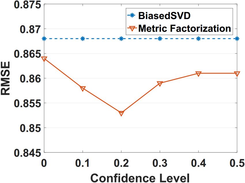
TABLE 1: Notations and Denotations                               user similarity computed by Jaccard similarity (s) from the
   Notations                             Descriptions
                                                                                interaction matrix. Assuming that we have three users: u1 ,
                                                                                u2 and u3 , the similarities based on interaction matrix are:
  R, M , N        Rating/interaction matrix, number of users and items.         s23 > s12 > s13 , then the corresponding user latent factors
      Y ,Ŷ       Distance matrix and predicted distance matrix.
   P , Q, k       User/item positions and its dimensionality.
                                                                                P1 , P2 and P3 can be positioned like Figure 1 (middle).
 bu , bi , µ, τ   User, item and global biases. scale factor for global bias.   Suppose we have another user u4 , and s41 > s43 > s42 ,
    cui , α       Confidence Value and its Confidence level.                    in this case, if we make P4 and P1 similar, the constraint
      a, b,       Distance scale factors.                                       s43 > s42 will not be satisfied no matter how we define P4
    l, λ, η       clip value, biases regularization rate, learning rate.
                                                                                in the same space. However, if we treat users as points in the
                                                                                same space, and make similar users closer to each other (that
3.1. Problem Formulation                                                        is, to make D23 < D12 < D13 , and D41 < D43 < D42 , D
                                                                                denotes distance), we can easily satisfy the aforementioned
    Suppose we have M users and N items, the rat-                               two constraints.
ing/interaction matrix is represented by R ∈ RM ×N . Let
u and i denote user and item respectively. Rui indicates the
preference of user u to item i. In most cases, most of the
entries in R are unknown, and the aim of recommender
system is to predict preference scores for these unseen
entries. The value of the R can be explicit ratings such as
rating score with range [1-5] or implicit feedback. Explicit
ratings can be utilized for rating estimation for unknown
entries, while implicit feedback can be used for generating                     Figure 1: An example for explaining the disadvantages of
personalized ranked recommendation lists (also known as                         Dot Product; Left: interaction matrix; Middle: user latent
one-class recommendations or top-n recommendation [17]).                        factors; Right: positions and distances with metric factor-
Implicit feedback such as view history, browsing log, click                     ization. All in 2-D dimension.
count and purchasing record are more abundant and easier
to acquire than explicit feedback, but explicit ratings still
play a critical role in modern recommender systems. In this                     4. Introduction to Metric Factorization
work, we will investigate both of them and explore/evaluate                         To tackle the disadvantage of matrix factorization and
them individually. Here, the definition of implicit feedback                    tap into the power of positions and distance, we propose a
is as follows:                                                                  novel recommendation model namely, metric factorization.
                 (
                    1, if interaction < u, i > exists                           Unlike matrix factorization which treats users and items as
          Rui =                                           (1)                   vectors in a new space, metric factorization considers the
                    0, otherwise
                                                                                users and items as points in a low-dimensional coordinate
The interaction can flexibly represent any kind of implicit                     system and their relationships are represented by Euclidean
feedback. 1 indicates that the user item pair (u, i) is ob-                     distances. As its name indicates, metric factorization factor-
served. 0 does not necessarily mean the user dislikes the                       izes the distance between users and items to their positions.
item, it can also indicate the user does not realize the                            Matrix factorization learns user and item latent factors
existence of item i. We treat items i as a positive sample                      via factorizing the interaction matrix which indicates the
for user u if Rui = 1, and as a negative sample if Rui = 0.                     similarities between users and items. Nonetheless, to learn
    For a clear presentation, Table 1 summarizes the nota-                      the user and item positions, we cannot directly utilize the
tions and denotations used in this paper.                                       rating/interaction matrix R since distance and similarity are
                                                                                two opposite concepts. Thus, we need to firstly convert the
3.2. Limitation of Matrix Factorization                                         R into distance matrix Y . To this end, we adopt a simple
                                                                                but effective principle:
    Leaving aside the success of matrix factorization for                         Distance(u, i) = Max Similarity − Similarity(u, i) (2)
recommendation tasks, it is not without flaws. One major
problem is that dot product restricts the expressiveness                        With this equation, highest similarity will become zero
of matrix factorization [18]. Dot product cares about the                       which indicates that the distance between u and i is zero.
magnitudes and angles of two vectors. To some extent, it                        Through this flip operation, we manage to convert similarity
measures the similarities rather than distances of the two                      to distance while keeping its distribution properties. This
vectors in terms of both magnitude and angle3 . Here we                         conversion can be applied to both explicit rating scores
extend an example from [18]. As shown in Figure 1, we                           or binary interaction data by just defining the maximum
attempt to use the user latent factors (P1 , P2 , P3 , P4 ) to                  similarity based on the range of feedback. We will specify
model the similarities of users and compare it with the                         it in the following sections.
                                                                                     Distance (or Metric, in mathematics, distances and met-
  3. In fact, dot product boils down to cosine similarity when ignoring the     rics are synonyms, so we will use these two words inter-
magnitude                                                                       changeably) is a numerical measurement of how far apart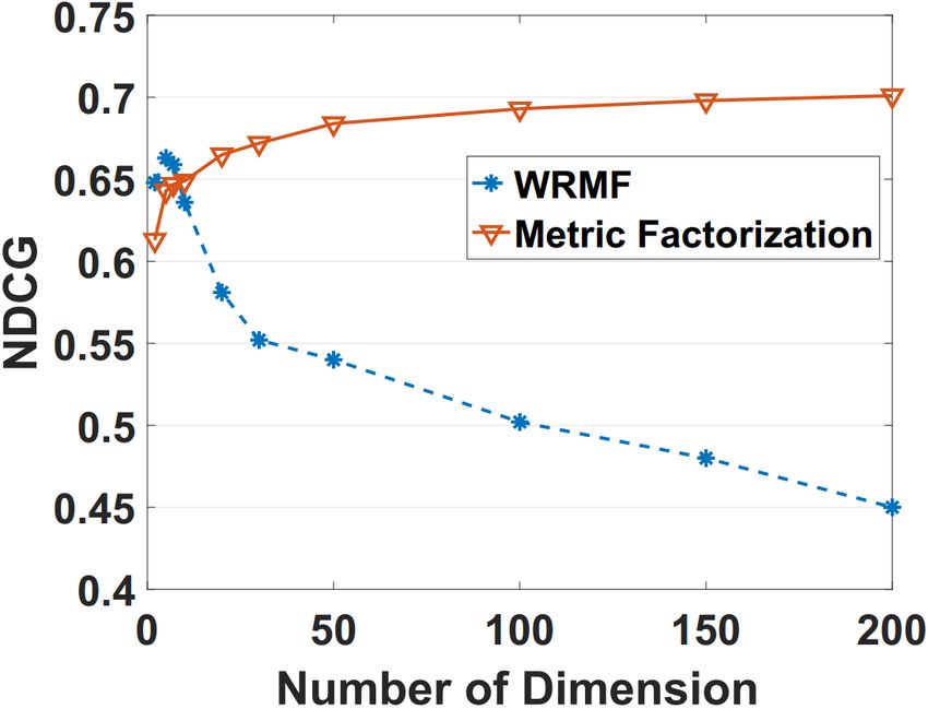
Figure 2: A simplified illustration of Metric Factorization. It mainly has two steps: First, convert similarity matrix (rating
matrix or interaction matrix) to distance matrix via equation 2. Second, factorize the distance matrix into user and item
positions in a low-dimensional space. In the last graph, solid line represents known distances and dash line indicates
unknown distances. Once the positions of users & items are learned, unknown distances can be easily derived for making
recommendation.

objects are. Distance function should satisfy four critical      factorize a big and sparse matrix into two more manage-
conditions: non-negativity, identity of indiscernibles, sym-     able, compact matrices, this factorization operation and the
metry and triangle inequality. There are many metrics that       learned matrices have totally different physical interpreta-
are used in different application domains or scenarios such      tions. Nonetheless, we can associate the Pu and Qi of metric
as discrete metric, Euclidean metric, Graph metric, etc.         factorization with user’s preferences and item latent features
In the Euclidean space Rk , distance between two points          in the same way as matrix factorization.
are usually measured by Euclidean distance (or `2 -norm              Figure 2 simply illustrates the procedure of metric fac-
distance). That is:                                              torization (for rating prediction). First, we get the distance
                                   k
                                                 !1/2            matrix from the similarity matrix with Equation 2, then we
                                  X
                                               2                 factorize the distance matrix and learn the positions of users
         D(u, i) =k u − i k2 =       |ui − ii |           (3)
                                                                 and items. After attaining the positions, if required, we can
                                   i=1
                                                                 easily recover every entry of the similarity matrix and make
Euclidean distance has been widely used in machine learn-        recommendations.
ing, sensor networks, geometry, etc., due to its simple form
and useful properties [19]. In practice, squared distance is
usually adopted to avoid the trouble of computing the square
                                                                 5. Metric Factorization for Rating Prediction
root.
    In metric factorization, we will utilize the Euclidean           As aforementioned, metric factorization can be applied
distance to measure the distance between users and items         to both rating prediction and item ranking. In this section,
in a low-dimensional coordinate system. Let k denote the         we will introduce how to perform rating prediction with
dimensionality of the space. For each user and item, we          metric factorization.
assign a vector: Pu ∈ Rk and Qi ∈ Rk , to determine
its position in this multidimensional space. After that, we      5.1. Basic Model
measure the distance between user and item with Euclidean
Distance:                                                            For rating prediction, it is enough and more efficient to
                   D(u, i) =k Pu − Qi k22                 (4)    just consider observed interaction data. Let K denote the set
                                                                 of observed rating data.
In real-world recommender applications, only some entries
of the distance matrix are known. The goal of metric fac-            First, we convert the rating matrix R into distance met-
torization is to learn the user and item positions given the     rics with the following equation:
partially observed distance matrix:                                                  Yui = Rmax − Rui                       (6)
                        f (Pu , Qi |Y )                   (5)
                                                                 Where Rmax is the possible maximum rating score. Note
The function f varies with the task of recommendation            that we use explicit ratings here, thus, if Rmax = 5, the
(rating prediction and item ranking). We will detail the         rating score of 3, then the distance Yui = 5 − 3 = 2.
formulation with regard to different tasks in the following          Afterwards, we need to choose a loss function. Tradi-
sections.                                                        tional pairwise loss used in metric learning is not suitable
    So far, we are aware that matrix factorization and metric    for rating prediction as we need to recover the precise rating
factorization are very much alike. Although both of them         value instead of a ranked list. Therefore, we adopt the widely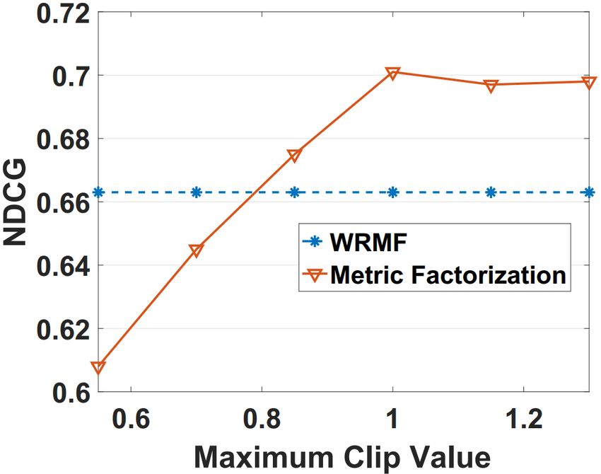
used squared loss and we learn the user and item positions       5.3. Regularization
by minimizing the following loss:
                      X                                             Training on the observed ratings can easily lead to
         L(P, Q) =        (Yui − k Pu − Qi k22 )2      (7)
                                                                 overfitting. Traditional matrix factorization usually adopt `2 -
                       (u,i)∈K
                                                                 norm regularization on latent factors and biases to avoid
This model is closely related to basic matrix factorization,     over-complex solutions. For the user and item biases, we
the only difference is that we replace the dot product with      apply the widely used `2 norm same as [9].
Euclidean distance.
                                                                 5.3.1. Norm Clipping. For P and Q, `2 norm regularization
5.2. Adding Biases and Confidences                               is undesirable as it will push users and items close to the
                                                                 origin. Instead of minimizing the `2 regularization, we relax
5.2.1. Adding Biases. The above basic model only con-            the constraints to the Euclidean ball and perform `2 norm
siders the user and item interactions. However, individual       clipping after each updates.
effects of users or items also matter. For example, some
items tend to receive higher ratings; some users tend to give                       k Pu k2 ≤ l, k Qi k2 ≤ l                (11)
low rating scores. Same as biased matrix factorization [9],
we also introduce the global, user and item bias terms to        Where l control the size of the Euclidean ball. These two
metric factorization. Thus, the distance between user and        constraints work as regularization to restrict the value of
item is formulated as follows:                                   Uu and Vi in `2 -norm unit ball so that the data points will
                                                                 not spread too widely [14], [22]. This operation is generally
                 Ŷ =k Pu − Qi k22 +bu + bi + µ            (8)   performed when updating the parameters in every iteration.
Here, Ŷ denotes the predicted distances. bu is the bias term
of user u; bi is the bias term of item i; µ is the global bias   5.3.2. Dropout. Dropout is a simple but useful approach
which equals to the mean distance constructed from training      for tackling overfitting problem in neural networks [23].
data. Usually, we can add a hyper parameter τ to scale µ         The main idea is to drop some neurons during training
as the mean distance cannot always reflect the real global       stage to avoid co-adaptation between neural units. Here,
bias.                                                            we propose a similar method and apply it to metric fac-
                                                                 torization. As Equation (3) indicated, the final distance is
5.2.2. Confidence Mechanism. Another important aspect            the addition of the distance of each dimension. To prevent
we would like to consider is the reliability and stability of    the co-adaptations among dimensions, we propose randomly
the rating data. Most rating prediction algorithms ignore the    dropping the some dimensions and computing the overall
noise of ratings and assume that all ratings can be treated as   distance with the remaining dimensions.
ground truth. Nonetheless, not all observed ratings deserve
the same weight [9]. For example, some users might give                    k Pu − Qi k22 = |Pu1 − Qi1 |2 + |Pu2 − Qi2 |2 +
                                                                                                           |    {z     }
two different scores when being asked to rate the same                                                             drop
item twice at different time [20]. Former studies [20], [21]       |Pu3 − Qi3 |2 +... + |Puj − Qij |2 + ... + |Puk − Qik |2
suggest that extreme ratings (e.g., 1 and 5) are more reliable     |    {z     }                              |    {z     }
                                                                         drop                                        drop
than moderate ratings (e.g, 2, 3 and 4). To alleviate this
issue, we propose adding a confidence value cui for each         In the above example, we remove the second, third and k th
rating score and revise the loss function to:                    dimension, so these dimensions will not contribute to the
                                                                 distance prediction in that epoch. The dropped dimensions
         X
  L=           cui (Yui − (k Pu − Qi k22 +bu + bi + µ)) (9)
       (u,i)∈K
                                                                 are subject to change in each epoch. Note that this dropout
                                                                 operation is only carried out during the training period.
Note that the confidence cui can represent many factors such
as reliability, implicit feedback by specifying the confidence
definition. Inspired by the conclusion of [20], we design        6. Metric Factorization for Item Ranking
a novel confidence mechanism to assign higher confidence
values to more reliable ratings.                                     Item ranking is another important task of recommender
                                             max                 systems where only implicit feedback is available. Explicit
                                         R
                 cui = 1 + α · g(Rui −        )          (10)    ratings are not always present in many real-world applica-
                                          2                      tions, nonetheless, there is often nontrivial information about
Where g(·) can be absolute, square, or even logarithm            the interactions, such as purchase records, listen to tracks,
functions. α (confidence level) is a hyper-parameter to          clicks, and even rating itself can also be viewed as a kind
control the magnitude of the confidence. This confidence         of implicit feedback [24], [25]. In reality, the amount of
mechanism ensures extreme ratings to get higher confidence.      implicit data of some applications far outweighs the quantity
It is flexible to replace this confidence strategy with other    of explicit feedback, this makes implicit feedback to be the
advanced ones.                                                   primary focus in some systems.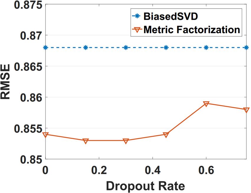
observation, for example, if a user browses the item twice,
                                                                 then wui = 2. For large numbers, we can also convert it to
                                                                 log-scale like [3]. Since this information is usually absent
                                                                 in publicly available dataset, we set w to Rui (0 or 1).
                                                                 The functionality of hyper-parameter α is the same as that
                                                                 Equation 10. For regularization, we take the same approach
                                                                 including `2 -norm clipping and dropout as described in
                                                                 Section 5.3.
                                                                      Figure 3 illustrates an example of how the proposed
                                                                 approach works. Our model can not only force users and
                                                                 their preferred items closer but also push unpreferred items
                                                                 away even though we adopt a pointwise training scheme.
Figure 3: Illustration of the proposed approach. Here we give    Unlike most metric learning based models, which enforce
an example which consists of three users and their preferred     imposters outside of the user territory by some finite mar-
items. The original positions are randomly initialized. After    gin, the confidence mechanism in this approach provides
training, items that user likes will surround her within a       possibility for negative items to invade user territory, which
finite distance.                                                 is beneficial for recommendation task as it can work as a
                                                                 filter to select negative items for recommendation. Another
                                                                 important characteristic of our model is that it can indirectly
    First, we need to convert the similarity into distance.      cluster users who share a large amount of items together.
Following the principle (2), we conduct the transformation       This property makes it possible to capture the relationships
with the following equation:                                     between neighbourhoods which are also important for item
                                                                 recommendation [26].
               Yui = a · (1 − Rui ) + z · Rui            (12)
Since Rui equals either 0 or 1, the distance Yui = a if          7. Learning of Metric Factorization
Rui = 0 and Yui = z if Rui = 1. These two hyper-
parameters make it very flexible to control the user and item    7.1. Optimization and Recommendation
distances. When setting the value of a and z , we need to
ensure the inequality: a > z , to make the distance between          We optimize the both the rating estimation and ranking
user and uninteracted item greater than that between user        learning model with Adagrad [27]. Adagrad adapts the step
and interacted item. Usually, we can set z to zero. As Rui       size to the parameters based on the frequencies of updates.
equals either “1” or “0”, all < user, positive item > (or        Thus, it reduces the demand to tune the learning rate. The
< user, negative item >) has same distance unlike rating         learning process for metric factorization is shown below.
prediction whose distances vary with the rating scores.
    For ranking task, it is usually beneficial to take the       Procedure 1 Training Procedure of Metric Factorization
unobserved interactions (negative sample) into considera-        Input: R, k , P , Q, learning rate η , α, l, a and z , (bu , bi ,
tion. Such as Bayesian personalized ranking, Collaborative           τ , λ)
metric learning, or weighted matrix factorization [3], neural     1: procedure I NITIALIZATION
collaborative filtering [5], the former two models are trained    2:      initialize P , Q, (and bu , bi ) with normal distribution.
in pairwise manner which sample a negative item for each          3: end procedure
observed interaction. WRMF adopts a pointwise learning            4: procedure M ODEL L EARNING
approach but also considers negative items. To learn the          5:      for all pairs (u, i) in current batch do
positions of users and items from implicit data, we employ        6:           update Pu and Qi (and bu , bi ) with Adagrad
a pointwise approach and minimize the following weighted          7:           clip Pu and Qi by `2 -norm with l
square loss.                                                      8:      end for
                                                                  9: end procedure
                       X
        L(P, Q) =             cui (Yui − k Pu − Qi k22 )2
                                                                 Output: P ,Q, (and bu , bi )
                    (u,i)∈R
                         s.t. k Pu k2 ≤ l, k Qi k2 ≤ l
                                                                     During the testing, we can compute the distance between
It is similar to equation (7). The major difference is that      target user and item positions. As for rating prediction, we
we consider all unobserved interactions and bias terms are       reconstruct the ratings using the following rule:
removed. cui is also a confidence value, here, it is adopted
to model the implicit feedback and is defined as:                                      R̂ui = Rmax − Ŷui                      (14)

                      cui = 1 + αwui                     (13)    For example, if the predicted distance is Ŷui = 4 and
                                                                 Rmax = 5, then the predicted rating score is 1. For item
Where wui represents the observation of implicit feedback,       ranking, we directly rank the predicted distance in descend-
we can simply treat the counts of implicit actions as the        ing order instead of ascending order as we usually do in
matrix factorization. Smaller distance indicates that the user    TABLE 2: Number of users, items, ratings and correspond-
is more likely to be interested in the item. Therefore we will    ing density of four adopted datasets for rating prediction.
recommend users with items that close to them.                           Datasets           #Items   #Users   #Ratings   Density
                                                                         Goodbooks          10K      53K        6M       1.119%
7.2. Model Complexity                                                    Movielens Latest   9.1K     0.7K      100K      1.644%
                                                                         Movielens 100K     1.7K     0.9K      100k      6.305%
    The computation for rating prediction is linear to the               Movielens 1M       3.7K      6K        1M       4.468%
number of ratings and it can be trained in O(|K|k), where
k is the dimension of latent factors and |K| is the number of
                                                                  8.1.2. Evaluation Metrics. We employ two widely used
ratings. For item ranking, since all entries of the interaction
                                                                  metrics: Root Mean Squared Error (RMSE) and Mean Aver-
matrix are involved, the model complexity is O(|R|k). As
                                                                  age Error (MAE), to assess prediction errors. MAE measures
for the computation time (on GPU), it takes about 50s to get
                                                                  the average magnitude of the errors in a set of predictions,
satisfactory recommendation performance for rating estima-
                                                                  while RMSE tends to disproportionately penalize large er-
tion on Movielens 100K. For item ranking, the computation
                                                                  rors [28]. Since these metrics are commonplace for rec-
time for each epoch is about 15s, and it usually takes less
                                                                  ommendation evaluation, we omit the details of evaluation
than 30 epochs to achieve a satisfactory result.
                                                                  metrics for brevity.
8. Experiments
                                                                  8.1.3. Baselines. We compare our approach with the fol-
    In this section, we describe the evaluation settings and      lowing baselines.
show the performance of metric factorization. As rating
prediction and item ranking are usually investigated sep-            •      Average. This approach predicts ratings based on
arately with different evaluation metrics, we evaluate the                  average historical ratings and has two variants: User-
metric factorization based rating prediction and item rank-                 Average and ItemAverage.
ing models individually. We implement metric factorization           •      SlopOne [29]. It is an efficient online rating-based
with Tensorflow4 and conduct experiments on a NVIDIA                        collaborative filtering approach.
TITAN X Pascal GPU. We empirically evaluate the proposed             •      BPMF [10]. This model considers the matrix factor-
methodology mainly to answer the following three research                   ization from a probabilistic perspective and provides
questions:                                                                  a fully Bayesian treatment by solving it with Markov
    •   RQ1 Does the proposed methodology make more                         chain Monte Carlo.
        accurate rating estimation than MF and neural net-           •      BiasedSVD. This model introduces the bias to both
        work based models?                                                  user and items and equips basic matrix factorization
    •   RQ2 Can the proposed approach outperform neural                     to model the user/item specific characteristics.
        network and metric learning approaches in terms of           •      NRR [30]. NRR is a neural rating regression model
        item ranking?                                                       which captures the user and item interactive rela-
    •   RQ3 How do the hyper-parameters impact the model                    tionships with neural network regression.
        performances?                                                •      NNMF [31]. This model replaces the simple dot
                                                                            product of matrix factorization with multi-layered
8.1. Evaluation for Rating Prediction                                       neural network and decomposes it into two latent
                                                                            vectors for both users and items.
8.1.1. Datasets Descriptions. We evaluate the effectiveness
of our approach on rating prediction using the following
datasets:                                                         8.1.4. Experimental Setups. We optimize our model in
    •   Goodbooks. This dataset contains six million ratings      mini batch mode. For a fair comparison, we randomly split
        for about ten thousand most popular books. It is          each dataset into a training set and a test set by the ratio
        collected from a real-word book website5 .                of 9:1, and report the average results over five different
    •   Movielens Datasets. We use three versions of pub-         splits. Hyper-parameters for compared baselines are care-
        licly available Movielens data including Movielens        fully tuned to achieve their best performances. Our model
        100K,Movielens 1M and Movielens Latest. Movie-            is not very sensitive to small variations of learning rate. This
        lens 100K and Movielens 1M are widely adopted             is mainly due to the adaptive gradient optimizer we adopted
        benchmark movie data collected by GroupLens re-           as it can eliminate the demand to tune the learning rate.
        search Project. Movielens Latest is a comparatively       Thus, we set the learning rate to 0.05 for all datasets. The
        new dataset which includes historical interactions        bias regularization rate λ is set to 0.01 excerpt for Movielens
        between 1995 to the year 2016.                            latest (λ = 0.05). The confidence level α is set to 0.2 excerpt
                                                                  for Movielens 1M (α = 0.1). g(·) is set to square function
Table 2 summarizes the statistics of these four datasets.         for Goodbooks, Movielens latest and 1M and it is set to
  4. https://tensorflow.org                                       absolute function for Movielens 100k. Other parameters are
  5. http://fastml.com/goodbooks-10k                              listed as follows:
TABLE 3: Comparison between our approach and baselines in terms of RMSE and MAE.
Best performance is in boldface and second best is underlined.

                                  Datasets      Goodbooks               Movielens Latest       Movielens 100K       Movielens 1M
                                   Models                                   Root Mean Squared Error
                              UserAverage     0.893 ± 0.001              0.967 ± 0.005          1.047 ± 0.004      1.036 ± 0.002
                              ItemAverage     0.953 ± 0.002              0.991 ± 0.008          1.035 ± 0.005      0.978 ± 0.001
                                SlopOne       0.825 ± 0.001              0.907 ± 0.007          0.935 ± 0.001      0.899 ± 0.002
                                 BPMF         0.829 ± 0.001              0.932 ± 0.001          0.927 ± 0.003      0.867 ± 0.002
                               BiasedSVD      0.846 ± 0.001              0.868 ± 0.005          0.911 ± 0.003      0.847 ± 0.002
                                  NRR         0.822 ± 0.001              0.876 ± 0.002          0.909 ± 0.003      0.875 ± 0.002
                                 NNMF         0.821 ± 0.001              0.871 ± 0.006          0.903 ± 0.002      0.843 ± 0.002
                                MetricF       0.803 ± 0.001              0.853 ± 0.006          0.891 ± 0.005      0.836 ± 0.001
                                   Models                                      Mean Average Error
                              UserAverage     0.700 ± 0.001              0.753 ± 0.002          0.839 ± 0.004      0.830 ± 0.002
                              ItemAverage     0.762 ± 0.002              0.769 ± 0.004          0.825 ± 0.005      0.782 ± 0.001
                                SlopOne       0.638 ± 0.001              0.693 ± 0.007          0.737 ± 0.001      0.710 ± 0.002
                                 BPMF         0.639 ± 0.001              0.707 ± 0.001          0.725 ± 0.003      0.678 ± 0.001
                               BiasedSVD      0.668 ± 0.001              0.666 ± 0.002          0.718 ± 0.002      0.665 ± 0.003
                                  NRR         0.631 ± 0.003              0.674 ± 0.005          0.717 ± 0.005      0.691 ± 0.002
                                 NNMF         0.637 ± 0.001              0.667 ± 0.004          0.709 ± 0.002      0.669 ± 0.001
                                MetricF       0.616 ± 0.001              0.656 ± 0.004          0.696 ± 0.005      0.654 ± 0.001

TABLE 4: Hyper-parameter settings for rating prediction.                                 TABLE 5: Statistics of datasets used for item ranking.
 Dataset                             Hyper-parameters                                          Datasets         #Items   #Users    #Interact   %Density
 Goodbooks           k   = 200,   dropout = 0.10,   τ   = 0.80,   l   = 1.00                   YahooMovie       11.9K     7.6K     221.4K      0.243%
 Movielens Latest    k   = 250,   dropout = 0.15,   τ   = 0.80,   l   = 0.85                   YahooMusic        1.0K    15.4K     365.7K      2.374%
 Movielens 100k      k   = 150,   dropout = 0.05,   τ   = 0.90,   l   = 1.00                   FilmTrust         2.1K     1.5K      35.5K      1.137%
 Movielens 1M        k   = 150,   dropout = 0.03,   τ   = 0.50,   l   = 1.40                   EachMovie        61.3K     1.6K     2.811M      2.369%

8.1.5. Results and Discussions. From Table 3, we observed                                  •     FilmTrust. FilmTrust is crawled from a film sharing
that our model consistently outperforms all compared meth-                                       and rating website by Guo et al. [32]. In this work,
ods including classic matrix factorization based models as                                       we do not use the trust information in this dataset.
well as neural network based models on all datasets. Specif-                               •     EachMovie. EachMovie7 is also a movie dataset
ically, Metric factorization achieves substantial improve-                                       which is widely adopted for recommendation eval-
ments over BPMF and BiasedSVD. Naive approaches User-                                            uation.
Average and ItemAverage perform poorly on all datasets.
Recent neural network based model NRR and NNMF are                                      Table 5 summarizes the details of the datasets. All of
two competitive baselines especially on large scale dataset                         the interactions are binarized by the method introduced in
Goodbooks. However, NRR does not perform well on other                              Section 3.1.
three datasets. With this table, we can give a sure answer to
RQ1.                                                                                8.2.2. Evaluation Metrics. To evaluate the ranking accu-
                                                                                    racy and quality, we employed five widely used metrics:
8.2. Evaluation for Item Ranking                                                    Recall, Precision, Mean Average Precision (MAP), Mean
                                                                                    Reciprocal Rank (MRR) and Normalized Discounted Cu-
    In this section, we evaluate the performance of metric                          mulative Gain (DNCG). In most cases, users only care
factorization on item ranking tasks.                                                about the topmost recommended items, so we employ these
                                                                                    evaluations at a given cut-off n and denote them as: Pre-
8.2.1. Datasets Description. We also report the experimen-                          cision@n and Recall@n. In practice, making items that
tal results over four real-world datasets. The datasets are                         interest target users more rank higher will enhance the
described as follows:                                                               quality of recommendation lists. MAP, MRR and NDCG are
                                                                                    three rank-aware measurements with which higher ranked
    •      Yahoo Research Dataset. It consists of two
                                                                                    positive items are prioritized. Thus they are suitable for
           datasets: Yahoo movie and Yahoo music. Both of
                                                                                    assessing the quality of ranked lists [33]. MRR cares about
           them are provided by Yahoo Research Alliance Web-
                                                                                    the single highest-ranked relevant item. NDCG is deter-
           scope program6 . The music preference dataset is
                                                                                    mined by Discounted Cumulative Gain and Ideal Discounted
           collected from Yahoo Music services.
  6. http://research.yahoo.com/Academic Relations                                     7. http://www.cs.cmu.edu/ lebanon/IR-lab/data.html
TABLE 6: Performance comparison on item ranking task in terms of MAP, MRR, NDCG, Precision and Recall on four
datasets. Best performance is in boldface and second best is underlined.
Methods MAP MRR NDCG P@5 P@10 R@5 R@10
YahooMovie
POP 0.160 ± 0.001 0.323 ± 0.002 0.386 ± 0.002 0.128 ± 0.001 0.097 ± 0.002 0.160 ± 0.003 0.239 ± 0.002
ItemKNN 0.177 ± 0.001 0.338 ± 0.002 0.395 ± 0.001 0.155 ± 0.003 0.122 ± 0.002 0.180 ± 0.001 0.275 ± 0.002
BPR 0.161 ± 0.001 0.322 ± 0.001 0.387 ± 0.001 0.128 ± 0.001 0.096 ± 0.002 0.161 ± 0.001 0.240 ± 0.001
NeuMF 0.171 ± 0.001 0.329 ± 0.006 0.402 ± 0.004 0.140 ± 0.002 0.112 ± 0.001 0.168 ± 0.002 0.256 ± 0.003
WRMF 0.209 ± 0.001 0.384 ± 0.002 0.435 ± 0.004 0.176 ± 0.001 0.135 ± 0.001 0.209 ± 0.001 0.310 ± 0.001
CDAE 0.224 ± 0.002 0.409 ± 0.005 0.453 ± 0.003 0.188 ± 0.003 0.143 ± 0.002 0.226 ± 0.003 0.331 ± 0.004
CML-PAIR 0.223 ± 0.002 0.416 ± 0.003 0.456 ± 0.003 0.189 ± 0.004 0.147 ± 0.002 0.224 ± 0.003 0.332 ± 0.002
CML-WARP 0.235 ± 0.002 0.440 ± 0.005 0.466 ± 0.001 0.202 ± 0.001 0.153 ± 0.001 0.237 ± 0.002 0.342 ± 0.002
MetricF 0.262 ± 0.001 0.466 ± 0.002 0.486 ± 0.001 0.222 ± 0.001 0.167 ± 0.001 0.262 ± 0.002 0.374 ± 0.002
YahooMusic
POP 0.100 ± 0.001 0.237 ± 0.003 0.334 ± 0.001 0.088 ± 0.001 0.072 ± 0.002 0.103 ± 0.002 0.166 ± 0.002
ItemKNN 0.132 ± 0.002 0.299 ± 0.001 0.375 ± 0.002 0.115 ± 0.002 0.090 ± 0.002 0.135 ± 0.003 0.207 ± 0.001
BPR 0.133 ± 0.001 0.300 ± 0.002 0.373 ± 0.001 0.118 ± 0.001 0.092 ± 0.001 0.141 ± 0.002 0.215 ± 0.001
NeuMF 0.141 ± 0.002 0.319 ± 0.005 0.383 ± 0.003 0.130 ± 0.002 0.099 ± 0.001 0.155 ± 0.001 0.232 ± 0.003
WRMF 0.144 ± 0.001 0.333 ± 0.003 0.386 ± 0.001 0.130 ± 0.002 0.097 ± 0.001 0.153 ± 0.002 0.226 ± 0.002
CDAE 0.153 ± 0.003 0.348 ± 0.006 0.395 ± 0.004 0.136 ± 0.002 0.102 ± 0.001 0.163 ± 0.002 0.240 ± 0.003
CML-PAIR 0.148 ± 0.002 0.339 ± 0.003 0.390 ± 0.003 0.134 ± 0.003 0.102 ± 0.002 0.159 ± 0.002 0.236 ± 0.004
CML-WARP 0.153 ± 0.002 0.353 ± 0.005 0.393 ± 0.002 0.140 ± 0.002 0.103 ± 0.001 0.171 ± 0.002 0.249 ± 0.003
MetricF 0.169 ± 0.001 0.375 ± 0.002 0.411 ± 0.001 0.152 ± 0.001 0.114 ± 0.001 0.183 ± 0.001 0.268 ± 0.002
EachMovie
POP 0.259 ± 0.001 0.457 ± 0.001 0.522 ± 0.001 0.227 ± 0.001 0.172 ± 0.002 0.203 ± 0.001 0.267 ± 0.002
ItemKNN 0.407 ± 0.001 0.636 ± 0.002 0.649 ± 0.001 0.364 ± 0.002 0.291 ± 0.001 0.333 ± 0.002 0.469 ± 0.003
BPR 0.394 ± 0.003 0.627 ± 0.002 0.641 ± 0.002 0.346 ± 0.001 0.293 ± 0.001 0.313 ± 0.001 0.448 ± 0.001
NeuMF 0.414 ± 0.003 0.656 ± 0.002 0.657 ± 0.003 0.378 ± 0.003 0.302 ± 0.002 0.335 ± 0.003 0.475 ± 0.001
WRMF 0.433 ± 0.001 0.679 ± 0.001 0.670 ± 0.002 0.397 ± 0.002 0.314 ± 0.001 0.355 ± 0.002 0.494 ± 0.001
CDAE 0.432 ± 0.003 0.678 ± 0.003 0.673 ± 0.002 0.394 ± 0.004 0.311 ± 0.003 0.356 ± 0.003 0.497 ± 0.002
CML-PAIR 0.426 ± 0.003 0.674 ± 0.002 0.668 ± 0.001 0.399 ± 0.001 0.315 ± 0.002 0.348 ± 0.002 0.492 ± 0.001
CML-WARP 0.419 ± 0.001 0.683 ± 0.001 0.663 ± 0.002 0.398 ± 0.001 0.312 ± 0.001 0.346 ± 0.002 0.485 ± 0.003
MetricF 0.454 ± 0.001 0.696 ± 0.002 0.687 ± 0.001 0.416 ± 0.001 0.330 ± 0.001 0.370 ± 0.002 0.515 ± 0.002
FilmTrust
POP 0.489 ± 0.002 0.618 ± 0.004 0.650 ± 0.002 0.418 ± 0.004 0.350 ± 0.002 0.397 ± 0.008 0.631 ± 0.004
ItemKNN 0.222 ± 0.009 0.362 ± 0.037 0.331 ± 0.006 0.196 ± 0.004 0.180 ± 0.004 0.218 ± 0.004 0.351 ± 0.002
BPR 0.476 ± 0.004 0.600 ± 0.007 0.635 ± 0.003 0.412 ± 0.005 0.347 ± 0.001 0.391 ± 0.009 0.613 ± 0.007
NeuMF 0.483 ± 0.001 0.609 ± 0.005 0.646 ± 0.003 0.413 ± 0.003 0.350 ± 0.002 0.393 ± 0.004 0.626 ± 0.007
WRMF 0.516 ± 0.002 0.648 ± 0.005 0.663 ± 0.002 0.433 ± 0.002 0.351 ± 0.001 0.427 ± 0.005 0.632 ± 0.007
CDAE 0.523 ± 0.008 0.654 ± 0.010 0.678 ± 0.008 0.436 ± 0.004 0.353 ± 0.003 0.441 ± 0.006 0.647 ± 0.005
CML-PAIR 0.491 ± 0.002 0.637 ± 0.003 0.655 ± 0.001 0.418 ± 0.002 0.337 ± 0.001 0.408 ± 0.003 0.602 ± 0.003
CML-WARP 0.529 ± 0.004 0.666 ± 0.005 0.684 ± 0.003 0.438 ± 0.005 0.359 ± 0.003 0.441 ± 0.007 0.653 ± 0.004
MetricF 0.549 ± 0.005 0.685 ± 0.006 0.701 ± 0.004 0.453 ± 0.003 0.366 ± 0.002 0.462 ± 0.006 0.672 ± 0.006
Cumulative Gain. Detail definitions are omitted for the sake BPR optimization criterion aims to maximize the
of conciseness. differences between negative and positive samples.
• WRMF [3]. It is an effective ranking model for
8.2.3. Baselines. We compare our model with the following implicit feedback. It uses dot product to model the
classic and recent strong baselines: user item interaction patterns as well.
• NeuMF [18]. NeuMF combines multi-layered pre-
• POP. It is a non-personalized method which gener- ceptron with generalized matrix factorization and
ates recommendations according to the item popu- computes the ranking scores with a neural layer
larity and recommends users with the most popular instead of dot product. It treats the ranking problem
items. as a classification task and optimizes the model by
• ItemKNN [34]. Item-based collaborative filtering minimizing the cross entropy loss.
method recommends items which are similar to • CDAE [13]. CDAE learns user and item distributed
items the user has liked. Here the similarity between representations from interaction matrix with autoen-
items is computed with cosine function. coder. Denoising technique is utilized to improve
• BPR [2]. It is a generic pairwise optimization crite- generalization and prevent overfitting. Here, we use
rion and works even better by integrating MF. The logistic loss to optimize the network as it is reportedto achieve the best performances in the original more plausible to model user item interaction patterns than
paper. other forms. Third, neural network based models CDAE and
• CML [14]. CML is competitive baseline for the NeuMF are strong baselines and outperform traditional ma-
proposed approach. Here, we train it with two trix factorization. Even though NeuMF and BPRMF adopt
types of loss: pairwise hinge loss and weighted negative sampling, NeuMF gets more accurate results than
approximate-rank pairwise loss (WAPR). Note that BPRMF. CDAE performs better than WRMF in most cases.
the WARP loss is computational intensive due to This suggests the certain effectiveness of introducing non-
the pre-computations for negative samples. Here, we linearity. However, there is still a huge performance gap
set the negative sampling number to 20 to avoid between these models and our approach, which also demon-
extended computing time. strates the superiority of metric factorization compared to
neural based approach.
BPR and WRMF are matrix factorization based models;
In words, these observations demonstrate the advan-
NeuMF and CDAE are neural network based models; CML-
tages of considering the recommendation problem from the
PAIR and CML-WARP are metric learning based models.
positions and distances perspective, and the experiments
8.2.4. Implementation Details. We adopt the implementa- empirically show the efficacy of the method we adopted
tion of Mymedialite8 for POP, ItemKNN, BPR and WRMF. to learn users’ and items’ positions. With these results, we
For NeuMF, we use their released source code9 . We im- can give a sure answer to research question RQ2.
plemented all other models with Tensorflow. We test our
model with five random splits by using 80% of the in- 8.3. Model Parameter Analysis
teraction data as training set and the remaining 20% as
test set and report the average results. Hyper-parameters In this section, we will investigate the impact of
are determined with grid search. The dimensions of user model parameters to answer RQ3. All the experiments
and item vectors in our approach and CML are tuned are performed on Movielens Latest (Rating Prediction) and
amongst {80, 100, 120, 150, 200}. Learning rate of the pro- FilmTrust (Item Ranking). Due to limited space, we only
posed model is set to 0.1. The margin of CML-pair and report the RMSE for rating prediction and NDCG for item
CML-WARP is amongst {0.5, 1.0, 1.5, 2.0}. For all datasets, ranking. Matrix factorization model BiasedSVD and WRMF
we consider the interaction as the observation of implicit act as the baselines.
feedback and set wui = Rui (Here, Rui is constructed
from the training set.). Same as rating prediction, we set
the learning rate to 0.05 for all datasets. The dimension
k is set to 100 for EachMovie and k = 200 for other
three datasets. We find that simply setting the distance scale
factor z to 0 is sufficient for the adopted four datasets.
Another distance scale factor a is set to: 2.25 for FilmTrust,
2.0 for YahooMovie and EachMovie, 0.5 for YahooMusic.
The confidence level α is set to 4 for FilmTrust and 1 for
other three datasets. Dropout does not influence the ranking (a). Rating Prediction (b). Item Ranking
performance much on these four datasets, so we do not use Figure 4: (a) RMSE with varying Number of Dimension (k );
dropout in the experiments. (b) NDCG with varying Number of Dimension (k ).
8.2.5. Results and Discussions. Results in terms of the
MAP, MRR, NDCG, Precion and Recall at cut-off five
and ten are shown in Table 6. In particular, three key 8.3.1. Number of Dimension k . Figure 4(a) shows the
observations can be drawn from the results: varying RMSE on rating prediction for Movielens Latest.
First, the proposed approach consistently achieves the We observe that our model outperforms BiasedSVD with
best performances on all datasets. The overall performance same dimension settings, and it takes smaller dimension
gaining over WRMF model is up to 20.8%. Although both for metric factorization to reach the best performance. The
CML and the proposed approach rely on distance mea- overfitting issue on rating prediction of both models is not
surement, our model still outperforms the CML by up to serious. Figure 4(b) shows the varying NDCG on item
8.7%, which indicates that our model can reflect the dis- ranking for FilmTrust. Clearly, WRMF is easy to overfit with
tance relationship among users and items more accurately. large number of dimensions. Best performance of WRMF
Second, Euclidean distance based models (Metric factoriza- is usually achieved with a comparatively small number,
tion and CML) outperform methods that use dot product, and then the performance will decrease rapidly (a similar
neural network models and neighbourhood based models; phenomenon is also observed on other datasets.), which
The improvement suggests that metric based models are greatly limits the flexibility and expressiveness of the rec-
ommendation model. This might be due to the weakness of
8. http://mymedialite.net/index.html dot product we explained in Section 3.2. While our model
9. https://github.com/hexiangnan/neural collaborative filtering is less likely to overfit with comparatively large number(a). Rating Prediction (b). Item Ranking (a). Rating Prediction (b). Item Ranking
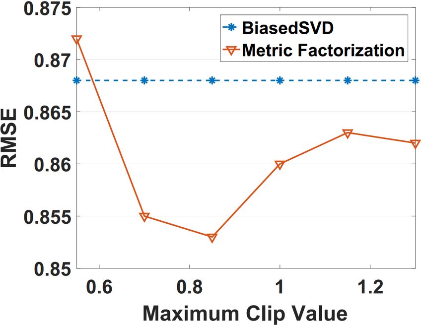
Figure 5: (a) RMSE with varying maximum clip value; (b) Figure 7: (a) RMSE with varying dropout rate; (b) NDCG
NDCG with varying maximum clip value. with varying distance scale factor a.
of dimensions, the performances are usually enhanced by
dropout does improve the performance of rating prediction.
increasing the dimension size properly, which allows the
Nonetheless, the dropout rate is usually set to a small value
model to capture more factors of user preferences and item
as we do not want to drop useful information. Unfortunately,
characteristics on personalized ranking task.
we find that the dropout operation does not favor the ranking
based model.
8.3.2. Maximum Clip Value l. Figure 5 shows the impacts
of maximum clip value l on model performance. l is a
8.3.5. Distance Scale Factor a. Since another distance
critical model parameters as it controls the scope of user
scale factor z is set to 0, we only analyze parameter a.
and item positions. Intuitively, ideal clip value might be
It controls the minimum distance that we would like to
determined by the range of feedback value (e.g., ratings,
push the negative items away from the users. As shown
binary implicit feedback). Since the implicit feedback in our
the Figure 7(a), a does not have as much influence as other
work is set to 0 or 1, setting l to 1 is enough in most cases.
parameters like k and l. The performance on FilmTrust does
While for rating prediction, the rating score range could be
not fluctuate much with a being set to 1.75 - 2.5.
diverse, so l should be carefully tuned.
9. Conclusion and Future Work
In this paper, we propose the metric factorization which
treats the recommendation problem from a novel perspec-
tive. Instead of modeling the user item similarity with dot
product, we treat users and items as objects in the same
multidimensional space and model their distances with Eu-
clidean distance. We developed two variants of metric factor-
ization to tackle the two classic recommendation tasks:rating
(a). Rating Prediction (b). Item Ranking prediction and item ranking. Experiments on a number of
Figure 6: (a) RMSE with confidence level α; (b) NDCG real world datasets from different domains showed that our
with confidence level α. model outperform conventional matrix factorization models
and latest neural network and metric learning based ap-
proaches.
For future work, since metric factorization shares the
8.3.3. Confidence Level α. In this experiment, we mainly similar structure as matrix factorization, we will explore its
investigate the impact of hyper-parameter α. Setting α = advanced extensions by accommodating temporal dynamics,
0 means we do not employ the confidence mechanism. It side information such as item and user descriptions, review
reflects the model’s confidence on its prediction. In rating texts and even trust/social relationships. In this item ranking
prediction, α works with function g(·) to reduce the potential version of metric factorization, all negative entries of R
noise in rating data and increase the model robustness. In are included, we could explore some negative sampling
item ranking, α scales the implicit feedback to differentiate strategy such as randomly sampling and dynamic negative
between positive samples and negative samples. As shown sampling [35] to reduce the training samples
in Figure 6, the confidence mechanism does help improve
the model efficacy. One practical guideline for choosing α
is to determine it based on how much confidence you have References
about your estimation.
[1] Y. Koren, “Factorization meets the neighborhood: A multifaceted col-
laborative filtering model,” in Proceedings of the 14th ACM SIGKDD
8.3.4. Dropout Rate. Figure 7(a) shows the varying RMSE International Conference on Knowledge Discovery and Data Mining,
with the keep rate of dropout operation. It is observed that ser. KDD ’08. New York, NY, USA: ACM, 2008, pp. 426–434.[2] S. Rendle, C. Freudenthaler, Z. Gantner, and L. Schmidt-Thieme, [19] I. Dokmanic, R. Parhizkar, J. Ranieri, and M. Vetterli, “Euclidean
“Bpr: Bayesian personalized ranking from implicit feedback,” in Pro- distance matrices: essential theory, algorithms, and applications,”
ceedings of the Twenty-Fifth Conference on Uncertainty in Artificial IEEE Signal Processing Magazine, vol. 32, no. 6, pp. 12–30, 2015.
Intelligence, ser. UAI ’09. Arlington, Virginia, United States: AUAI
[20] N. Jones, A. Brun, and A. Boyer, “Comparisons instead of rat-
Press, 2009, pp. 452–461.
ings: Towards more stable preferences,” in Proceedings of the 2011
[3] Y. Hu, Y. Koren, and C. Volinsky, “Collaborative filtering for im- IEEE/WIC/ACM International Conferences on Web Intelligence and
plicit feedback datasets,” in ICDM. Washington, DC, USA: IEEE Intelligent Agent Technology - Volume 01, ser. WI-IAT ’11. Wash-
Computer Society, 2008, pp. 263–272. ington, DC, USA: IEEE Computer Society, 2011, pp. 451–456.
[4] R. Salakhutdinov and A. Mnih, “Probabilistic matrix factorization,” [21] X. Amatriain, J. M. Pujol, and N. Oliver, “I like it... i like it not: Eval-
in Proceedings of the 20th International Conference on Neural Infor- uating user ratings noise in recommender systems,” in Proceedings
mation Processing Systems, ser. NIPS’07. USA: Curran Associates of the 17th International Conference on User Modeling, Adaptation,
Inc., 2007, pp. 1257–1264. and Personalization: Formerly UM and AH, ser. UMAP ’09. Berlin,
Heidelberg: Springer-Verlag, 2009, pp. 247–258.
[5] X. He, L. Liao, H. Zhang, L. Nie, X. Hu, and T.-S. Chua, “Neural
collaborative filtering,” in WWW. International World Wide Web [22] J. Friedman, T. Hastie, and R. Tibshirani, The elements of statistical
Conferences Steering Committee, 2017, pp. 173–182. learning. Springer series in statistics New York, 2001, vol. 1.
[6] Y. Shi, M. Larson, and A. Hanjalic, “Collaborative filtering beyond [23] N. Srivastava, G. Hinton, A. Krizhevsky, I. Sutskever, and
the user-item matrix: A survey of the state of the art and future R. Salakhutdinov, “Dropout: A simple way to prevent neural networks
challenges,” ACM Comput. Surv., vol. 47, no. 1, pp. 3:1–3:45, May from overfitting,” The Journal of Machine Learning Research, vol. 15,
2014. no. 1, pp. 1929–1958, 2014.
[7] P. Ram and A. G. Gray, “Maximum inner-product search using [24] Y. Koren, “Factorization meets the neighborhood: a multifaceted
cone trees,” in Proceedings of the 18th ACM SIGKDD International collaborative filtering model,” in SIGKDD. ACM, 2008, pp. 426–
Conference on Knowledge Discovery and Data Mining, ser. KDD 434.
’12. New York, NY, USA: ACM, 2012, pp. 931–939.
[25] S. Zhang, L. Yao, and X. Xu, “Autosvd++: An efficient hybrid
[8] A. Tversky and I. Gati, “Similarity, separability, and the triangle collaborative filtering model via contractive auto-encoders,” in
inequality.” Psychological review, vol. 89, no. 2, p. 123, 1982. SIGIR. New York, NY, USA: ACM, 2017, pp. 957–960. [Online].
Available: http://doi.acm.org/10.1145/3077136.3080689
[9] Y. Koren, R. Bell, and C. Volinsky, “Matrix factorization techniques
for recommender systems,” Computer, vol. 42, no. 8, pp. 30–37, Aug. [26] G. Adomavicius and A. Tuzhilin, “Toward the next generation of
2009. recommender systems: a survey of the state-of-the-art and possible
extensions,” IEEE Transactions on Knowledge and Data Engineering,
[10] R. Salakhutdinov and A. Mnih, “Bayesian probabilistic matrix fac-
vol. 17, no. 6, pp. 734–749, June 2005.
torization using markov chain monte carlo,” in Proceedings of the
25th international conference on Machine learning. ACM, 2008, [27] J. Duchi, E. Hazan, and Y. Singer, “Adaptive subgradient methods
pp. 880–887. for online learning and stochastic optimization,” Journal of Machine
Learning Research, vol. 12, no. Jul, pp. 2121–2159, 2011.
[11] S. Zhang, L. Yao, and A. Sun, “Deep learning based recom-
mender system: A survey and new perspectives,” arXiv preprint [28] F. Ricci, L. Rokach, B. Shapira, and P. B. Kantor, Recommender
arXiv:1707.07435, 2017. Systems Handbook, 1st ed. New York, NY, USA: Springer-Verlag
New York, Inc., 2010.
[12] G. K. Dziugaite and D. M. Roy, “Neural network matrix
factorization,” CoRR, vol. abs/1511.06443, 2015. [Online]. Available: [29] D. Lemire and A. Maclachlan, “Slope one predictors for online
http://arxiv.org/abs/1511.06443 rating-based collaborative filtering,” in Proceedings of the 2005 SIAM
International Conference on Data Mining. SIAM, 2005, pp. 471–
[13] Y. Wu, C. DuBois, A. X. Zheng, and M. Ester, “Collaborative denois-
475.
ing auto-encoders for top-n recommender systems,” in Proceedings
of the Ninth ACM International Conference on Web Search and Data [30] P. Li, Z. Wang, Z. Ren, L. Bing, and W. Lam, “Neural rating
Mining, ser. WSDM ’16. New York, NY, USA: ACM, 2016, pp. regression with abstractive tips generation for recommendation,” in
153–162. Proceedings of the 40th International ACM SIGIR Conference on
Research and Development in Information Retrieval, ser. SIGIR ’17.
[14] C.-K. Hsieh, L. Yang, Y. Cui, T.-Y. Lin, S. Belongie, and D. Estrin,
New York, NY, USA: ACM, 2017, pp. 345–354.
“Collaborative metric learning,” in Proceedings of the 26th Interna-
tional Conference on World Wide Web, ser. WWW ’17. Republic [31] G. K. Dziugaite and D. M. Roy, “Neural network matrix factoriza-
and Canton of Geneva, Switzerland: International World Wide Web tion,” arXiv preprint arXiv:1511.06443, 2015.
Conferences Steering Committee, 2017, pp. 193–201.
[32] G. Guo, J. Zhang, and N. Yorke-Smith, “A novel bayesian similarity
[15] K. Q. Weinberger and L. K. Saul, “Distance metric learning for large measure for recommender systems,” in Proceedings of the 23rd In-
margin nearest neighbor classification,” J. Mach. Learn. Res., vol. 10, ternational Joint Conference on Artificial Intelligence (IJCAI), 2013,
pp. 207–244, Jun. 2009. pp. 2619–2625.
[16] C. Plant, “Metric factorization for exploratory analysis of complex [33] G. Shani and A. Gunawardana, “Evaluating recommendation sys-
data,” in Data Mining (ICDM), 2014 IEEE International Conference tems,” Recommender systems handbook, pp. 257–297, 2011.
on. IEEE, 2014, pp. 510–519.
[34] M. Deshpande and G. Karypis, “Item-based top-n recommendation al-
[17] R. Pan, Y. Zhou, B. Cao, N. N. Liu, R. Lukose, M. Scholz, and gorithms,” ACM Transactions on Information Systems (TOIS), vol. 22,
Q. Yang, “One-class collaborative filtering,” in Proceedings of the no. 1, pp. 143–177, 2004.
2008 Eighth IEEE International Conference on Data Mining, ser.
ICDM ’08. Washington, DC, USA: IEEE Computer Society, 2008, [35] W. Zhang, T. Chen, J. Wang, and Y. Yu, “Optimizing top-n collabo-
pp. 502–511. rative filtering via dynamic negative item sampling,” in Proceedings
of the 36th International ACM SIGIR Conference on Research and
[18] X. He, L. Liao, H. Zhang, L. Nie, X. Hu, and T.-S. Chua, “Neural Development in Information Retrieval, ser. SIGIR ’13. New York,
collaborative filtering,” in Proceedings of the 26th International Con- NY, USA: ACM, 2013, pp. 785–788.
ference on World Wide Web, ser. WWW ’17. Republic and Canton
of Geneva, Switzerland: International World Wide Web Conferences
Steering Committee, 2017, pp. 173–182.You can also read