Photophilic hadronic axion from heavy magnetic monopoles - DESY
←
→
Page content transcription
If your browser does not render page correctly, please read the page content below
DESY 21-046

                                         Prepared for submission to JHEP

                                         Photophilic hadronic axion from heavy magnetic
                                         monopoles
arXiv:2104.02574v1 [hep-ph] 6 Apr 2021

                                         Anton V. Sokolov, Andreas Ringwald
                                          Deutsches Elektronen Synchrotron, Notkestrasse 85, 22607 Hamburg, Germany

                                          E-mail: anton.sokolov@desy.de, andreas.ringwald@desy.de

                                         Abstract: We propose a model for the QCD axion which is realized through a coupling of
                                         the Peccei-Quinn scalar field to magnetically charged fermions at high energies. We show
                                         that the axion of this model solves the strong CP problem and then integrate out heavy
                                         magnetic monopoles using the Schwinger proper time method. We find that the model dis-
                                         cussed yields axion couplings to the Standard Model which are drastically different from the
                                         ones calculated within the KSVZ/DFSZ-type models, so that large part of the correspond-
                                         ing parameter space can be probed by various projected experiments. Moreover, the axion
                                         we introduce is consistent with the astrophysical hints suggested both by anomalous TeV-
                                         transparency of the Universe and by excessive cooling of horizontal branch stars in globular
                                         clusters. Assuming infrared Abelian dominance in QCD, we show that the leading term for
                                         the cosmic axion abundance is not changed compared to the conventional pre-inflationary
                                         QCD axion case for much of the allowed parameter space.
Contents
1 Introduction 1
2 Abelian and non-Abelian magnetic monopoles 2
3 Solution to the strong CP problem 5
4 Calculation of the effective Lagrangian 7
5 Phenomenology 10
6 Discussion 15
A Axion-gluon coupling in the classical approximation 17
1 Introduction
The Standard Model (SM) of particle physics is a very successful theory. Its structure
alone predicts many low energy symmetries which were never disproved by any experiment,
such as for instance baryon number conservation or time reversal symmetry of quantum
electrodynamics. Not all of the possible symmetries of the theory can be however inferred
from the structure of the SM, in particular this is the case of time reversal symmetry of
Quantum Chromo-Dynamics (QCD). Namely, there is a special free parameter θ̄ in the SM
which indicates whether this symmetry holds. Fortunately, there is also an experimentally
accessible observable proportional to θ̄ – the neutron electric dipole moment (EDM). While
any measured value of this observable would call for some explanation in terms of a more
fundamental theory, it is especially challenging that the measurements of the neutron EDM
reveal it to be consistent with zero with an unprecedented precision of 10−26 e · cm [1].
The question of why QCD is symmetric under time reversal constitutes the core of the
so-called strong CP problem. As science aims to explain what we observe, one is tempted
to hypothesize a new model where the neutron EDM is constrained to be practically zero.
In particular, one of the ideas proposed is to drive this observable to zero dynamically by
introducing a new pseudoscalar particle called axion, which is a pseudo Goldstone boson
associated to spontaneous breaking of anomalous Peccei-Quinn (PQ) symmetry [2–5]. The
great advantage of this mechanism is that the introduction of the axion can naturally solve
not only the strong CP problem, but also a much more pressing problem of missing mass
in the Universe, i.e. the axion is a perfect candidate for dark matter [6–8].
Details of particular axion models can vary. The first axion model proposed, which is
the PQWW model [2–5], identified the axion field with a phase of the Higgs in a two-Higgs-
doublet model (2HDM) and was ruled out experimentally soon after the proposal. Then the
–1–KSVZ [9, 10] and DFSZ [11, 12] axion models were constructed, which were called invisible,
because interactions of the corresponding axion particles with the SM are very faint. Such
faint they are that even after four decades of exploration the parameter space of these
models is still largely terra incognita. Appeal of the invisible models is their simplicity: the
DFSZ model exploits the 2HDM just as in the case of the PQWW axion but the axion is
now identified with the phase of a new SM-singlet complex scalar field which couples to
the Higgses at high energies; while the KSVZ model exploits coupling of a new SM-singlet
complex scalar field, the phase of which is identified with the axion, to a new heavy quark.
Over the years, there have been attempts of constructing axion models which would be more
"visible" than the DFSZ and KSVZ models, however it always turned out that simplicity
was to be sacrificed. For example, in the clockwork axion model [13], in order to get an
enhancement of the axion-photon coupling by six orders of magnitude compared to the
KSVZ model, one has to introduce at least 13 new scalar fields. A similar enhancement
by six orders of magnitude in all couplings to SM particles is achievable in the ZN axion
model [14, 15], but it requires N = 45 copies of the SM. Although quite non-minimal from
the theory side, such an enhancement would allow one to explain some uneven astrophysical
observations concerning cooling of the horizontal branch stars in globular clusters [16] and
anomalous TeV-transparency of the Universe [17, 18], not to mention that such photophilic
axions can be well probed experimentally in the nearest future.
Motivation of this work is then to build a photophilic axion model which possesses the
advantages listed above, but which involves a minimal number of new fields and represen-
tations. We show that this can be done by introducing a SM-singlet complex scalar field
which couples to magnetic monopoles at high energy. In particular, we proceed as follows.
First, in section 2, we briefly review the current status of Abelian as well as non-Abelian
magnetic monopoles and discuss the charge quantization condition. Then, in section 3, we
describe our axion model and outline the solution to the strong CP problem it provides, pro-
ceeding to section 4, where we compute the low energy effective axion Lagrangian. Finally,
we discuss phenomenology and cosmology of the model in section 5.
There is yet another motivation for our study, which is to broaden the current un-
derstanding of axion models and of possible implementations of the PQ mechanism. The
model we present has qualitative features which no other axion model possesses: in partic-
ular, it has an increased sensitivity to the structure of infrared (IR) QCD, its axion-gluon
coupling is not automatically standard, and it predicts magnetic monopoles. Besides new
experimental prospects, it can well provide a basis for novel insights on the structure of the
ultraviolet (UV) theory, which is finally to give a more fundamental description of nature
than the SM does.
2 Abelian and non-Abelian magnetic monopoles
As it was shown by Dirac [19], the observed quantization of charge in electrodynamics can
be elegantly explained by adding a magnetic monopole to the theory. The consistency
condition for a theory with both electric and magnetic currents is:
eg = 2πn , n ∈ Z , (2.1)
–2–where e is the elementary electric charge and g is the magnetic charge of the monopole. Lo-
cal Lagrangian quantum field theory (QFT) of Dirac magnetic monopoles was constructed
later by Zwanziger [20]. In order to obtain a consistent local theory, both electric and
magnetic four-potentials (Aµ , Bµ ) had to be introduced which are sourced by magnetically
and electrically charged particles, respectively. It turned out that the resulting Lagrangian
possesses an SO(2) symmetry, which rotates charges (e, g) and four-potentials (Aµ , Bµ ) in
the electric-magnetic plane, which is broken to a Z2 symmetry exchanging electric and mag-
netic quantities in the full quantum theory: (e, g) → (g, −e) and (Aµ , Bµ ) → (Bµ , −Aµ ).
Moreover, the total gauge group of this theory is Ue (1) × Ug (1), electric charges transform-
ing in a representation of the "electric" Ue (1) group, while magnetic charges transform in
a representation of the "magnetic" Ug (1) group. Due to the condition (2.1) the theory is
essentially non-perturbative, the asymptotic Dyson series being not well-defined and the
corresponding Feynman diagrams as well as the Lagrangian itself losing Lorentz covariance.
Of course, failure of our perturbative techniques does not mean that the theory is by itself
inconsistent and indeed, it was formally shown by Brandt, Neri and Zwanziger [21, 22] using
the path-integral approach that observables of the Zwanziger theory are Lorentz invariant
if the Dirac condition (2.1) is satisfied. Note that this analysis was performed both in the
case where electric and magnetic particles are complex scalars as well as in the case where
they are all Dirac fermions. In the case where electric and magnetic particles include both
fermions and scalars, it is known that the Zwanziger effective theory is not enough for an
adequate description of the low energy phenomena, the most famous example being proton
decay due to the Rubakov-Callan effect [23, 24]. Although spectacular, such violations
of the decoupling principle will not concern us in this work, since we will exploit solely
fermionic electric and magnetic charges in our model.
With the advent of the Standard Model (SM) of particle physics, the Dirac condi-
tion (2.1) was extended [25] to include all possible types of magnetic charges Q ~ M in the
i
theory:
r
!
X
exp i ~M H
Q ~ = 1, (2.2)
i
i=1
where Hk ≡ ek · hk are Cartan generators of the Lie algebra G of rank r of the gauge
group multiplied by the corresponding electric charges ek . In case of a non-Abelian gauge
theory, ek are equal to the gauge couplings of the theory. For the SM, at low energies,
we have G = su(3) ⊕ u(1), which means that a magnetically charged particle has generally
Abelian as well as non-Abelian magnetic charges. In this theory, the minimal magnetic
charge corresponding to the electromagnetic subgroup, is still g = 2π/e, although there
are now fractionally charged quarks. The reason is that quarks interact strongly with the
monopole that has a color magnetic charge, compensating the would-be observable phase
which results from the electromagnetic interaction. In particular, for a down-type quark
the quantization condition (2.2) can be written as:
√ e
ξgs t3 + ζ 3 gs t8 − g = 2π · diag (n1 , n2 , n3 ) , (2.3)
3
where ξ, ζ ∈ R, n1 , n2 , n3 ∈ Z, t3 = λ3 /2, t8 = λ8 /2; λa are Gell-Mann matrices; gs is the
–3–strong coupling. Coexistence of a monopole with charged leptons requires eg = 2πm, m ∈
Z. Then Eq. (2.3) can be solved with respect to the coefficients ξ, ζ:
2π 2π m
ξ= · (2n1 + n3 + m) , ζ = − · n3 + . (2.4)
gs gs 3
Note that the quantization condition for up-type quarks is satisfied automatically as long
as Eq. (2.3) holds, for their electric charges differ by one elementary charge e from those of
the down-type quarks. One can see that m = 1, which corresponds to the minimal Dirac
magnetic charge, is still possible, although magnetic monopole must carry non-Abelian
magnetic charge as well. The latter is not necessary in the case m = 3 where viable
solutions include ξ = ζ = 0, which means vanishing non-Abelian magnetic charge.
Having discussed QFT of the Abelian magnetic monopoles and the generic quantization
condition pertinent to both Abelian and non-Abelian magnetic charges, let us outline the
status of the theory of the latter. First, we note that the condition (2.2) can be expressed in
a simple way using the language of the Lie group theory. In particular, Goddard, Nuyts and
Olive [26] showed that the condition (2.2) in a theory with gauge group G can be regarded
as a one-to-one correspondence between the magnetic charges of monopoles in this theory
and the weights of the Langlands dual gauge group GV , which is now also known as the
GNO group. For example, the gauge group of electromagnetism is self-dual in this sense:
(U (1))V = U (1); and the GNO group corresponding to the gauge theory of QCD can be
inferred from the following identity: (SU (3)/Z3 )V = SU (3). Based on the derived relation
between magnetic charges and the dual gauge group GV , which is completely analogous to
the relation between electric charges and the gauge group G, Goddard, Nuyts and Olive
suggested that magnetic monopoles of a gauge theory with a group G generally transform in
the representations of the group GV . The above conjecture, known as the GNO conjecture,
obviously holds in the case of the Abelian group G = U (1), for which the Zwanziger theory
discussed earlier in this section can be constructed. The GNO conjecture for the non-
Abelian monopoles, in its stronger form known as the Montonen-Olive conjecture [27], has
recently been proven by Kapustin and Witten [28] for a twisted N = 4 supersymmetric
Yang-Mills (YM) theory. In this work we assume that the GNO conjecture holds for the
gauge theory of QCD as well, inspired by the findings of Hong-Mo, Faridani and Tsun [29]
that the classical (nonsupersymmetric) YM equations possess a generalized dual symmetry
similar to the electric-magnetic Z2 symmetry of the Zwanziger theory mentioned above. Let
us also note, that although non-Abelian magnetic charges are often introduced as emergent
from spontaneous breaking of some larger gauge symmetry, the results by Goddard, Nuyts
and Olive do not depend on such a construction and can be as well stated for generic
magnetic monopoles defined in the fiber bundle framework of Wu and Yang [30]. We will
thus consider magnetic particles as fundamental in this work, leaving aside the questions
concerning their possible inner structure.
For concreteness, in the next sections we limit ourselves to the two minimal magnetic
charge assignments: a pure Abelian magnetic monopole with a charge 6π/e and a non-
Abelian color-magnetic monopole with an Abelian magnetic charge 2π/e, which correspond
respectively to the cases m = 3 and m = 1 discussed after Eq. (2.4). For the non-Abelian
–4–case, we will consider only magnetic charges transforming in the fundamental representation
of SU (3) with the coupling constant 2π/gs , bearing in mind that the higher representation
GNO monopoles are unstable due to the Brandt-Neri-Coleman analysis [31, 32].
3 Solution to the strong CP problem
Suppose there exist a vector-like fermionic magnetic monopole ψ = ψL + ψR which trans-
forms under an anomalous PQ symmetry U (1)P Q [2, 3] and a complex scalar field Φ which
breaks the PQ symmetry spontaneously at some high energy scale va . As discussed in the
previous section, we consider minimal magnetic charge assignments corresponding either
to the Abelian (electromagnetic) monopole or to the non-Abelian (color-magnetic) one. In
the former case we assume that ψ transforms in a fundamental representation of the QCD
gauge group, i.e. it is a new quark. As far as we do not consider the electromagnetic inter-
action, such model with a new quark is an exact analog of the KSVZ axion model and thus
it provides a solution to the strong CP problem in the same way the KSVZ model does.
The aim of this section is then to show that the model with the non-Abelian color-magnetic
monopole solves the strong CP problem as well. The high-energy Lagrangian in this case
includes the following terms:
2
va2
µ µ 2
L ⊃ iψ̄γ ∂µ ψ + ψ̄γ Cµ ψ + y Φ ψ̄L ψR + h.c. − λΦ |Φ| − , (3.1)
2
where Cµ is a connection on a GNO group SU (3) multiplied by the corresponding magnetic
coupling: Cµ = gm ta Cµa . In the broken phase, there exists a pseudo Goldstone boson
a (axion), which can be introduced via the polar decomposition of the PQ scalar field
Φ = √12 (va + σ) · exp (−ia/va ) near the vacuum. Let us dispose of the axion dependence
in the Yukawa term by performing a chiral rotation of the fermions ψ → exp (iaγ5 /2va ) · ψ.
Omitting the terms containing a heavy radial field σ, one then obtains:
yva ∂µa
L ⊃ iψ̄γ µ ∂µ ψ + ψ̄γ µ Cµ ψ + √ ψ̄ψ − ψ̄γµ γ5 ψ + LF , (3.2)
2 2va
where LF is a Fujikawa contribution coming from the transformation of the fermion measure
in the path integral, i.e. the density of the index of the Dirac operator γ µ Dµ = γ µ (∂µ −Cµ ).
By the Atiyah-Singer index theorem, the latter is equal to the characteristic class of the
GNO group bundle, so that:
a
LF = − tr Cµν C̃ µν , (3.3)
16π 2 va
where Cµν is the curvature of the GNO group connection and C̃µν = µνλρ C λρ /2 , 0123 ≡ 1.
In order to see that such a model provides a solution to the strong CP problem, we
invoke Abelian gauge fixing introduced by ’t Hooft [33]. In the Abelian gauges there arise
singularities corresponding to effective color magnetic currents which result in the violation
of the non-Abelian Bianchi identities (VNABI) [34]. The time reversal violating term of
–5–the QCD action can then be expanded as follows:
8
θ̄gs2 θ̄gs2
Z X
4
SQCD ⊃ d x Gaµν G̃a µν = ×
32π 2 32π 2
a=1
Z 8 Z 8
X 1 X
d4 x µνλρ ∂ µ Aνa Gλρ
a − gs fabc Aνa Aλb Aρc − 2 d4 x Aaν Dµ G̃µν , (3.4)
3 a
a,b,c =1 a=1
where Gaµν (Aaµ ) are components of the non-Abelian field strength tensor Gµν (four-potential
Aµ ) of QCD, fabc are su(3) structure constants, θ̄ is QCD vacuum angle, G̃aµν = µνλρ Ga λρ /2 .
Let us consider the first term on the right-hand side of Eq. (3.4). Since all the singu-
larities characteristic of the Abelian ’t Hooft gauges arise in the diagonal part of the gluon
field, i.e. in the components A3µ and A8µ , the terms of the integrand which contain solely
off-diagonal fields can be safely integrated with the use of the Stokes theorem:
Z 8
4 µ
X 1
d x µνλρ ∂ Aνa Gλρ
a − gs fabc Aνa Aλb Aρc =
3
a,b,c =1
Z 8
X X Z
4
d x µνλρ ∂ µ
Aνα Gαλρ + 2 gs fαbc Aνα Aλb Aρc + dS µ Kµ [Aoff-diag ] , (3.5)
α=3,8 b,c =1 Ω∞
where Gαµν = ∂ µAνα − ∂ νAµα (α = 3, 8) are Abelian field strength tensors. As it is derived
both from theoretical considerations [35] and lattice calculations [36], in the Abelian gauges
off-diagonal gluons obtain finite mass, which means that the functional Kµ [Aoff-diag ] vanishes
at the surface at infinity, Ω∞ . For the same reason the integrand in Eq. (3.5) proportional
to ∂ µ (Aνα Aλb Aρc ) is restricted to arbitrarily small surfaces around the singularities after
application of the Stokes theorem and finally integrates to zero due to regularity of the
off-diagonal fields.
Equation (3.4) can now be rewritten in the following way:
Z 8
X Z X
α ˜α µν
4
d x Gaµν G̃a µν = d4 x Gµν G +
a=1 α=3,8
Z X 8
X
2 d4 x Aα ν ∂µ G˜αµν − Aa ν Dµ G̃µν . (3.6)
a
α=3,8 a=1
Let us show that the VNABI, Dµ G̃µν , is diagonal in color space, so that the second row
in Eq. (3.6) equals to zero. First, note that the only contribution to VNABI comes from
singularities, where topological defects associated with the monopoles hamper commutation
of partial derivatives, so that in the expression for a commutator of covariant derivatives,
[Dρ , Dλ ] = −iGρλ + [∂ρ , ∂λ ] , (3.7)
the second term on the right does not vanish. After taking advantage of Eq. (3.7) and
Jacobi identities for partial as well as covariant derivatives, the expression for VNABI can
–6–be simplified [37]:
1 h i 1 h i
Dµ G̃µν = µνρλ Dµ , Gρλ = µνρλ ∂ ρ , ∂ λ Aµ = ∂ρ G˜ρν , (3.8)
2 2
where in the last step only diagonal gluons survive. One can see that the diagonal form of
VNABI is ensured by its linearity in the Aµ field. We note that the second term on the
right-hand side of Eq. (3.4) is then nothing but a manifestation of the Witten effect [38]:
QCD monopoles are dyons with color electric charges proportional to the vacuum angle θ̄.
Due to the identities Eqs. (3.6) and (3.8) the CP violating term of the QCD Lagrangian
reduces in the Abelian gauges to
θ̄gs2 X α ˜α µν
Gµν G , (3.9)
32π 2
α=3,8
which involves now only Abelian four-potentials. By the analogous transformation of the
Fujikawa contribution (3.3) to the axion Lagrangian (3.2), i.e. choosing the same Abelian
gauge in the GNO gauge group, one obtains the term for the interaction of the axion with
the Abelian dual four-potentials:
2
agm X
α
LF = − 2
Cµν C̃ α µν , (3.10)
32π va
α=3,8
where the axion field is assumed to be constant and homogeneous, since this is a vacuum
expectation value of it which is a key to the PQ mechanism. Now that we have abelianized
the relevant terms, we are in the realm of the Zwanziger theory, so that the electric and
α = G˜α , which
magnetic four-potentials can be related due to the dual Z2 symmetry1 , Cµν µν
yields:
va gs2 θ̄ + agm
2 X
α ˜α µν
LQCD ⊃ Gµν G . (3.11)
32π 2 va
α=3,8
Physically, this is just an instantiation of the fact that the U (1) electric and magnetic fields
enter the expressions (3.9) and (3.10) symmetrically, as products E ~ · B.
~ The standard
PQ mechanism is now in order: redefinition of the pseudo Goldstone axion field a →
a − va θ̄ gs2 /gm
2 absorbs the θ̄-term into the axion-gluon term and subsequent application of
the Vafa-Witten theorem [39] ensures hai = 0. The strong CP problem is thus solved.
4 Calculation of the effective Lagrangian
Let us return to the original Lagrangian (3.1) and derive the corresponding low energy
physical phenomena. For that, we use a linear decomposition of the PQ field, Φ = va +σ+ia,
1
The existence of the SM quarks – given the absence of their magnetic partners – obviously violates the
electric-magnetic symmetry of this U (1)2 Zwanziger-like theory. However, these quarks are known to be
massive. This means they have no relevance for the instanton vacuum effects which are responsible for the
generation of the θ̄-term
–7–where a is a pseudo Goldstone axion field.2 Below the PQ scale, the field σ decouples and
we are left with the Lagrangian involving axion and heavy monopoles:
yva iy
L ⊃ iψ̄γ µ ∂µ ψ + ψ̄γ µ Cµ ψ + √ ψ̄ψ + √ aψ̄γ5 ψ , (4.1)
2 2
where Cµ now also includes the electromagnetic four-potential and corresponds in general to
the connection on either of the two GNO gauge groups, Abelian or non-Abelian, discussed
in the end of Sec. 2. The aim of this section is to integrate out the heavy field ψ. The
beauty of the pseudoscalar interaction is that in this case the calculations can be done
exactly, without the need of perturbative expansion in the coupling constant. In order to
get an effective Lagrangian at low energy we use the proper time method [40] developed by
Schwinger. The effective pseudoscalar current is
Z ∞
yva 2 v 2 /2
h i
Ja = i C ψ̄(x)γ5 ψ(x) C = − i √ ds e−isy a tr hx|γ5 e−iĤs |xi , (4.2)
2 0
with the proper time Hamiltonian
1 µν
Ĥ = − (6 p̂ − 6 C (x̂))2 = − (p̂µ − Cµ (x̂))2 + σ Cµν (x̂) , (4.3)
2
where σµν = 2i [γµ , γν ], Cµν = ∂µ Cν − ∂ν Cµ + [Cµ , Cν ] and 6 a ≡ aµ γ µ .
First, our goal is to evaluate the matrix element entering Eq. (4.2), which modulo γ5
denotes the probability amplitude of returning to the same point xµ in Minkowski space
after proper time s. Note that since we are interested in the phenomenology at energies
much less than the PQ scale va and the fluctuations of heavy fields ψ are possible only at
the spatial and temporal extent ∼ va−1 , external gauge fields in the following calculation
can be considered constant. Our calculation of the pseudoscalar current then closely follows
that performed by Schwinger [40], although we are considering generic non-Abelian GNO
group connection instead of the electromagnetic four-potential. We solve the Heisenberg
equations of motion in a constant field Cµν ,
dπ̂µ h i
= i Ĥ, π̂µ = 2 Cµν π̂ ν , (4.4)
ds
dx̂µ h i
= i Ĥ, x̂µ = 2 π̂µ , (4.5)
ds
and find the generalized momentum π̂µ = p̂µ − Cµ and position x̂µ as a function of proper
time s:
π̂µ (s) = e2s Cµν π̂ ν (0) , (4.6)
−1 λν
x̂µ (s) = x̂µ (0) + 2 C µλ · esC sinh sCνρ · π̂ ρ (0) . (4.7)
2
σ and a introduced here are different from the fields denoted by the same letters in Sec. 3, but there
should be no confusion, since different notations are restricted to different sections.
–8–Next, with the use of Eqs. (4.6) and (4.7) we rewrite the Hamiltonian (4.3) in terms of
position operators x̂µ (s) and x̂µ (0):
1 1
Ĥ ⊃ − (sinh sCκλ )−1 Cλν C νρ (sinh sC ρσ )−1 × [x̂κ (s), x̂σ (0)] + σµν C µν , (4.8)
4 2
leaving only the terms that do not vanish after taking the matrix element hx(0)|Ĥ|x(s)i ∝
hx(0)|x(s)i. Note that the exponents coming from Eqs. (4.6), (4.7) contract into the iden-
tity matrix due to antisymmetricity of the field strength tensor Cµν . The commutator in
Eq. (4.8) is easily calculated with the help of Eq. (4.7) and canonical commutation relations.
Since the Hamiltonian (4.8) is a generator of proper time translations, one can write now a
differential equation for the sought-after matrix element:
i µν 1 µν
i∂s hx(0)|x(s)i = hx(0)|Ĥ|x(s)i = hx(0)|x(s)i × Cµν coth sC + σµν C . (4.9)
2 2
The solution is:
pf Cαβ is µν
hx(0)|x(s)i = A · exp − σµν C , (4.10)
pf sinh sCαβ 2
where A = −i/(4π)2 is an integration constant which is calculated by matching with the
elementary case of vanishing field strength G α = 0. A skew-symmetric four-by-four matrix
has two pairs of opposite sign eigenvalues, which we denote as ±Λ1 , ±Λ2 in the particular
case of Cαβ . The trace entering Eq. (4.2) can be now rewritten in the following form:
h
−iĤs
i i Λ1 Λ2 is µν
tr hx|γ5 e |xi = − trc × trγ γ5 exp − σµν C ,
16π 2 sinh sΛ1 sinh sΛ2 2
(4.11)
where we have explicitly separated traces over colour (trc ) and spinor (trγ ) indices. Sums
over the spinor indices can be performed using simple algebraic relations, namely (σµν C µν )2 =
8I1 + 8iγ5 I2 , γ52 = 1, tr γ5 = tr σµν = tr γ5 σµν = 0, where I1 ≡ Cµν C µν /4, I2 ≡
µνλρ C µν C λρ /8 :
X + X∗ X − X∗
is µν
trγ γ5 exp − σµν C = 4i Im cosh sX = 4 sinh s sinh s ,
2 2 2
(4.12)
√ √
where X ≡ i 2 · I1 + iI2 . Quite conveniently, by solving the characteristic equation for
the matrix Cαβ , which has the form Λ4 + 2I1 Λ2 − I22 = 0, one can infer that
X + X∗ X − X∗
Λ1 = , Λ2 = , (4.13)
2 2
and the overall expression for the current simplifies into
Z ∞
iyva 2 2 1
Ja = √ trc (I2 ) ds e−isy va /2 = √ µνλρ trc C µν C λρ . (4.14)
4 2π 2 0 16 2π 2 yva
Finally, we calculate the trace over color indices and expand in terms of the electro-
magnetic and color gauge fields:
g2
− 3g12 Fµν F̃ µν + m Ga(d) µν G̃a(d)µν ,
1
2
Ja = √ × 2
(4.15)
8 2π 2 yva 2
− 3g Fµν F̃ + µν g s a a µν
G G̃ ,
2
2 µν
–9–where summation over a = 1 . . . 8 is implied; g1 = 2π/e and g2 = 6π/e – we separated
the two cases discussed in the end of Sec. 2, corresponding to the stable non-Abelian
monopole and the minimal Abelian one, respectively. We also introduced notation for the
dual gluon fields Ga(d) µν , which are components of the connection on the color GNO group,
and expressed the dual electromagnetic field strength tensor in terms of the conventional
one using F(d) µν = F̃µν , which obviously holds for constant fields, since the vacuum Maxwell
equations are dual-invariant. The effective axion Lagrangian is then given by the following
expression:
3 1
− 2 e2 Fµν F̃ µν + 2 gs2 Ga(d) µν G̃a(d)µν ,
y a
4α 8αs
Leff ⊃ √ aJa = 2v
× (4.16)
2 16π a 27 2 µν 1 2 a a µν
−
e Fµν F̃ + gs Gµν G̃ ,
4α2 2
where we introduced the fine-structure constant α = e2 /4π and its QCD analogue αs =
gs2 /4π.
5 Phenomenology
Let us introduce the axion decay constant fa = 4αs2 va (fa = va ), for the case of the
non-Abelian (Abelian) monopole. Using the dual symmetry of a Zwanziger-like theory
describing diagonal gluons, we obtain the relation between the magnetic and electric U (1)
α = G˜α (α = 3, 8). The effective Lagrangian Eq. (4.16) can then
field strength tensors G(d)
be rewritten in the following form:
2
− 1 g 0 a F F̃ µν − ags Ga G̃a µν + L ,
4 aγ 1 µν off
32π 2 fa µν
Leff ⊃ 2
(5.1)
1 0
µν ags a a µν
− g a Fµν F̃ + G G̃ ,
4 aγ 2 32π 2 fa µν
where ( 2
0
3αs / (παfa ) ,
gaγ = (5.2)
27/ (4παfa ) ,
is a coupling of axion to photons. For convenience, we separated some axion-gluon interac-
tions into Loff , which is given by the following expression:
ags2 X
a ˜a µν
× Gaµν G̃a µν − Gµν G
Loff = + A → A(d) =
32π 2 fa
α=3,8
gs2 ∂ µ a
X
ν ρ λ 1 ν λ ρ
− µνρλ × Ai ∂ Ai + gs fijk Ai Aj Ak +
16π 2 fa 3
i,j,k ∈ Ioff
gs fαjk Aνα Aλj Aρk + A → A(d)
X X
, (5.3)
α=3,8 j,k ∈ Ioff
– 10 –where Ioff = [1; 7]/{3}3 . Note that each of the interactions presented in Eq. (5.3) contains
two or three off-diagonal (dual) gluon fields. Restricting our study in what follows to the
field of low energy QCD, we neglect contribution from these terms. The reason are strong
indications [35, 36, 41, 42] of Abelian dominance in QCD below the energies of 1 GeV, which
means that the processes involving off-diagonal gluons are suppressed in the IR. Moreover,
as we show in Appendix A, the term (5.3) is exactly zero in the classical approximation.
Let us note, however, that in the future it would be very interesting to study if the quantum
effects can generate non-zero Loff , because, although such effects are expected to be small
in IR, they would be a very distinctive feature of the model we discuss.
The effective Lagrangian Eq. (5.1) without the term Loff has the form of the con-
ventional axion effective Lagrangian. As we will show, however, the corresponding axion
particle has couplings with SM particles which differ a lot from the ones calculated in DFSZ
and KSVZ models. In particular, the coupling to photons gaγ is enhanced by many orders of
magnitude compared to the conventional models. Namely, after the standard chiral rotation
of quarks !
aMq−1
q → exp iγ5 · q, Mq = diag (mu , md ) , (5.4)
2fa trMq−1
which eliminates the GG̃ term, is performed, one finds that the coupling to photons is
0 α 4md + mu 0
gaγ = gaγ − ' gaγ , (5.5)
3πfa md + mu
so that it is practically not affected by the quark masses. In the conventional notation used
to parameterize the strength of the axion-photon coupling,
α E
gaγ = · , (5.6)
2πfa N
our model predicts ( 2 2
E 6αs /α ,
= (5.7)
N 27/(2α2 ) ,
so that the coupling gets increased by 5-6 orders of magnitude. Bearing in mind that the
standard expression for the axion mass,
√
mπ fπ mu md
ma = , (5.8)
(mu + md ) fa
is derived from the conventional axion-gluon coupling and thus holds in our case automat-
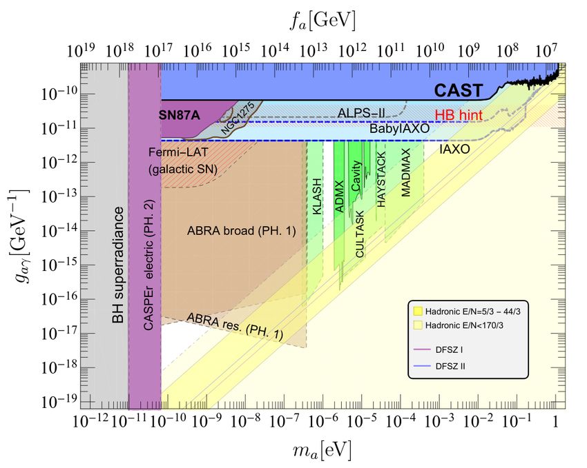
ically as long as Loff is small, we plot the axion-photon coupling as a function of axion
mass and decay constant in Fig. 1 together with the hints and existing as well as projected
constraints from various experiments and astrophysical observations.4 For reference, we
show axion-photon couplings in KSVZ models with heavy fermions in one representation
of the SM gauge group [47] and in DFSZ model.
3
By this notation we mean all integers from 1 to 7 excluding 3.
4
Hints and most constraints are discussed in detail in Ref. [43]. We present updated astrophysical
constraints from Ref. [44] together with the constraints derived from Chandra data on NGC 1275 [45] and
projected constraints from advanced LIGO [46].
– 11 –19 18 17 16 15 14 13 12 11 10 9 8 7
10 10 10 10 10 10 10 10 10 10 10 10 10
10 CAST
10
ALPS II
BabyIAXO
11 SN 1987A
10 IAXO
RF Cavity
aLIGO
MADMAX
HAYSTACK
12
10 Fermi-LAT
ADMX
(galactic SN)
13
KLASH
10
D
14 C
10 /
Q
S
d
A
Astrophysical constraints:
15 ABRACADABRA
10 NGC 1275 (Chandra)
broad (ph.1)
SN 1987A (Fermi)
16
10 NGC 1275, B t (Fermi)
ABR
ACA
DAB
R A re PKS 2155-304 (HESS)
17 s. ( Axion models:
ph
10 .1)
Astrophysical hints:
This work
Horizontal branch
18 KSVZ
10 TeV transparency
DFSZ
19
10
12 11 10 9 8 7 6 5 4 3 2 1
10 10 10 10 10 10 10 10 10 10 10 10 1
Figure 1. Axion-photon coupling as a function of axion mass and decay constant for various axion
models together with the existing and projected (dashed lines) constraints on the corresponding
parameter space from experiments as well as from astrophysical data. Astrophysical hints are also
shown. The dash-dotted line corresponds to the model of this work with the non-Abelian monopole
where the IR strong coupling αs value calculated in the AdS/QCD framework is adopted. The line
in the center of the vertically hatched band corresponds to the model with the minimal Abelian
monopole. For further discussion, see main text.
In Fig. 1, possible values for the axion-photon coupling in the model with the non-
Abelian monopole are organized in a vertically hatched band, while the model with the
minimal Abelian monopole yields a single line inside this band. The band denotes the
uncertainty we estimate for the model with the non-Abelian monopole, which is associated
to the dependence of the first line of Eq. (5.2) on the strong coupling αs in the IR. The
state of the art in studies of the behavior of the latter was discussed in detail in a recent
review [48], where it was shown that there exists a definition of αs in the IR, which is
analytic, independent of the choice of renormalization scheme or gauge, universal, based
on first principles and IR-finite (see Table 5.4 in Ref. [48]). This choice of definition for
IR αs corresponds to the so-called effective charges αg1 , αF3 and ατ , which are directly
related to the observables of low energy QCD. The measurements show that the IR strong
– 12 –coupling αs defined in such a way freezes at low energies. The freezing behavior of IR αs
is also supported by the success of the AdS/QCD technique in the description of hadron
properties [49]. Moreover, the value of the IR strong coupling calculated in AdS/QCD,
αAdS (0) = π, is consistent with the values αg1 (0) and αF3 (0) 5 . All this convinces us to
assume that the AdS/QCD value of IR strong coupling is a relevant one, that is why we
highlight the corresponding values of gaγ in Fig. 1 with a dash-dotted line. However, bearing
in mind that low energy QCD is still largely terra incognita, we allow for uncertainty in αs
which results in a band in Fig 1 where the lower edge αs (0) = 0.7 is chosen. Such choice is
suggested by the observation in Ref. [48] that most of the values of αs (0) in the literature
are clustered around αs (0) ∼ 3 (close to the AdS/QCD value) and αs (0) ∼ 0.7, not taking
into account the decoupling solution αs (0) = 0 disfavored for a number of reasons [50, 51].
Let us note as well that too large values of αs are disfavored by calculations in Ref. [52],
where it was shown that the magnetic coupling (i.e. the coupling inverse to αs ) never gets
too small in pure SU (2) gluodynamics, these results being extended to the pure SU (3) case
in Ref. [53].
Finally, let us mention that there is yet another source of uncertainty in our predictions,
both for the models with Abelian and non-Abelian monopoles, which is associated with the
U (1) magnetic charges of the monopoles. Whereas we consider them to be minimal in each
of the model, they are in principle not constrained by the stability arguments. This means
that gaγ can be further increased in Fig. 1 for the models of this work.
Next, let us consider axion couplings with matter, gai ≡ Cai mi /fa , where mi is the
mass of fermion i, which correspond to the following terms in the effective Lagrangian:
∂µ a
Leff ⊃ Cai ψ̄i γ µ γ5 ψi . (5.9)
2fa
As electrons do not carry PQ charge in the model we consider, the axion-electron coupling
gae is generated radiatively [54, 55]:
0 3α fa
gae = gaγ · me ln , (5.10)
2π me
where we took into account that the term associated to the axion-pion mixing is negligibly
small compared to the leading contribution. We find that the experiments and astrophysical
observations probing axion-electron interactions do not yield new constraints on the model.
Indeed, the CAST bound [56] on the axion-photon coupling, gaγ < 0.66 · 10−10 GeV−1 ,
constrains the phenomenologically viable region for axion-electron coupling: gae < 1.2 ·
10−16 ln fa /me . This constraint is stronger than any existing or projected bound from
interaction with electrons. As to the interactions of the axion with nucleons, it turns out
that contributions from radiatively generated axion-quark couplings are non-negligible and
actually enhance axion-nucleon couplings with respect to the conventional DFSZ case in
much of the parameter space. One can find that the coefficients Cap and Can are
Cap = −0.47 − 0.39 δcd + 0.88 δcu , (5.11)
Can = −0.02 + 0.88 δcd − 0.39 δcu , (5.12)
5
Although the effective charge ατ (0) is different, it is known that it contains an unsubtracted pion pole.
– 13 –where the numerical coefficients were calculated in [57] and the radiatively generated quark
couplings read as follows:
0 8α fa
δcu = gaγ fa · ln , (5.13)
27π mN
0 α fa
δcd = gaγ fa · ln , (5.14)
54π mN
where mN is the nucleon mass. Constraints on axion-neutron interactions are more stringent
than constraints on interactions with protons. We plot gan as a function of axion mass and
decay constant in Fig. 2 together with the constraint from neutron star cooling [58] and the
projected reach of the CASPEr Wind experiment [59]. For reference, we show the neutron-
axion coupling in DFSZ models, the range of which is constrained by the requirement of
perturbative unitarity of the Yukawa couplings of SM fermions [60]. Note that the slope of
the DFSZ band in Fig. 2 is different from the slope of the band corresponding to the axion
model of this paper. The difference arises because, in the DFSZ case, one obtains a linear
dependence of the coupling on the axion mass, gan ∝ ma , characteristic of the tree-level
couplings to quarks, while in the case of our model the linear dependence is superseded
by a nonlinear one, gan ∝ ma ln (const/ma ), due to the radiative origin of the coupling.
In Fig. 2, we show also the CAST bound [56] which is translated to a constraint on the
axion-neutron coupling with the use of Eqs. (5.12-5.14). Uncertainty in the prediction of
the axion-neutron coupling in the axion models of this work comes from the uncertainty in
the prediction of the axion-photon coupling, the latter being discussed at length above.
Finally, let us discuss if the axions we propose can comprise dark matter. In or-
der to avoid the cosmological magnetic monopole problem [61, 62], i.e. overproduction of
monopoles during the hot Big Bang epoch, we will set their masses and therefore the axion
decay constant fa to be larger than the reheating temperature. This means that we have to
deal only with the pre-inflationary scenario of axion dark matter production, which hinges
upon the misalignment mechanism [6–8]. Note that while Abelian dominance suggests that
the low temperature axion mass ma (fa ) is given approximately by the familiar expression
for the standard QCD axion, at higher temperatures, T & 1 GeV, the axion mass can
differ significantly from the standard case. The cosmic axion abundance resulting from the
misalignment production mechanism ρmis a is inversely proportional to the square root of the
axion mass at the moment where oscillations of the axion field start:
fa
ρmis
a ∝ p · F (Troll ) , (5.15)
ma (Troll )
where Troll is the temperature at which ma (Troll ) = 3H(Troll ), H being the Hubble expansion
rate, and F a fixed function of temperature. Due to Abelian dominance, we expect that
ρmis
a does not change too much with respect to the conventional QCD axion models if
Troll < 1 GeV. The latter condition can be recast into the form ma (GeV) < 3H(GeV),
which yields fa > 1012 GeV assuming the axion mass at 1 GeV is not much off the values
given in [63]. Combining it with the CAST bound, we see that in much of the allowed
parameter space axions produced via the misalignment mechanism have approximately the
– 14 –1019 1018 1017 1016 1015 1014 1013 1012 1011 1010 10 9 10 8 10 7
10 10
10 11 CASPEr Wind
10 12
10 13
10 14 Axion models:
This work
10 15 QCD DFSZ
S/
Ad
10 16
Existing constraints:
10 17 Neutron star cooling
10 18 Translated CAST bound
10 19 12 11
10 10 10 10 10 9 10 8 10 7 10 6 10 5 10 4 10 3 10 2 10 1 1
Figure 2. Axion-neutron coupling as a function of axion mass and decay constant for various ax-
ion models together with the existing and projected (dashed lines) constraints on the corresponding
parameter space from experiments as well as from astrophysical data. The dash-dotted line corre-
sponds to the model of this work with the non-Abelian monopole where the IR strong coupling αs
value calculated in the AdS/QCD framework is adopted. The line in the center of the vertically
hatched band corresponds to the model with the minimal Abelian monopole. For further discussion,
see main text.
same abundance as axions with the same mass in KSVZ and DFSZ-like models. The case
fa . 1012 GeV is more difficult: in order to infer the abundance of cosmic axions in the
model discussed, one has to calculate the axion mass as a function of temperature in the
energy range where there is no Abelian dominance. We leave a more thorough investigation
of axion cosmology in our model for future work.
6 Discussion
In this work, we introduced a new hadronic axion model which involves a very heavy vector-
like fermion magnetically charged under either the full non-Abelian symmetry of the low
energy SM or only its electromagnetic subgroup. We showed that both cases can realize the
PQ mechanism and thus provide a solution to the strong CP problem. We found that both
– 15 –cases lead to a very interesting phenomenology. Although we assumed Abelian dominance
in our discussion of phenomenology of the model with the non-Abelian monopole, it is easy
to see that the functions gaγ (fa ), gae (fa ) and gan (fa ) are independent of this assumption:
the latter two couplings are generated at 1-loop through the coupling to photons gaγ while
the axion-photon coupling is completely dominated by the aF F̃ term, see Eq. (5.5). The
quantities which are sensitive to the axion interactions with off-diagonal gluons are the axion
mass ma (fa ), the coupling to the nuclear EDM gd (fa ) and, in some part of the parameter
space, the couplings with protons and pions. If there exist non-vanishing quantum correc-
tions to the term Loff (Eq. (5.3)), the model with the non-Abelian monopole constitutes a
counterexample to the assertion of universality of axion-gluon coupling and EDM coupling
in QCD axion models. If such corrections are not too small, difference in EDM coupling
with respect to the conventional QCD axion models can offer an exciting opportunity of
distinguishing our axion model from the other QCD axion models in experiments such as
CASPEr Electric [59].
It is especially intriguing that the model of the QCD axion we discuss is consis-
tent with the astrophysical hints suggested both by anomalous TeV-transparency of the
Universe [17, 18] and by excessive cooling of horizontal branch stars in globular clus-
ters [16], see Fig. 1. Moreover, Fig. 1 shows that the parameter space of our model is
to be probed in the future by many experiments and astrophysical observatories, namely
ALPS II [64], BabyIAXO [65], IAXO [66] and Fermi-LAT [67]. Meanwhile, advanced
LIGO [46], KLASH [68] and ABRACADABRA [69] experiments have all the chances to
discover the cosmic abundance of such axions. As to the experiments which probe the
interactions of axion with neutrons, one can see in Fig. 2 that although the projected reach
of the CASPEr Wind experiment is not enough to probe the QCD axion model we propose,
the gap between theory and experiment is way smaller than in the case of DFSZ axions.
The model we discussed is peculiar in yet another way. Suppose that the axion is
found through its coupling with photons and that investigation of its EDM coupling shows
preference for the model involving non-Abelian monopole. Then one can infer the IR
strong coupling αs (0) by Eq. (5.2). This would be an independent experimental hint for
the coupling constant αs (0) which could refine other determinations.
Needless to say, it would be valuable to construct a UV completion to the model
discussed. Presence of heavy magnetic monopoles in the spectrum of the UV theory can
influence Z-boson physics, possibly providing an additional opportunity for probing the
model of this work experimentally. An interesting question regarding the UV completion
is whether the magnetic charges we discuss can emerge from some Grand Unified theory
via the ’t Hooft-Polyakov construction [70, 71]. Note that the model of this work requires
magnetic charges to be carried by fermionic particles. The latter can arise as systems of
magnetically and electrically charged bosons [72], e.g. as pairs of identical dyons. Fermionic
monopoles naturally arise in supersymmetric theories.
– 16 –A Axion-gluon coupling in the classical approximation
In this Appendix, we show that the axion-gluon coupling in the model with a heavy non-
Abelian monopole preserves its universality in the classical approximation, i.e. it is given
by the expression:
ags2
− Ga G̃a µν , (A.1)
32π 2 fa µν
so that Loff = 0 in Eq. (5.1), at least classicaly. We use the formalism of loop space
variables pioneered by Polyakov [73] and developed with the focus on the electric-magnetic
dual symmetry of the YM theory by Hong-Mo, Faridani and Tsun [29]. Central object of
the formalism is the parallel phase transport along the loop ξ(s), s ∈ [0, 2π] from one point
s1 to another s2 :
Z s2
Φξ (s2 , s1 ) = Ps exp igs ˙µ
ds Aµ (ξ(s)) ξ (s) , (A.2)
s1
where Ps is the Dyson ordering. Loop derivative of the holonomy defines the Polyakov
variables:
i δΦξ (2π, 0)
Fµ [ξ|s] = Φ−1
ξ (2π, 0) · , (A.3)
gs δξ µ (s)
which are known to constitute a valid set for a full description of the YM field [74, 75]. It
was shown in Ref. [29] that another complete set of variables is better suited for dealing
with the electric-magnetic dual symmetry of the classical YM theory, namely:
Eµ [ξ|s] = Φξ (s, 0) Fµ [ξ|s] Φ−1
ξ (s, 0) , (A.4)
which can be connected to the local quantities by the expression:
Z
−1 2
ω (x) G̃µν (x) ω (x) = µνρσ δξds E ρ [ξ|s] ξ˙σ (s) ξ˙−2 (s) δ(x − ξ(s)) , (A.5)
N
where ω (x) is an arbitrary local SU (3) matrix and N is a normalization factor. The dual
(d)
(magnetic) variables Eµ were shown to be related to the electric ones Eµ in the pure YM
theory in the following way:
Z
−1 2
(d)
ω (η(t)) Eµ [η|t] ω (η(t)) = µνρσ η̇ (t) δξds E ρ [ξ|s] ξ˙σ (s) ξ˙−2 (s) δ(ξ(s) − η(t)) ,
ν
N
(A.6)
while the inverse transformation is:
Z
2
ω(η(t)) Eµ [η|t] ω (η(t)) = − µνρσ η̇ (t) δξds E (d) ρ [ξ|s] ξ˙σ (s) ξ˙−2 (s) δ(ξ(s) − η(t)) .
−1 ν
N
(A.7)
Since in the derivation of the axion effective Lagrangian external fields can be considered
constant and homogeneous, as discussed in Sec. 4, we can apply Eqs. (A.6) and (A.7) in
order to find the relation between the expression A.1 and its dual analogue, constructed
– 17 –from the GNO group connection, in the classical theory. The calculation proceeds as follows:
Z Z n o
d x a(x) Gµν (x) G̃ (x) = 2 d4 x a(x) tr ω −1 (x) Gµν (x) ω (x) ω −1 (x) G̃µν (x) ω (x) =
4 a a µν
Z
8 n o
d4 x δξds a(x) tr ω −1 (x) G̃µν (x) ω (x) E µ [ξ|s] ξ˙ν (s) ξ˙−2 (s) δ(x − ξ(s)) =
N
Z
16
µνρσ δηdt δξds a(η(t)) tr {E ρ [η|t] E µ [ξ|s]} η̇ σ (t) η̇ −2 (t) ξ˙ν (s) ξ˙−2 (s) δ(η(t) − ξ(s)) =
N2
Z
8 n o
δηdt a(η(t)) tr E µ [η|t] ω −1 (η(t)) Eµ(d) [η|t] ω (η(t)) η̇ −2 (t) =
N
Z
8 n o
δηdt a(η(t)) tr ω (η(t)) E µ [η|t] ω −1 (η(t)) Eµ(d) [η|t] η̇ −2 (t) =
N
Z
16 n o
− 2 µνρσ δηdt δξds a(η(t)) tr Eρ(d) [η|t] Eµ(d) [ξ|s] η̇ σ (t) η̇ −2 (t) ξ˙ν (s) ξ˙−2 (s) δ(η(t) − ξ(s)) =
N
Z
− d4 x a(x) Ga(d) µν (x) G̃a(d)µν (x) (A.8)
where we took advantage of Eqs. (A.5), (A.6) and A.7, as well as of the cyclic property of
the trace. The last identity follows automatically as far as one notices that the third and
the sixth lines of the Eq. (A.8) are identical but for the overall sign and electric-magnetic
variables interchange. Now, one can clearly see that classically we recover the universal
axion-gluon coupling even in the model with the non-Abelian magnetic monopole:
ags2 ags2
Z Z
a µν
Seff, classical ⊃ d4 x G a
G̃
(d) µν (d) = − d4 x Ga G̃a µν . (A.9)
2
32π fa 32π 2 fa µν
Acknowlegments
We thank Claudio Bonati and Thomas Biekötter for discussions. A.R. acknowledges support
and A.S. is funded by the Deutsche Forschungsgemeinschaft (DFG, German Research Foun-
dation) under Germany’s Excellence Strategy – EXC 2121 Quantum Universe – 390833306.
References
[1] C. Abel et al. Measurement of the permanent electric dipole moment of the neutron. Phys.
Rev. Lett., 124(8):081803, 2020, 2001.11966.
[2] R.D. Peccei and Helen R. Quinn. CP Conservation in the Presence of Instantons. Phys. Rev.
Lett., 38:1440–1443, 1977.
[3] R.D. Peccei and Helen R. Quinn. Constraints Imposed by CP Conservation in the Presence
of Instantons. Phys. Rev. D, 16:1791–1797, 1977.
[4] Steven Weinberg. A New Light Boson? Phys. Rev. Lett., 40:223–226, 1978.
[5] Frank Wilczek. Problem of Strong P and T Invariance in the Presence of Instantons. Phys.
Rev. Lett., 40:279–282, 1978.
[6] John Preskill, Mark B. Wise, and Frank Wilczek. Cosmology of the Invisible Axion. Phys.
Lett. B, 120:127–132, 1983.
– 18 –[7] L.F. Abbott and P. Sikivie. A Cosmological Bound on the Invisible Axion. Phys. Lett. B,
120:133–136, 1983.
[8] Michael Dine and Willy Fischler. The Not So Harmless Axion. Phys. Lett. B, 120:137–141,
1983.
[9] Jihn E. Kim. Weak Interaction Singlet and Strong CP Invariance. Phys. Rev. Lett., 43:103,
1979.
[10] Mikhail A. Shifman, A.I. Vainshtein, and Valentin I. Zakharov. Can Confinement Ensure
Natural CP Invariance of Strong Interactions? Nucl. Phys. B, 166:493–506, 1980.
[11] Michael Dine, Willy Fischler, and Mark Srednicki. A Simple Solution to the Strong CP
Problem with a Harmless Axion. Phys. Lett. B, 104:199–202, 1981.
[12] A.R. Zhitnitsky. On Possible Suppression of the Axion Hadron Interactions. (In Russian).
Sov. J. Nucl. Phys., 31:260, 1980.
[13] Marco Farina, Duccio Pappadopulo, Fabrizio Rompineve, and Andrea Tesi. The photo-philic
QCD axion. JHEP, 01:095, 2017, 1611.09855.
[14] Anson Hook. Solving the Hierarchy Problem Discretely. Phys. Rev. Lett., 120(26):261802,
2018, 1802.10093.
[15] Luca Di Luzio, Belen Gavela, Pablo Quilez, and Andreas Ringwald. An even lighter QCD
axion. arXiv e-prints, Jan 2021, 2102.00012.
[16] Adrian Ayala, Inma Domínguez, Maurizio Giannotti, Alessandro Mirizzi, and Oscar
Straniero. Revisiting the bound on axion-photon coupling from Globular Clusters. Phys.
Rev. Lett., 113(19):191302, 2014, 1406.6053.
[17] A. De Angelis, O. Mansutti, M. Persic, and M. Roncadelli. Photon propagation and the
VHE gamma-ray spectra of blazars: how transparent is really the Universe? Mon. Not. Roy.
Astron. Soc., 394:L21–L25, 2009, 0807.4246.
[18] D. Horns and M. Meyer. Indications for a pair-production anomaly from the propagation of
VHE gamma-rays. JCAP, 02:033, 2012, 1201.4711.
[19] Paul Adrien Maurice Dirac. Quantised singularities in the electromagnetic field,. Proc. Roy.
Soc. Lond. A, 133(821):60–72, 1931.
[20] Daniel Zwanziger. Local-lagrangian quantum field theory of electric and magnetic charges.
Phys. Rev. D, 3:880–891, Feb 1971.
[21] Richard A. Brandt, Filippo Neri, and Daniel Zwanziger. Lorentz invariance of the quantum
field theory of electric and magnetic charge. Phys. Rev. Lett., 40:147–150, Jan 1978.
[22] Richard A. Brandt, Filippo Neri, and Daniel Zwanziger. Lorentz invariance from classical
particle paths in quantum field theory of electric and magnetic charge. Phys. Rev. D,
19:1153–1167, Feb 1979.
[23] V. A. Rubakov. Superheavy Magnetic Monopoles and Proton Decay. JETP Lett.,
33:644–646, 1981.
[24] Curtis G. Callan, Jr. Dyon-Fermion Dynamics. Phys. Rev. D, 26:2058–2068, 1982.
[25] F. Englert and Paul Windey. Quantization Condition for ’t Hooft Monopoles in Compact
Simple Lie Groups. Phys. Rev. D, 14:2728, 1976.
– 19 –[26] P. Goddard, J. Nuyts, and David I. Olive. Gauge Theories and Magnetic Charge. Nucl.
Phys. B, 125:1–28, 1977.
[27] C. Montonen and David I. Olive. Magnetic Monopoles as Gauge Particles? Phys. Lett. B,
72:117–120, 1977.
[28] Anton Kapustin and Edward Witten. Electric-Magnetic Duality And The Geometric
Langlands Program. Commun. Num. Theor. Phys., 1:1–236, 2007, hep-th/0604151.
[29] Hong-Mo Chan, J. Faridani, and Sheung-Tsun Tsou. A Generalized duality symmetry for
nonAbelian Yang-Mills fields. Phys. Rev. D, 53:7293–7305, 1996, hep-th/9512173.
[30] Tai Tsun Wu and Chen Ning Yang. Concept of Nonintegrable Phase Factors and Global
Formulation of Gauge Fields. Phys. Rev. D, 12:3845–3857, 1975.
[31] Richard A. Brandt and Filippo Neri. Stability Analysis for Singular Nonabelian Magnetic
Monopoles. Nucl. Phys. B, 161:253–282, 1979.
[32] Sidney R. Coleman. THE MAGNETIC MONOPOLE FIFTY YEARS LATER. In Les
Houches Summer School of Theoretical Physics: Laser-Plasma Interactions, 6 1982.
[33] Gerard ’t Hooft. Topology of the Gauge Condition and New Confinement Phases in
Nonabelian Gauge Theories. Nucl. Phys. B, 190:455–478, 1981.
[34] Claudio Bonati, Adriano Di Giacomo, Luca Lepori, and Fabrizio Pucci. Monopoles, abelian
projection and gauge invariance. Phys. Rev. D, 81:085022, 2010, 1002.3874.
[35] Kei-Ichi Kondo, Seikou Kato, Akihiro Shibata, and Toru Shinohara. Quark confinement:
Dual superconductor picture based on a non-Abelian Stokes theorem and reformulations of
Yang-Mills theory. Phys. Rept., 579:1–226, 2015, 1409.1599.
[36] Kazuhisa Amemiya and Hideo Suganuma. Off diagonal gluon mass generation and infrared
Abelian dominance in the maximally Abelian gauge in lattice QCD. Phys. Rev. D,
60:114509, 1999, hep-lat/9811035.
[37] Tsuneo Suzuki, Katsuya Ishiguro, and Vitaly Bornyakov. New scheme for color confinement
and violation of the non-Abelian Bianchi identities. Phys. Rev. D, 97(3):034501, 2018,
1712.05941. [Erratum: Phys.Rev.D 97, 099905 (2018)].
[38] Edward Witten. Dyons of Charge e theta/2 pi. Phys. Lett. B, 86:283–287, 1979.
[39] Cumrun Vafa and Edward Witten. Parity Conservation in QCD. Phys. Rev. Lett., 53:535,
1984.
[40] Julian S. Schwinger. On gauge invariance and vacuum polarization. Phys. Rev., 82:664–679,
1951.
[41] Tsuneo Suzuki and Ichiro Yotsuyanagi. A possible evidence for Abelian dominance in quark
confinement. Phys. Rev. D, 42:4257–4260, 1990.
[42] John D. Stack, Steven D. Neiman, and Roy J. Wensley. String tension from monopoles in
SU(2) lattice gauge theory. Phys. Rev. D, 50:3399–3405, 1994, hep-lat/9404014.
[43] Luca Di Luzio, Maurizio Giannotti, Enrico Nardi, and Luca Visinelli. The landscape of QCD
axion models. Phys. Rept., 870:1–117, 2020, 2003.01100.
[44] Gautham Adamane Pallathadka, Francesca Calore, Pierluca Carenza, Maurizio Giannotti,
Dieter Horns, Jhilik Majumdar, Alessandro Mirizzi, Andreas Ringwald, Anton Sokolov, and
Franziska Stief. Reconciling hints on axion-like-particles from high-energy gamma rays with
stellar bounds. arXiv e-prints, Aug 2020, 2008.08100.
– 20 –You can also read