GENERATIVE MODEL-ENHANCED HUMAN MOTION PREDICTION
←
→
Page content transcription
If your browser does not render page correctly, please read the page content below
Under review as a conference paper at ICLR 2021

G ENERATIVE                 MODEL - ENHANCED                         HUMAN             MOTION
PREDICTION

 Anonymous authors
 Paper under double-blind review

                                            A BSTRACT
         The task of predicting human motion is complicated by the natural heterogeneity
         and compositionality of actions, necessitating robustness to distributional shifts
         as far as out-of-distribution (OoD). Here we formulate a new OoD benchmark
         based on the Human3.6M and CMU motion capture datasets, and introduce a
         hybrid framework for hardening discriminative architectures to OoD failure by
         augmenting them with a generative model. When applied to current state-of-the-
         art discriminative models, we show that the proposed approach improves OoD
         robustness without sacrificing in-distribution performance, and can theoretically
         facilitate model interpretability. We suggest human motion predictors ought to
         be constructed with OoD challenges in mind, and provide an extensible general
         framework for hardening diverse discriminative architectures to extreme distribu-
         tional shift.

1   I NTRODUCTION
Human motion is naturally intelligible as a time-varying graph of connected joints constrained by
locomotor anatomy and physiology. Its prediction allows the anticipation of actions with appli-
cations across healthcare (Geertsema et al., 2018; Kakar et al., 2005), physical rehabilitation and
training (Chang et al., 2012; Webster & Celik, 2014), robotics (Koppula & Saxena, 2013b;a; Gui
et al., 2018b), navigation (Paden et al., 2016; Alahi et al., 2016; Bhattacharyya et al., 2018; Wang
et al., 2019), manufacture (Švec et al., 2014), entertainment (Shirai et al., 2007; Rofougaran et al.,
2018; Lau & Chan, 2008), and security (Kim & Paik, 2010; Ma et al., 2018).
The favoured approach to predicting movements over time has been purely inductive, relying on the
history of a specific class of movement to predict its future. For example, state space models (Koller
& Friedman, 2009) enjoyed early success for simple, common or cyclic motions (Taylor et al.,
2007; Sutskever et al., 2009; Lehrmann et al., 2014). The range, diversity and complexity of human
motion has encouraged a shift to more expressive, deep neural network architectures (Fragkiadaki
et al., 2015; Butepage et al., 2017; Martinez et al., 2017; Li et al., 2018; Aksan et al., 2019; Mao
et al., 2019; Li et al., 2020b; Cai et al., 2020), but still within a simple inductive framework.
This approach would be adequate were actions both sharply distinct and highly stereotyped. But
their complex, compositional nature means that within one category of action the kinematics may
vary substantially, while between two categories they may barely differ. Moreover, few real-world
tasks restrict the plausible repertoire to a small number of classes–distinct or otherwise–that could
be explicitly learnt. Rather, any action may be drawn from a great diversity of possibilities–both
kinematic and teleological–that shape the characteristics of the underlying movements. This has
two crucial implications. First, any modelling approach that lacks awareness of the full space of
motion possibilities will be vulnerable to poor generalisation and brittle performance in the face of
kinematic anomalies. Second, the very notion of In-Distribution (ID) testing becomes moot, for the
relations between different actions and their kinematic signatures are plausibly determinable only
across the entire domain of action. A test here arguably needs to be Out-of-Distribution (OoD) if it
is to be considered a robust test at all.
These considerations are amplified by the nature of real-world applications of kinematic modelling,
such as anticipating arbitrary deviations from expected motor behaviour early enough for an au-
tomatic intervention to mitigate them. Most urgent in the domain of autonomous driving (Bhat-
tacharyya et al., 2018; Wang et al., 2019), such safety concerns are of the highest importance, and

                                                  1
Under review as a conference paper at ICLR 2021

are best addressed within the fundamental modelling framework. Indeed, Amodei et al. (2016)
cites the ability to recognize our own ignorance as a safety mechanism that must be a core com-
ponent in safe AI. Nonetheless, to our knowledge, current predictive models of human kinematics
neither quantify OoD performance nor are designed with it in mind. There is therefore a need for
two frameworks, applicable across the domain of action modelling: one for hardening a predictive
model to anomalous cases, and another for quantifying OoD performance with established bench-
mark datasets. General frameworks are here desirable in preference to new models, for the field
is evolving so rapidly greater impact can be achieved by introducing mechanisms that can be ap-
plied to a breadth of candidate architectures, even if they are demonstrated in only a subset. Our
approach here is founded on combining a latent variable generative model with a standard predictive
model, illustrated with the current state-of-the-art discriminative architecture (Mao et al., 2019; Wei
et al., 2020), a strategy that has produced state-of-the-art in the medical imaging domain Myronenko
(2018). Our aim is to achieve robust performance within a realistic, low-volume, high-heterogeneity
data regime by providing a general mechanism for enhancing a discriminative architecture with a
generative model.
In short, our contributions to the problem of achieving robustness to distributional shift in human
motion prediction are as follows:

         1. We provide a framework to benchmark OoD performance on the most widely used open-
            source motion capture datasets: Human3.6M (Ionescu et al., 2013), and CMU-Mocap1 ,
            and evaluate state-of-the-art models on it.
         2. We present a framework for hardening deep feed-forward models to OoD samples. We
            show that the hardened models are fast to train, and exhibit substantially improved OoD
            performance with minimal impact on ID performance.

   We begin section 2 with a brief review of human motion prediction with deep neural networks,
and of OoD generalisation using generative models. In section 3, we define a framework for bench-
marking OoD performance using open-source multi-action datasets. We introduce in section 4 the
discriminative models that we harden using a generative branch to achieve a state-of-the-art (SOTA)
OoD benchmark. We then turn in section 5 to the architecture of the generative model and the overall
objective function. Section 6 presents our experiments and results. We conclude in section 7 with a
summary of our results, current limitations, and caveats, and future directions for developing robust
and reliable OoD performance and a quantifiable awareness of unfamiliar behaviour.

2       R ELATED W ORK

Deep-network based human motion prediction. Historically, sequence-to-sequence prediction
using Recurrent Neural Networks (RNNs) have been the de facto standard for human motion pre-
diction (Fragkiadaki et al., 2015; Jain et al., 2016; Martinez et al., 2017; Pavllo et al., 2018; Gui
et al., 2018a; Guo & Choi, 2019; Gopalakrishnan et al., 2019; Li et al., 2020b). Currently, the SOTA
is dominated by feed forward models (Butepage et al., 2017; Li et al., 2018; Mao et al., 2019; Wei
et al., 2020). These are inherently faster and easier to train than RNNs. The jury is still out, how-
ever, on the optimal way to handle temporality for human motion prediction. Meanwhile, recent
trends have overwhelmingly shown that graph-based approaches are an effective means to encode
the spatial dependencies between joints (Mao et al., 2019; Wei et al., 2020), or sets of joints (Li
et al., 2020b). In this study, we consider the SOTA models that have graph-based approaches with
a feed forward mechanism as presented by (Mao et al., 2019), and the subsequent extension which
leverages motion attention, Wei et al. (2020). We show that these may be augmented to improve
robustness to OoD samples.

Generative models for Out-of-Distribution prediction and detection. Despite the power of
deep neural networks for prediction in complex domains (LeCun et al., 2015), they face several
challenges that limits their suitability for safety-critical applications. Amodei et al. (2016) list ro-
bustness to distributional shift as one of the five major challenges to AI safety. Deep generative
models, have been used extensively for detection of OoD inputs and have been shown to generalise
    1
        t http://mocap.cs.cmu.edu/

                                                   2
Under review as a conference paper at ICLR 2021

well in such scenarios (Hendrycks & Gimpel, 2016; Liang et al., 2017; Hendrycks et al., 2018).
While recent work has showed some failures in simple OoD detection using density estimates from
deep generative models (Nalisnick et al., 2018; Daxberger & Hernández-Lobato, 2019), they remain
a prime candidate for anomaly detection (Kendall & Gal, 2017; Grathwohl et al., 2019; Daxberger
& Hernández-Lobato, 2019).
Myronenko (2018) use a Variational Autoencoder (VAE) (Kingma & Welling, 2013) to regularise an
encoder-decoder architecture with the specific aim of better generalisation. By simultaneously using
the encoder as the recognition model of the VAE, the model is encouraged to base its segmentations
on a complete picture of the data, rather than on a reductive representation that is more likely to
be fitted to the training data. Furthermore, the original loss and the VAE’s loss are combined as a
weighted sum such that the discriminator’s objective still dominates. Further work may also reveal
useful interpretability of behaviour (via visualisation of the latent space as in Bourached & Nachev
(2019)), generation of novel motion (Motegi et al., 2018), or reconstruction of missing joints as in
Chen et al. (2015).

3     Q UANTIFYING OUT- OF - DISTRIBUTION PERFORMANCE OF HUMAN MOTION
      PREDICTORS

Even a very compact representation of the human body such as OpenPose’s 17 joint parameterisation
Cao et al. (2018) explodes to unmanageable complexity when a temporal dimension is introduced of
the scale and granularity necessary to distinguish between different kinds of action: typically many
seconds, sampled at hundredths of a second. Moreover, though there are anatomical and physio-
logical constraints on the space of licit joint configurations, and their trajectories, the repertoire of
possibility remains vast, and the kinematic demarcations of teleologically different actions remain
indistinct. Thus, no practically obtainable dataset may realistically represent the possible distance
between instances. To simulate OoD data we first need ID data that can be varied in its quantity and
heterogeneity, closely replicating cases where a particular kinematic morphology may be rare, and
therefore undersampled, and cases where kinematic morphologies are both highly variable within a
defined class and similar across classes. Such replication needs to accentuate the challenging aspects
of each scenario.
We therefore propose to evaluate OoD performance where only a single action, drawn from a single
action distribution, is available for training and hyperparameter search, and testing is carried out on
the remaining classes. In appendix A, to show that the action categories we have chosen can be
distinguished at the time scales on which our trajectories are encoded, we train a simple classifier
and show it separates the selected ID action from the others with high accuracy (100% precision and
recall for the CMU dataset). Performance over the remaining set of actions may thus be considered
OoD.

4     BACKGROUND
Here we describe the current SOTA model proposed by Mao et al. (2019) (GCN). We then describe
the extension by Wei et al. (2020) (attention-GCN) which antecedes the GCN prediction model with
motion attention.

4.1   P ROBLEM F ORMULATION

We are given a motion sequence X1:N = (x1 , x2 , x3 , · · · , xN ) consisting of N consecutive human
poses, where xi ∈ RK , with K the number of parameters describing each pose. The goal is to
predict the poses XN +1:N +T for the subsequent T time steps.

4.2   DCT- BASED T EMPORAL E NCODING

The input is transformed using Discrete Cosine Transformations (DCT). In this way each resulting
coefficient encodes information of the entire sequence at a particular temporal frequency. Further-
more, the option to remove high or low frequencies is provided. Given a joint, k, the position of k
over N time steps is given by the trajectory vector: xk = [xk,1 , . . . , xk,N ] where we convert to a

                                                   3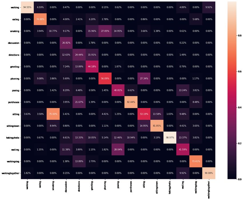
Under review as a conference paper at ICLR 2021

DCT vector of the form: Ck = [Ck,1 , . . . , Ck,N ] where Ck,l represents the lth DCT coefficient. For
δl1 ∈ RN = [1, 0, · · · , 0], these coefficients may be computed as

                                r      N
                                    2 X            1          π
                      Ck,l =              xk,n √         cos     (2n − 1)(l − 1) .                              (1)
                                    N n=1        1 + δl1      2N

If no frequencies are cropped, the DCT is invertible via the Inverse Discrete Cosine Transform
(IDCT):

                                r     N
                                    2 X          1          π
                       xk,l =           Ck,l √         cos     (2n − 1)(l − 1) .                                (2)
                                    N          1 + δl1      2N
                                      l=1

Mao et al. use the DCT transform with a graph convolutional network architecture to predict the
output sequence. This is achieved by having an equal length input-output sequence, where the input
is the DCT transformation of xk = [xk,1 , . . . , xk,N , xk,N +1 , . . . , xk,N +T ], here [xk,1 , . . . , xk,N ] is
the observed sequence and [xk,N +1 , . . . , xk,N +T ] are replicas of xk,N (ie xk,n = xk,N for n ≥ N ).
The target is now simply the ground truth xk .

4.3    G RAPH C ONVOLUTIONAL N ETWORK

Suppose C ∈ RK×(N +T ) is defined on a graph with k nodes and N + T dimensions, then we define
a graph convolutional network to respect this structure. First we define a Graph Convolutional Layer
(GCL) that, as input, takes the activation of the previous layer (A[l−1] ), where l is the current layer.

                                      GCL(A[l−1] ) = SA[l−1] W + b                                              (3)

where A[0] = C ∈ RK×(N +T ) , and S ∈ RK×K is a layer-specific learnable normalised graph
                                                            [l−1]
                                                                  ×n[l]
laplacian that represents connections between joints, W ∈ Rn            are the learnable inter-layer
                        [l]
weightings and b ∈ Rn are the learnable biases where n[l] are the number of hidden units in layer
l.

4.4    N ETWORK S TRUCTURE AND L OSS

The network consists of 12 Graph Convolutional Blocks (GCBs), each containing 2 GCLs with
skip (or residual) connections, see figure 7. Additionally, there is one GCL at the beginning of the
network, and one at the end. n[l] = 256, for each layer, l. There is one final skip connection from
the DCT inputs to the DCT outputs, which greatly reduces train time. The model has around 2.6M
parameters. Hyperbolic tangent functions are used as the activation function. Batch normalisation
is applied before each activation.
The outputs are converted back to their original coordinate system using the IDCT (equation 2) to
be compared to the ground truth. The loss used for joint angles is the average l1 distance between
the ground-truth joint angles, and the predicted ones. Thus, the joint angle loss is:

                                                   N    K
                                                     +T X
                                            1      X
                                  `a =                    |x̂k,n − xk,n |                                       (4)
                                         K(N + T ) n=1
                                                             k=1

where x̂k,n is the predicted k th joint at timestep n and xk,n is the corresponding ground truth.
This is separately trained on 3D joint coordinate prediction making use of the Mean Per Joint Posi-
tion Error (MPJPE), as proposed in Ionescu et al. (2013) and used in Mao et al. (2019); Wei et al.
(2020). This is defined, for each training example, as

                                                         4
Under review as a conference paper at ICLR 2021
GCL 6 × GCB 6 × GCB GCL
K K K K K + K
20 256 256 256 20 20
GCL
GCL
K + K ·
GCL( K ) = K × K × 20
L 16 16 16
20 K 20 µ σ
K
GCL
20
GCL 6 × GCB
GCB( K ) = K + K × K × K × 20
256
× 256 K K K
µrecon
20 20 K K 20 16 256 256
z
K
GCL
20
256 σrecon
Figure 1: GCN network architecture with VAE branch. Here nz = 16 is the number of latent
variables per joint.
N J
+T X
1 X 2
`m = kp̂j,n − pj,n k (5)
J(N + T ) n=1 j=1
where p̂j,n ∈ R3 denotes the predicted jth joint position in frame n. And pj,n is the corresponding
ground truth, while J is the number of joints in the skeleton.
4.5 M OTION ATTENTION EXTENSION
Wei et al. (2020) extend this model by summing multiple DCT transformations from different sec-
tions of the motion history with weightings learned via an attention mechanism. For this extension,
the above model (the GCN) along with the anteceding motion attention is trained end-to-end. We
refer to this as the attention-GCN.
5 O UR A PPROACH
Myronenko (2018) augment an encoder-decoder discriminative model by using the encoder as a
recognition model for a Variational Autoencoder (VAE), (Kingma & Welling, 2013; Rezende et al.,
2014). Myronenko (2018) show this to be a very effective regulariser. Here, we also use a VAE,
but for conjugacy with the discriminator, we use graph convolutional layers in the decoder. This can
be compared to the Variational Graph Autoencoder (VGAE), proposed by Kipf & Welling (2016).
However, Kipf & Welling’s application is a link prediction task in citation networks and thus it is
desired to model only connectivity in the latent space. Here we model connectivity, position, and
temporal frequency. To reflect this distinction, the layers immediately before, and after, the latent
space are fully connected creating a homogenous latent space.
The generative model sets a precedence for information that can be modelled causally, while leaving
elements of the discriminative machinery, such as skip connections, to capture correlations that
remain useful for prediction but are not necessarily persuant to the objective of the generative model.
In addition to performing the role of regularisation in general, we show that we gain robustness to
distributional shift across similar, but different, actions that are likely to share generative properties.
The architecture may be considered with the visual aid in figure 1.
5.1 VARIATIONAL AUTOENCODER (VAE) B RANCH AND L OSS
Here we define the first 6 GCB blocks as our VAE recognition model, with a latent variable z ∈
RK×nz = N (µz , σz ), where µz ∈ RK×nz , σz ∈ RK×nz . nz = 8, or 32 depending on training
stability.
The KL divergence between the latent space distribution and a spherical Gaussian N (0, I) is given
by:
5Under review as a conference paper at ICLR 2021
nz
1X
µz 2 + σz 2 − 1 − log((σz )2 ) .
`l = KL(q(Z|C)||q(Z)) = (6)
2 1
The decoder part of the VAE has the same structure as the discriminative branch; 6 GCBs. We
parametrise the output neurons as µ ∈ RK×(N +T ) , and log(σ 2 ) ∈ RK×(N +T ) . We can now model
the reconstruction of inputs as samples of a maximum likelihood of a Gaussian distribution which
constitutes the second term of the negative Variational Lower Bound (VLB) of the VAE:
N +T K
!
2
1 XX 2 |Ck,l − µk,l |
`G = log(p(C|Z)) = − log(σk,l ) + log(2π) + 2 , (7)
2 n=1
l=1 elog(σk,l )
where Ck,l are the DCT coefficients of the ground truth.
5.2 T RAINING
We train the entire network together with the additional of the negative VLB:
N +T XK
1 X
`= |x̂k,n − xk,n | −λ (`G − `l ) . (8)
(N + T )K n=1 | {z }
k=1
| {z } VLB
Discriminitive loss
Here λ is a hyperparameter of the model. The overall network is ≈ 3.4M parameters. The number
of parameters varies slightly as per the number of joints, K, since this is reflected in the size of the
graph in each layer (k = 48 for H3.6M, K = 64 for CMU joint angles, and K = J = 75 for
CMU Cartesian coordinates). Furthermore, once trained, the generative model is not required for
prediction and hence for this purpose is as compact as the original models.
6 E XPERIMENTS
6.1 DATASETS AND E XPERIMENTAL S ETUP
Human3.6M (H3.6M) The H3.6M dataset (Ionescu et al., 2011; 2013), so called as it contains a
selection of 3.6 million 3D human poses and corresponding images, consists of seven actors each
performing 15 actions, such as walking, eating, discussion, sitting, and talking on the phone. Mar-
tinez et al. (2017); Mao et al. (2019); Li et al. (2020b) all follow the same training and evaluation
procedure: training their motion prediction model on 6 (5 for train and 1 for cross-validation) of the
actors, for each action, and evaluate metrics on the final actor, subject 5. For easy comparison to
these ID baselines, we maintain the same train; cross-validation; and test splits. However, we use
the single, most well-defined action (see appendix A), walking, for train and cross-validation, and
we report test error on all the remaining actions from subject 5. In this way we conduct all parameter
selection based on ID performance.
CMU motion capture (CMU-mocap) The CMU dataset consists of 5 general classes of actions.
Similarly to (Li et al., 2018; 2020a; Mao et al., 2019) we use 8 detailed actions from these classes:
’basketball’, ’basketball signal’, ’directing traffic’ ’jumping, ’running’, ’soccer’, ’walking’, and
’window washing’. We use two representations, a 64-dimensional vector that gives an exponen-
tial map representation (Grassia, 1998) of the joint angle, and a 75-dimensional vector that gives the
3D Cartesian coordinates of 25 joints. We do not tune any hyperparameters on this dataset and use
only a train and test set with the same split as is common in the literature (Martinez et al., 2017;
Mao et al., 2019).
6Under review as a conference paper at ICLR 2021
Model configuration We implemented the model in PyTorch (Paszke et al., 2017) using the
ADAM optimiser (Kingma & Ba, 2014). The learning rate was set to 0.0005 for all experiments
where, unlike Mao et al. (2019); Wei et al. (2020), we did not decay the learning rate as it was hy-
pothesised that the dynamic relationship between the discriminative and generative loss would make
this redundant. The batch size was 16. For numerical stability, gradients were clipped to a maximum
`2-norm of 1 and log(σ̂ 2 ) and values were clamped between -20 and 3. Code for all experiments
is available at the following anonymized link: https://anonymous.4open.science/r/11a7a2b5-da13-
43f8-80de-51e526913dd2/
Walking (ID) Eating (OoD) Smoking (OoD) Average (of 14 for OoD)
milliseconds 80 160 320 400 80 160 320 400 80 160 320 400 80 160 320 400
GCN (OoD) 0.22 0.37 0.60 0.65 0.22 0.38 0.65 0.79 0.28 0.55 1.08 1.10 0.38 0.69 1.09 1.27
Std Dev 0.001 0.008 . 0.008 0.01 0.003 0.01 0.03 0.04 0.01 0.01 0.02 0.02 0.007 0.02 0.04 0.04
ours (OoD) 0.23 0.37 0.59 0.64 0.21 0.37 0.59 0.72 0.28 0.54 1.01 0.99 0.38 0.68 1.07 1.21
Std Dev 0.003 0.004 0.03 0.03 0.008 0.01 0.03 0.04 0.005 0.01 0.01 0.02 0.006 0.01 0.01 0.02
Table 1: Short-term prediction of Eucildean distance between predicted and ground truth joint angles
on H3.6M. Each experiment conducted 3 times. We report the mean and standard deviation. Note
that we have lower variance in results for ours. Full table in appendix, table 6.
Walking Eating Smoking Discussion Average
milliseconds 560 1000 560 1000 560 1000 560 1000 560 1000
GCN (OoD) 0.80 0.80 0.89 1.20 1.26 1.85 1.45 1.88 1.10 1.43
ours (OoD) 0.66 0.72 0.90 1.19 1.17 1.78 1.44 1.90 1.04 1.40
Table 2: Long-term prediction of Eucildean distance between predicted and ground truth joint angles
on H3.6M.
Baseline comparison Both Mao et al. (2019) (GCN), and Wei et al. (2020) (attention-GCN) use
this same Graph Convolutional Network (GCN) architecture with DCT inputs. In particular, Wei
et al. (2020) increase the amount of history accounted for by the GCN by adding a motion attention
mechanism to weight the DCT coefficients from different sections of the history prior to being
inputted to the GCN. We compare against both of these baselines on OoD actions. For attention-
GCN we leave the attention mechanism preceding the GCN unchanged such that the generative
branch of the model is reconstructing the weighted DCT inputs to the GCN, and the whole network
is end-to-end differentiable.
Hyperparameter search Since a new term has been introduced to the loss function, it was neces-
sary to determine a sensible weighting between the discriminative and generative models. In Myro-
nenko (2018), this weighting was arbitrarily set to 0.1. It is natural that the optimum value here will
relate to the other regularisation parameters in the model. Thus, we conducted random hyperparam-
eter search for pdrop and λ in the ranges pdrop = [0, 0.5] on a linear scale, and λ = [10, 0.00001]
on a logarithmic scale. For fair comparison we also conducted hyperparameter search on GCN, for
values of the dropout probability (pdrop ) between 0.1 and 0.9. For each model, 25 experiments were
run and the optimum values were selected on the lowest ID validation error. The hyperparameter
search was conducted only for the GCN model on short-term predictions for the H3.6M dataset and
used for all future experiments hence demonstrating generalisability of the architecture.
6.2 R ESULTS
Basketball (ID) Basketball Signal (OoD) Average (of 7 for OoD)
milliseconds 80 160 320 400 1000 80 160 320 400 1000 80 160 320 400 1000
GCN 0.40 0.67 1.11 1.25 1.63 0.27 0.55 1.14 1.42 2.18 0.36 0.65 1.41 1.49 2.17
ours 0.40 0.66 1.12 1.29 1.76 0.28 0.57 1.15 1.43 2.07 0.34 0.62 1.35 1.41 2.10
Table 3: Eucildean distance between predicted and ground truth joint angles on CMU. Full table in
appendix, table 7.
Consistent with the literature we report short-term (< 500ms) and long-term (> 500ms) predic-
tions. In comparison to GCN, we take short term history into account (10 frames, 400ms) for both
7Under review as a conference paper at ICLR 2021
Basketball Basketball Signal Average (of 7 for OoD)
milliseconds 80 160 320 400 1000 80 160 320 400 1000 80 160 320 400 1000
GCN (OoD) 15.7 28.9 54.1 65.4 108.4 14.4 30.4 63.5 78.7 114.8 20.0 43.8 86.3 105.8 169.2
ours (OoD) 16.0 30.0 54.5 65.5 98.1 12.8 26.0 53.7 67.6 103.2 21.6 42.3 84.2 103.8 164.3
Table 4: Mean Joint Per Position Error (MPJPE) between predicted and ground truth 3D Cartesian
coordinates of joints on CMU. Full table in appendix, table 8.
datasets to predict both short- and long-term motion. In comparison to attention-GCN, we take long
term history (50 frames, 2 seconds) to predict the next 10 frames, and predict futher into the future
by recursively applying the predictions as input to the model as in Wei et al. (2020). In this way a
single short term prediction model may produce long term predictions.
We use Euclidean distance between the predicted and ground-truth joint angles for the Euler angle
representation. For 3D joint coordinate representation we use the MPJPE as used for training (equa-
tion 5). Table 1 reports the joint angle error for the short term predictions on the H3.6M dataset.
Here we found the optimum hyperparameters to be pdrop = 0.5 for GCN, and λ = 0.003, with
pdrop = 0.3 for our augmentation of GCN. The latter of which was used for all future experi-
ments, where for our augmentation of attention-GCN we removed dropout altogether. On average,
our model performs convincingly better both ID and OoD. Here the generative branch works well
as both a regulariser for small datasets and by creating robustness to distributional shifts. We see
similar and consistent results for long-term predictions in table 2.
From tables 3 and 4, we can see that the superior OoD performance generalises to the CMU dataset
with the same hyperparameter settings with a similar trend of the difference being larger for longer
predictions for both joint angles and 3D joint coordinates. For each of these experiments nz = 8.
Table 5, shows that the effectiveness of the generative branch generalises to the very recent motion
attention architecture. For attention-GCN we used nz = 32. Here, interestingly short term pre-
dictions are poor but long term predictions are consistently better. This supports our assertion that
information relevant to generative mechanisms are more intrinsic to the causal model and thus, here,
when the predicted output is recursively used, more useful information is available for the future
predictions.
Walking (ID) Eating (OoD) Smoking (OoD) Average (of 14 for OoD)
milliseconds 560 720 880 1000 560 720 880 1000 560 720 880 1000 560 720 880 1000
att-GCN (OoD) 55.4 60.5 65.2 68.7 87.6 103.6 113.2 120.3 81.7 93.7 102.9 108.7 112.1 129.6 140.3 147.8
ours (OoD) 58.7 60.6 65.5 69.1 81.7 94.4 102.7 109.3 80.6 89.9 99.2 104.1 113.1 127.7 137.9 145.3
Table 5: Long-term prediction of 3D joint positions on H3.6M. Here, ours is also trained with the
attention-GCN model. Full table in appendix, table 9.
7 C ONCLUSION
We draw attention to the need for robustness to distributional shifts in predicting human motion,
and propose a framework for its evaluation based on major open source datasets. We demonstrate
that state-of-the-art discriminative architectures can be hardened to extreme distributional shifts by
augmentation with a generative model, combining low in-distribution predictive error with maximal
generalisability. The introduction of a surveyable latent space further provides a mechanism for
model perspicuity and interpretability, and explicit estimates of uncertainty facilitate the detection
of anomalies: both characteristics are of substantial value in emerging applications of motion pre-
diction, such as autonomous driving, where safety is paramount. Our investigation argues for wider
use of generative models in behavioural modelling, and shows it can be done with minimal or no
performance penalty, within hybrid architectures of potentially diverse constitution.
8Under review as a conference paper at ICLR 2021
R EFERENCES
Emre Aksan, Manuel Kaufmann, and Otmar Hilliges. Structured prediction helps 3d human motion
modelling. In Proceedings of the IEEE International Conference on Computer Vision, pp. 7144–
7153, 2019.
Alexandre Alahi, Kratarth Goel, Vignesh Ramanathan, Alexandre Robicquet, Li Fei-Fei, and Silvio
Savarese. Social lstm: Human trajectory prediction in crowded spaces. In Proceedings of the
IEEE conference on computer vision and pattern recognition, pp. 961–971, 2016.
Dario Amodei, Chris Olah, Jacob Steinhardt, Paul Christiano, John Schulman, and Dan Mané. Con-
crete problems in ai safety. arXiv preprint arXiv:1606.06565, 2016.
Apratim Bhattacharyya, Mario Fritz, and Bernt Schiele. Long-term on-board prediction of people
in traffic scenes under uncertainty. In Proceedings of the IEEE Conference on Computer Vision
and Pattern Recognition, pp. 4194–4202, 2018.
Anthony Bourached and Parashkev Nachev. Unsupervised videographic analysis of rodent be-
haviour. arXiv preprint arXiv:1910.11065, 2019.
Judith Butepage, Michael J Black, Danica Kragic, and Hedvig Kjellstrom. Deep representation
learning for human motion prediction and classification. In Proceedings of the IEEE conference
on computer vision and pattern recognition, pp. 6158–6166, 2017.
Yujun Cai, Lin Huang, Yiwei Wang, Tat-Jen Cham, Jianfei Cai, Junsong Yuan, Jun Liu, Xu Yang,
Yiheng Zhu, Xiaohui Shen, et al. Learning progressive joint propagation for human motion pre-
diction. In Proceedings of the European Conference on Computer Vision (ECCV), 2020.
Zhe Cao, Gines Hidalgo, Tomas Simon, Shih-En Wei, and Yaser Sheikh. Openpose: realtime multi-
person 2d pose estimation using part affinity fields. arXiv preprint arXiv:1812.08008, 2018.
Chien-Yen Chang, Belinda Lange, Mi Zhang, Sebastian Koenig, Phil Requejo, Noom Somboon,
Alexander A Sawchuk, and Albert A Rizzo. Towards pervasive physical rehabilitation using
microsoft kinect. In 2012 6th international conference on pervasive computing technologies for
healthcare (PervasiveHealth) and workshops, pp. 159–162. IEEE, 2012.
Nutan Chen, Justin Bayer, Sebastian Urban, and Patrick Van Der Smagt. Efficient movement repre-
sentation by embedding dynamic movement primitives in deep autoencoders. In 2015 IEEE-RAS
15th International Conference on Humanoid Robots (Humanoids), pp. 434–440. IEEE, 2015.
Erik Daxberger and José Miguel Hernández-Lobato. Bayesian variational autoencoders for unsu-
pervised out-of-distribution detection. arXiv preprint arXiv:1912.05651, 2019.
Katerina Fragkiadaki, Sergey Levine, Panna Felsen, and Jitendra Malik. Recurrent network models
for human dynamics. In Proceedings of the IEEE International Conference on Computer Vision,
pp. 4346–4354, 2015.
Evelien E Geertsema, Roland D Thijs, Therese Gutter, Ben Vledder, Johan B Arends, Frans S
Leijten, Gerhard H Visser, and Stiliyan N Kalitzin. Automated video-based detection of nocturnal
convulsive seizures in a residential care setting. Epilepsia, 59:53–60, 2018.
Anand Gopalakrishnan, Ankur Mali, Dan Kifer, Lee Giles, and Alexander G Ororbia. A neural tem-
poral model for human motion prediction. In Proceedings of the IEEE Conference on Computer
Vision and Pattern Recognition, pp. 12116–12125, 2019.
F Sebastian Grassia. Practical parameterization of rotations using the exponential map. Journal of
graphics tools, 3(3):29–48, 1998.
Will Grathwohl, Kuan-Chieh Wang, Jörn-Henrik Jacobsen, David Duvenaud, Mohammad Norouzi,
and Kevin Swersky. Your classifier is secretly an energy based model and you should treat it like
one. arXiv preprint arXiv:1912.03263, 2019.
Liang-Yan Gui, Yu-Xiong Wang, Xiaodan Liang, and José MF Moura. Adversarial geometry-
aware human motion prediction. In Proceedings of the European Conference on Computer Vision
(ECCV), pp. 786–803, 2018a.
9Under review as a conference paper at ICLR 2021
Liang-Yan Gui, Kevin Zhang, Yu-Xiong Wang, Xiaodan Liang, José MF Moura, and Manuela
Veloso. Teaching robots to predict human motion. In 2018 IEEE/RSJ International Conference
on Intelligent Robots and Systems (IROS), pp. 562–567. IEEE, 2018b.
Xiao Guo and Jongmoo Choi. Human motion prediction via learning local structure representations
and temporal dependencies. In Proceedings of the AAAI Conference on Artificial Intelligence,
volume 33, pp. 2580–2587, 2019.
Dan Hendrycks and Kevin Gimpel. A baseline for detecting misclassified and out-of-distribution
examples in neural networks. arXiv preprint arXiv:1610.02136, 2016.
Dan Hendrycks, Mantas Mazeika, and Thomas Dietterich. Deep anomaly detection with outlier
exposure. arXiv preprint arXiv:1812.04606, 2018.
Catalin Ionescu, Fuxin Li, and Cristian Sminchisescu. Latent structured models for human pose
estimation. In 2011 International Conference on Computer Vision, pp. 2220–2227. IEEE, 2011.
Catalin Ionescu, Dragos Papava, Vlad Olaru, and Cristian Sminchisescu. Human3.6m: Large scale
datasets and predictive methods for 3d human sensing in natural environments. IEEE transactions
on pattern analysis and machine intelligence, 36(7):1325–1339, 2013.
Ashesh Jain, Amir R Zamir, Silvio Savarese, and Ashutosh Saxena. Structural-rnn: Deep learning
on spatio-temporal graphs. In Proceedings of the ieee conference on computer vision and pattern
recognition, pp. 5308–5317, 2016.
Manish Kakar, Håkan Nyström, Lasse Rye Aarup, Trine Jakobi Nøttrup, and Dag Rune Olsen.
Respiratory motion prediction by using the adaptive neuro fuzzy inference system (anfis). Physics
in Medicine & Biology, 50(19):4721, 2005.
Alex Kendall and Yarin Gal. What uncertainties do we need in bayesian deep learning for computer
vision? In Advances in neural information processing systems, pp. 5574–5584, 2017.
Daehee Kim and J Paik. Gait recognition using active shape model and motion prediction. IET
Computer Vision, 4(1):25–36, 2010.
Diederik P Kingma and Jimmy Ba. Adam: A method for stochastic optimization. arXiv preprint
arXiv:1412.6980, 2014.
Diederik P Kingma and Max Welling. Auto-encoding variational bayes. arXiv preprint
arXiv:1312.6114, 2013.
Thomas N Kipf and Max Welling. Variational graph auto-encoders. arXiv preprint
arXiv:1611.07308, 2016.
Daphne Koller and Nir Friedman. Probabilistic graphical models: principles and techniques. MIT
press, 2009.
Hema Koppula and Ashutosh Saxena. Learning spatio-temporal structure from rgb-d videos for
human activity detection and anticipation. In International conference on machine learning, pp.
792–800, 2013a.
Hema Swetha Koppula and Ashutosh Saxena. Anticipating human activities for reactive robotic
response. In IROS, pp. 2071. Tokyo, 2013b.
Rynson WH Lau and Addison Chan. Motion prediction for online gaming. In International Work-
shop on Motion in Games, pp. 104–114. Springer, 2008.
Yann LeCun, Yoshua Bengio, and Geoffrey Hinton. Deep learning. nature, 521(7553):436–444,
2015.
Andreas M Lehrmann, Peter V Gehler, and Sebastian Nowozin. Efficient nonlinear markov models
for human motion. In Proceedings of the IEEE Conference on Computer Vision and Pattern
Recognition, pp. 1314–1321, 2014.
10Under review as a conference paper at ICLR 2021
Chen Li, Zhen Zhang, Wee Sun Lee, and Gim Hee Lee. Convolutional sequence to sequence model
for human dynamics. In Proceedings of the IEEE Conference on Computer Vision and Pattern
Recognition, pp. 5226–5234, 2018.
Dongxu Li, Cristian Rodriguez, Xin Yu, and Hongdong Li. Word-level deep sign language recog-
nition from video: A new large-scale dataset and methods comparison. In Proceedings of the
IEEE/CVF Winter Conference on Applications of Computer Vision (WACV), March 2020a.
Maosen Li, Siheng Chen, Yangheng Zhao, Ya Zhang, Yanfeng Wang, and Qi Tian. Dynamic mul-
tiscale graph neural networks for 3d skeleton based human motion prediction. In Proceedings of
the IEEE/CVF Conference on Computer Vision and Pattern Recognition, pp. 214–223, 2020b.
Shiyu Liang, Yixuan Li, and Rayadurgam Srikant. Enhancing the reliability of out-of-distribution
image detection in neural networks. arXiv preprint arXiv:1706.02690, 2017.
Zhuo Ma, Xinglong Wang, Ruijie Ma, Zhuzhu Wang, and Jianfeng Ma. Integrating gaze tracking
and head-motion prediction for mobile device authentication: A proof of concept. Sensors, 18(9):
2894, 2018.
Wei Mao, Miaomiao Liu, Mathieu Salzmann, and Hongdong Li. Learning trajectory dependencies
for human motion prediction. In Proceedings of the IEEE International Conference on Computer
Vision, pp. 9489–9497, 2019.
Julieta Martinez, Michael J Black, and Javier Romero. On human motion prediction using recur-
rent neural networks. In Proceedings of the IEEE Conference on Computer Vision and Pattern
Recognition, pp. 2891–2900, 2017.
Leland McInnes, John Healy, and James Melville. Umap: Uniform manifold approximation and
projection for dimension reduction. arXiv preprint arXiv:1802.03426, 2018.
Yuichiro Motegi, Yuma Hijioka, and Makoto Murakami. Human motion generative model using
variational autoencoder. International Journal of Modeling and Optimization, 8(1), 2018.
Andriy Myronenko. 3d mri brain tumor segmentation using autoencoder regularization. In Interna-
tional MICCAI Brainlesion Workshop, pp. 311–320. Springer, 2018.
Eric Nalisnick, Akihiro Matsukawa, Yee Whye Teh, Dilan Gorur, and Balaji Lakshminarayanan. Do
deep generative models know what they don’t know? arXiv preprint arXiv:1810.09136, 2018.
Brian Paden, Michal Čáp, Sze Zheng Yong, Dmitry Yershov, and Emilio Frazzoli. A survey of
motion planning and control techniques for self-driving urban vehicles. IEEE Transactions on
intelligent vehicles, 1(1):33–55, 2016.
Adam Paszke, Sam Gross, Soumith Chintala, Gregory Chanan, Edward Yang, Zachary DeVito,
Zeming Lin, Alban Desmaison, Luca Antiga, and Adam Lerer. Automatic differentiation in
pytorch. 2017.
Dario Pavllo, David Grangier, and Michael Auli. Quaternet: A quaternion-based recurrent model
for human motion. arXiv preprint arXiv:1805.06485, 2018.
Danilo Jimenez Rezende, Shakir Mohamed, and Daan Wierstra. Stochastic backpropagation and ap-
proximate inference in deep generative models. In International Conference on Machine Learn-
ing, pp. 1278–1286, 2014.
Ahmadreza Reza Rofougaran, Maryam Rofougaran, Nambirajan Seshadri, Brima B Ibrahim, John
Walley, and Jeyhan Karaoguz. Game console and gaming object with motion prediction modeling
and methods for use therewith, April 17 2018. US Patent 9,943,760.
Akihiko Shirai, Erik Geslin, and Simon Richir. Wiimedia: motion analysis methods and applications
using a consumer video game controller. In Proceedings of the 2007 ACM SIGGRAPH symposium
on Video games, pp. 133–140, 2007.
Ilya Sutskever, Geoffrey E Hinton, and Graham W Taylor. The recurrent temporal restricted boltz-
mann machine. In Advances in neural information processing systems, pp. 1601–1608, 2009.
11Under review as a conference paper at ICLR 2021
Petr Švec, Atul Thakur, Eric Raboin, Brual C Shah, and Satyandra K Gupta. Target following with
motion prediction for unmanned surface vehicle operating in cluttered environments. Autonomous
Robots, 36(4):383–405, 2014.
Graham W Taylor, Geoffrey E Hinton, and Sam T Roweis. Modeling human motion using binary
latent variables. In Advances in neural information processing systems, pp. 1345–1352, 2007.
Yijing Wang, Zhengxuan Liu, Zhiqiang Zuo, Zheng Li, Li Wang, and Xiaoyuan Luo. Trajectory
planning and safety assessment of autonomous vehicles based on motion prediction and model
predictive control. IEEE Transactions on Vehicular Technology, 68(9):8546–8556, 2019.
David Webster and Ozkan Celik. Systematic review of kinect applications in elderly care and stroke
rehabilitation. Journal of neuroengineering and rehabilitation, 11(1):108, 2014.
Mao Wei, Liu Miaomiao, and Salzemann Mathieu. History repeats itself: Human motion prediction
via motion attention. In ECCV, 2020.
A PPENDIX
The appendix consists of 4 parts. We provide a brief summary of each section below.
Appendix A: we provide results from our experimentation to determine the optimum way of defining
separable distributions on the H3.6M, and the CMU datasets.
Appendix B: we provide the full results tables which are shown in part in the main text.
Appendix C: we inspect the generative model by examining its latent space and use it to consider
the role that the gnerative model plays in learning as well as possible directions of future work.
Appendix D: we provide larger diagrams of the architecture of the augmented GCN.
A D EFINING Out-of-Distribution (O O D)
Here we describe in more detail the empirical motivation for our definition of Out-of-Distribution
(OoD) on the H3.6M and CMU datasets.
Figure 2 shows the distribution of actions for the h3.6M and CMU datasets. We want our ID data to
be small in quantity, and narrow in domain. Since this dataset is labelled by action we are provided
with a natural choice of distribution being one of these actions. Moreover, it is desirable that the
action be quantifiably distinct from the other actions.
To determine which action supports these properties we train a simple classifier to determine
which action is most easily distinguished from the others based on the DCT inputs: DCT (~xk ) =
DCT ([xk,1 , . . . , xk,N , xk,N +1 , . . . , xk,N +T ]) where xk,n = xk,N for n ≥ N . We make no as-
sumption on the architecture that would be optimum to determine the separation, and so use a simple
fully connected model with 4 layers. Layer 1: input dimensions × 1024, layer 2: 1024 × 512, layer
3: 512 × 128, layer 4: 128 × 15 (or 128 × 8 for CMU). Where the final layer uses a softmax to
predict the class label. Cross entropy is used as a loss function on these logits during training. We
used ReLU activations with a dropout probability of 0.5.
We trained this model using the last 10 historic frames (N = 10, T = 10) with 20 DCT coefficients
for both the H3.6M and CMU datasets, as well as (N = 50, T = 10) with 20 DCT coefficients
additionally for H3.6M (here we select only the 20 lowest frequency DCT coefficients). We trained
each model for 10 epochs with a batch size of 2048, and a learning rate of 0.00001. The confusion
matrices for the H3.6M dataset are shown in figures 3, and 4 respectively. Here, we use the same
train set as outlined in section 6.1. However, we report results on subject 11- which for motion
prediction was used as the validation set. We did this because the number of instances are much
greater than subject 5, and no hyperparameter tuning was necessary. For the CMU dataset we used
the same train and test split as for all other experiments.
In both cases, for the H3.6M dataset, the classifier achieves the highest precision score (0.91, 0.95
respectively) for the action walking as well as a recall score of 0.83 and 0.81 respectively. Further-
12Under review as a conference paper at ICLR 2021
(a) Distribution of short-term training instances for actions in h3.6M.
(b) Distribution of training instances for actions in CMU.
Figure 2
more, in both cases walking together dominates the false negatives for walking (50%, and 44% in
each case) as well as the false positives (33% in each case).
The general increase in the distinguishability that can be seen in figure 4 increases the demand to
be able to robustly handle distributional shifts as the distribution of values that represent different
actions only gets more pronounced as the time scale is increased. This is true with even the näive
DCT transformation to capture longer time scales without increasing vector size.
As we can see from the confusion matrix in figure 5, the actions in the CMU dataset are even more
easily separable. In particular, our selected ID action in the paper, Basketball, can be identified with
100% precision and recall on the test set.
13Under review as a conference paper at ICLR 2021
Figure 3: Confusion matrix for a multi-class classifier for action labels. In each case we use the
same input convention ~xk = [xk,1 , . . . , xk,N , xk,N +1 , . . . , xk,N +T ] where xk,n = xk,N for n ≥ N .
Such that in each case input to the classifier is 48 × 20 = 960. The classifier has 4 fully connected
layers. Layer 1: input dimensions × 1024, layer 2: 1024 × 512, layer 3: 512 × 128, layer 4: 128 × 15
(or 128 × 8 for CMU). Where the final layer uses a softmax to predict the class label. Cross entropy
loss is used for training and ReLU activations with a dropout probability of 0.5. We used a batch
size of 2048, and a learning rate of 0.00001.H3.6M dataset. N = 10, T = 10. Number of DCT
coefficients = 20 (lossesless transformation).
14Under review as a conference paper at ICLR 2021
Figure 4: Confusion matrix for a multi-class classifier for action labels. In each case we use the
same input convention ~xk = [xk,1 , . . . , xk,N , xk,N +1 , . . . , xk,N +T ] where xk,n = xk,N for n ≥ N .
Such that in each case input to the classifier is 48 × 20 = 960. The classifier has 4 fully connected
layers. Layer 1: input dimensions × 1024, layer 2: 1024 × 512, layer 3: 512 × 128, layer 4: 128 × 15
(or 128 × 8 for CMU). Where the final layer uses a softmax to predict the class label. Cross entropy
loss is used for training and ReLU activations with a dropout probability of 0.5. We used a batch
size of 2048, and a learning rate of 0.00001. H3.6M dataset. N = 50, T = 10. Number of DCT
coefficients = 20, where the 40 highest frequency DCT coefficients are culled.
15Under review as a conference paper at ICLR 2021
Figure 5: Confusion matrix for a multi-class classifier for action labels. In each case we use the
same input convention ~xk = [xk,1 , . . . , xk,N , xk,N +1 , . . . , xk,N +T ] where xk,n = xk,N for n ≥ N .
Such that in each case input to the classifier is 48 × 20 = 960. The classifier has 4 fully connected
layers. Layer 1: input dimensions × 1024, layer 2: 1024 × 512, layer 3: 512 × 128, layer 4: 128 × 15
(or 128 × 8 for CMU). Where the final layer uses a softmax to predict the class label. Cross entropy
loss is used for training and ReLU activations with a dropout probability of 0.5. We used a batch
size of 2048, and a learning rate of 0.00001. CMU dataset.N = 10, T = 25. Number of DCT
coefficients = 35 (lossesless transformation).
16Under review as a conference paper at ICLR 2021
B F ULL RESULTS
Walking (ID) Eating (OoD) Smoking (OoD) Discussion (OoD)
milliseconds 80 160 320 400 80 160 320 400 80 160 320 400 80 160 320 400
GCN (OoD) 0.22 0.37 0.60 0.65 0.22 0.38 0.65 0.79 0.28 0.55 1.08 1.10 0.29 0.65 0.98 1.08
Std Dev 0.001 0.008 . 0.008 0.01 0.003 0.01 0.03 0.04 0.01 0.01 0.02 0.02 0.004 0.01 0.04 0.04
ours (OoD) 0.23 0.37 0.59 0.64 0.21 0.37 0.59 0.72 0.28 0.54 1.01 0.99 0.31 0.65 0.97 1.07
Std Dev 0.003 0.004 0.03 0.03 0.008 0.01 0.03 0.04 0.005 0.01 0.01 0.02 0.005 0.009 0.02 0.01
Directions (OoD) Greeting (OoD) Phoning (OoD) Posing (OoD)
milliseconds 80 160 320 400 80 160 320 400 80 160 320 400 80 160 320 400
GCN (OoD) 0.38 0.59 0.82 0.92 0.48 0.81 1.25 1.44 0.58 1.12 1.52 1.61 0.27 0.59 1.26 1.53
Std Dev 0.01 0.03 0.05 0.06 0.006 0.01 0.02 0.02 0.006 0.01 0.01 0.01 0.01 0.05 0.1 0.1
ours (OoD) 0.38 0.58 0.79 0.90 0.49 0.81 1.24 1.43 0.57 1.10 1.52 1.61 0.33 0.68 1.25 1.51
Std Dev 0.007 0.02 0.0 0.05 0.006 0.005 0.02 0.02 0.004 0.003 0.01 0.01 0.02 0.05 0.03 0.03
Purchases (OoD) Sitting (OoD) Sitting Down (OoD) Taking Photo (OoD)
milliseconds 80 160 320 400 80 160 320 400 80 160 320 400 80 160 320 400
GCN (OoD) 0.62 0.90 1.34 1.42 0.40 0.66 1.15 1.33 0.46 0.94 1.52 1.69 0.26 0.53 0.82 0.93
Std Dev 0.001 0.001 0.02 0.03 0.003 0.007 0.02 0.03 0.01 0.03 0.04 0.05 0.005 0.01 0.01 0.02
ours (OoD) 0.62 0.89 1.23 1.31 0.39 0.63 1.05 1.20 0.40 0.79 1.19 1.33 0.26 0.52 0.81 0.95
Std Dev 0.001 0.002 0.005 0.01 0.001 0.001 0.004 0.005 0.007 0.009 0.01 0.02 0.005 0.01 0.01 0.01
Waiting (OoD) Walking Dog (OoD) Walking Together (OoD) Average (of 14 for OoD)
milliseconds 80 160 320 400 80 160 320 400 80 160 320 400 80 160 320 400
GCN (OoD) 0.29 0.59 1.06 1.30 0.52 0.86 1.18 1.33 0.21 0.44 0.67 0.72 0.38 0.69 1.09 1.27
Std Dev 0.01 0.03 0.05 0.05 0.01 0.02 0.02 0.03 0.005 0.02 0.03 0.03 0.007 0.02 0.04 0.04
ours (OoD) 0.29 0.58 1.06 1.29 0.52 0.88 1.17 1.34 0.21 0.44 0.66 0.74 0.38 0.68 1.07 1.21
Std Dev 0.0007 0.003 0.001 0.006 0.006 0.01 0.008 0.01 0.01 0.01 0.01 0.01 0.006 0.01 0.01 0.02
Table 6: Short-term prediction of Eucildean distance between predicted and ground truth joint angles
on H3.6M. Each experiment conducted 3 times. We report the mean and standard deviation. Note
that we have lower variance in results for ours.
Basketball (ID) Basketball Signal (OoD) Directing Traffic (OoD)
milliseconds 80 160 320 400 1000 80 160 320 400 1000 80 160 320 400 1000
GCN 0.40 0.67 1.11 1.25 1.63 0.27 0.55 1.14 1.42 2.18 0.31 0.62 1.05 1.24 2.49
ours 0.40 0.66 1.12 1.29 1.76 0.28 0.57 1.15 1.43 2.07 0.28 0.56 0.96 1.10 2.33
Jumping (OoD) Running (OoD) Soccer (OoD)
milliseconds 80 160 320 400 1000 80 160 320 400 1000 80 160 320 400 1000
GCN 0.42 0.73 1.72 1.98 2.66 0.46 0.84 1.50 1.72 1.57 0.29 0.54 1.15 1.41 2.14
ours 0.38 0.72 1.74 2.03 2.70 0.46 0.81 1.36 1.53 2.09 0.28 0.53 1.07 1.27 1.99
Walking (OoD) Washing window (OoD) Average (of 7 for OoD)
milliseconds 80 160 320 400 1000 80 160 320 400 1000 80 160 320 400 1000
GCN 0.40 0.61 0.97 1.18 1.85 0.36 0.65 1.23 1.51 2.31 0.36 0.65 1.41 1.49 2.17
ours 0.38 0.54 0.82 0.99 1.27 0.35 0.63 1.20 1.51 2.26 0.34 0.62 1.35 1.41 2.10
Table 7: Eucildean distance between predicted and ground truth joint angles on CMU. Full table.
Basketball (ID) Basketball Signal (OoD) Directing Traffic (OoD)
milliseconds 80 160 320 400 1000 80 160 320 400 1000 80 160 320 400 1000
GCN 15.7 28.9 54.1 65.4 108.4 14.430.4 63.5 78.7 114.8 18.5 37.4 75.6 93.6 210.7
ours 16.0 30.0 54.5 65.5 98.1 12.826.0 53.7 67.6 103.2 18.3 37.2 75.7 93.8 199.6
Jumping (OoD) Running (OoD) Soccer (OoD)
milliseconds 80 160 320 400 1000 80 160 320 400 1000 80 160 320 400 1000
GCN 24.6 51.2 111.4 139.6 219.7 32.3 54.8 85.9 99.3 99.9 22.6 46.6 92.8 114.3 192.5
ours 25.0 52.0 110.3 136.8 200.2 29.8 50.2 83.5 98.7 107.3 21.1 44.2 90.4 112.1 202.0
Walking (OoD) Washing window (OoD) Average of 7 for (OoD)
milliseconds 80 160 320 400 1000 80 160 320 400 1000 80 160 320 400 1000
GCN 10.8 20.7 42.9 53.4 86.5 17.1 36.4 77.6 96.0 151.6 20.0 43.8 86.3 105.8 169.2
ours 10.5 18.9 39.2 48.6 72.2 17.6 37.3 82.0 103.4 167.5 21.6 42.3 84.2 103.8 164.3
Table 8: Mean Joint Per Position Error (MPJPE) between predicted and ground truth 3D Cartesian
coordinates of joints on CMU. Full table.
17Under review as a conference paper at ICLR 2021
Walking (ID) Eating (OoD) Smoking (OoD) Discussion (OoD)
milliseconds 560 720 880 1000 560 720 880 1000 560 720 880 1000 560 720 880 1000
attention-GCN (OoD) 55.460.5 65.2 68.7 87.6 103.6 113.2 120.3 81.7 93.7 102.9 108.7 114.6 130.0 133.5 136.3
ours (OoD) 58.760.6 65.5 69.1 81.7 94.4 102.7 109.3 80.6 89.9 99.2 104.1 115.4 129.0 134.5 139.4
Directions (OoD) Greeting (OoD) Phoning (OoD) Posing (OoD)
milliseconds 560 720 880 1000 560 720 880 1000 560 720 880 1000 560 720 880 1000
attention-GCN (OoD) 107.0 123.6 132.7 138.4 127.4 142.0 153.4 158.6 98.7 117.3 129.9 138.4 151.0 176.0 189.4 199.6
ours (OoD) 107.1 120.6 129.2 136.6 128.0 140.3 150.8 155.7 95.8 111.0 122.7 131.4 158.7 181.3 194.4 203.4
Purchases (OoD) Sitting (OoD) Sitting Down (OoD) Taking Photo (OoD)
milliseconds 560 720 880 1000 560 720 880 1000 560 720 880 1000 560 720 880 1000
attention-GCN (OoD) 126.6 144.0 154.3 162.1 118.3 141.1 154.6 164.0 136.8 162.3 177.7 189.9 113.7 137.2 149.7 159.9
ours (OoD) 128.0 143.2 154.7 164.3 118.4 137.7 149.7 157.5 136.8 157.6 170.8 180.4 116.3 134.5 145.6 155.4
Waiting (OoD) Walking Dog (OoD) Walking Together (OoD) Average (of 14 for OoD)
milliseconds 560 720 880 1000 560 720 880 1000 560 720 880 1000 560 720 880 1000
attention-GCN (OoD) 109.9 125.1 135.3 141.2 131.3 146.9 161.1 171.4 64.5 71.1 76.8 80.8 112.1 129.6 140.3 147.8
ours (OoD) 110.4 124.5 133.9 140.3 138.3 151.2 165.0 175.5 67.7 71.9 77.1 80.8 113.1 127.7 137.9 145.3
Table 9: Long-term prediction of 3D joint positions on H3.6M. Here, ours is also trained with the
attention-GCN model.
18Under review as a conference paper at ICLR 2021
C L ATENT SPACE OF THE VAE
One of the advantages of having a generative model involved is that we have a latent variable which
represents a distribution over deterministic encodings of the data. We considered the question of
whether or not the VAE was learning anything interpretable with its latent variable as was the case
in Kipf & Welling (2016).
The purpose of this investigation was two-fold. First to determine if the generative model was learn-
ing a comprehensive internal state, or just a non-linear average state as is common to see in the
training of VAE like architectures. The result of this should suggest a key direction of future work.
Second, an interpretable latent space may be of paramount usefulness for future applications of
human motion prediction. Namely, if dimensionality reduction of the latent space to an inspectable
number of dimensions yields actions, or behaviour that are close together if kinematically or teleolgi-
cally similar, as in Bourached & Nachev (2019), then human experts may find unbounded potential
application for a interpretation that is both quantifiable and qualitatively comparable to all other
classes within their domain of interest. For example, a medical doctor may consider a patient to
have unusual symptoms for condition, say, A. It may be useful to know that the patient’s deviation
from a classical case of A, is in the direction of condition, say, B.
We trained the augmented GCN model discussed in the main text with all actions, for both datasets.
We use Uniform Manifold Approximation and Projection (UMAP) (McInnes et al., 2018) to project
the latent space of the trained GCN models onto 2 dimensions for all samples in the dataset for
each dataset independently. From figure 6 we can see that for both models the 2D project relatively
closely resembles a spherical gaussian. Further, we can see from figure 6b that the action walking
does not occupy a discernible domain of the latent space. This result is further verified by using the
same classifier as used in appendix A, which achieved no better than chance when using the latent
variables as input rather than the raw data input.
This result implies that the benefit observed in the main text is by using the generative model is
significant even if the generative model has poor performance itself. In this case we can be sure that
the reconstructions are at least not good enough to distinguish between actions. It is hence natural
for future work to investigate if the improvement on OoD performance is greater if trained in such
a way as to ensure that the generative model performs well. There are multiple avenues through
which such an objective might be achieve. Pre-training the generative model being one of the salient
candidates.
19Under review as a conference paper at ICLR 2021
(b) H3.6M. All actions in blue: opacity=0.1. Walking
(a) H3.6M. All actions, opacity=0.1.
in red: opacity=1.
(c) CMU. All actions in blue: opacity=0.1.
Figure 6: Latent embedding of the trained model on both the H3.6m and the CMU datasets inde-
pendently projected in 2D using UMAP from 384 dimensions for H3.6M, and 512 dimensions for
CMU using default hyperparameters for UMAP.
20Under review as a conference paper at ICLR 2021
D A RCHITECTURE D IAGRAMS
21Under review as a conference paper at ICLR 2021
K
20
GCL
K
256
6 × GCB
K
K
GCL
16
µ
K
16
256
z
+
K
GCL
GCL
16
σ
K
·
16
6 × GCB
256
K
6 × GCB
K
256
256
GCL
K
20
GCL
GCL
+
K
K
K
µrecon
σrecon
20
20
20
22
Figure 7: Network architecture with discriminative and VAE branch.Under review as a conference paper at ICLR 2021
GCB( K ) =
GCL( K ) =
20
20
K
K
20
K
+
×K
K
20
K
×20
×K
K
×
L
K
20
×20
256
×256
256
Figure 8: Graph Convolutional layer (GCL) and a residual graph convolutional block (GCB).
23You can also read