Time, Space and Social Interactions: Exit Mechanisms for the Covid-19 Epidemics - arXiv.org
←
→
Page content transcription
If your browser does not render page correctly, please read the page content below
Time, Space and Social Interactions: Exit
                                                     Mechanisms for the Covid-19 Epidemics
arXiv:2004.04608v4 [physics.soc-ph] 4 Feb 2021

                                                 Antonio Scala1,2 , Andrea Flori3 , Alessandro Spelta4,5 , Emanuele
                                                 Brugnoli1 , Matteo Cinelli1 , Walter Quattrociocchi6,1 , and Fabio
                                                                            Pammolli3,5
                                                                           1
                                                                       Applico Lab, CNR-ISC
                                                                       2
                                                                     Big Data in Health Society
                                                 3
                                                   Impact, Department of Management, Economics and Industrial
                                                                 Engineering, Politecnico di Milano
                                                                           4
                                                                             Univ. di Pavia
                                                  5
                                                    Center for Analysis Decisions and Society, Human Technopole
                                                                      and Politecnico di Milano
                                                                   6
                                                                     Univ. di Venezia ’Ca Foscari

                                                                               February 5, 2021

                                                                                    Abstract

                                                       We develop a minimalist compartmental model to study the impact of
                                                    mobility restrictions in Italy during the Covid-19 outbreak. We show that
                                                    an early lockdown shifts the epidemic in time, while that beyond a critical
                                                    value of the lockdown strength, the epidemic tend to restart after lifting
                                                    the restrictions. As a consequence, specific mitigation strategies must be
                                                    introduced. We characterize the relative importance of different broad
                                                    strategies by accounting for two fundamental sources of heterogeneity,
                                                    i.e. geography and demography. First, we consider Italian regions as
                                                    separate administrative entities, in which social interactions between age
                                                    classs occur. Due to the sparsity of the inter-regional mobility matrix,
                                                    once started the epidemics tend to develop independently across areas,
                                                    justifying the adoption of solutions specific to individual regions or to
                                                    clusters of regions. Second, we show that social contacts between age
                                                    classes play a fundamental role and that measures which take into account
                                                    the age structure of the population can provide a significant contribution
                                                    to mitigate the rebound effects. Our model is general, and while it does

                                                                                        1
not analyze specific mitigation strategies, it highlights the relevance of
some key parameters on non-pharmaceutical mitigation mechanisms for
the epidemics.
1 Introduction
Different epidemic models and approaches contribute to identify specific mech-
anisms relevant for policy design [1]. At present, although the World Health
Organization (WHO) organizes regular calls for Covid-19 modelers to compare
strategies and outcomes, policymakers barely handle the discrepancies between
the proposed models1 .
To contain the Covid-19 epidemic, governments worldwide have adopted se-
vere social distancing policies, ranging from partial to total population lockdown
[2]. Restrictions have led to a sudden stop of economic activities in many sectors,
while the majority of Covid-19 infections affect active population (i.e. the age
class between 15–64 years) [3]. Overall, the impact of contagion and lockdown
measures on health and on economic activities is substantial and pervasive.
Against this background, we introduce a model-based scenario analysis for
Covid-19, and we highlight how geographical and demographic variables influ-
ence the epidemic spreading and the effects of lockdown solutions, while provid-
ing some general indications on relevant exit mechanisms [4].
The general behavior of our framework holds for the vast class of epidemic
models where transmission rate is proportional to the number of susceptible
people times the density of infected. We focus on the determinants of short-
term interventions in response to an emerging epidemic when geographic and
demographic compartments are included in the model. Our goal is general in
nature, since we focus on two relevant decomposability conditions, under which
partial dynamics influence the overall configuration of the system (see, e.g.,
[5, 6, 7, 8]). We study how a) mobility restriction measures and b) timing of
the lockdown lift affect the total fraction of infected, the peak prevalence, and,
possibly, the delay of the epidemic. Our analysis identifies two fundamental
sources of heterogeneity in the diffusion process: regional boundaries and age
classs [4]. We show how such dimensions can shape policy interventions aiming
at containing the epidemic, irrespective of any detailed quantitative predictions
on specific micro level measures.
This paper aims to contribute to the extant literature on trade-offs between
mitigation, i.e. slowing down the epidemic contagion, and suppression, i.e.
temporarily compressing the risk of contagion [4, 9, 10]. Notwithstanding micro
data on individual profiles are not taken into account, our simple compartmental
model based on geographical and age classes uncovers relevant aspects, which
provide some guidance to policy makers. First, we show that an early lockdown
shifts the epidemic in time and that the delay is proportional to the anticipation
1 See, e.g.: https://www.sciencemag.org/news/2020/03/mathematics-life-and-death-how-
disease-models-shape-national-shutdowns-and-other
2time, with an intensity which grows with the strength of the lockdown. Beyond
a critical threshold, the epidemic would tend to fully recover its strength as soon
as the lockdown is lifted. As a consequence, specific mitigation strategies must
be prepared during the lockdown. To provide some guidance on the relative
importance of different general strategies, we first study how the sparsity of
the matrix representing mobility flows across administrative regions influences
the observed delays of the contagion. The relative strength of infra regional
mobility with respect to inter regional mobility flows implies that, once the
epidemic has started, it then tends to develop independently within each region
[11]. Second, we study the impact of patterns of interaction within and between
age classs, and we find its structure to be of primarily importance to estimate
post-lockdown effects. According to our results, age-based mitigation strategies
can be a key ingredient to contain rebound effects.
2 Model
To analyze mobility-restriction policies, we introduce a minimalist compart-
mental model [10, 12]. Although many models, both mechanistic, statistic and
stochastic [13], have been proposed for the Covid-19 infection, data collected
from national healthcare systems suffer from the lack of homogeneous proce-
dures in medical testing, sampling and data collection [14]. Not to mention
the difficulties in assessing the impact of variability in social habits during the
epidemics [10, 15]. Moreover, especially in the early phases of the epidemic –
i.e. the ones characterised by an exponential growth – different models sharing
a given reproduction number R0 can fit the data with equivalent accuracy (see
discussion in the APPENDIX about fitting initial parameters). For these rea-
sons, our aim is to focus on some fundamental qualitative scenarios and not on
detailed predictions. We adapt the SIR model, the most basic epidemic model
for flu-like epidemics, to the observed data available in the Italian case.
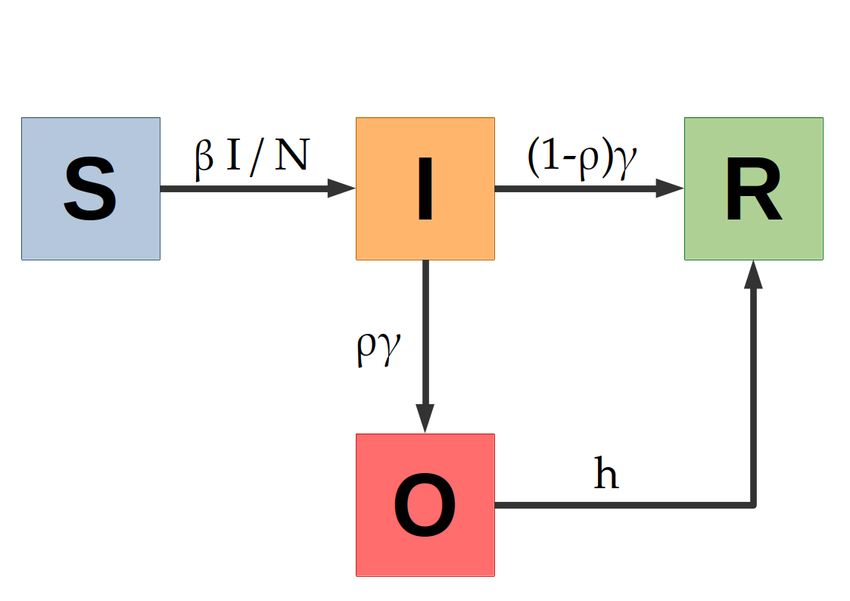
The model relies on four compartments, namely: S, I, O, R. Hence, S(usceptible)
individuals can become I(nfective) when meeting another infective individual,
I(nfectives) either become O(bserved) – i.e. present symptoms acute enough to
be detected from the national health-care system – or are R(emoved) from the
infection cycle by having recovered; also O(bserved) individuals are eventually
R(emoved) from the infection cycle2 . In the case of Covid-19, it is not clear yet
if there is an asymptomatic phase [16, 17]; in the model, we implicitly assume
that asymptomatics are infective and their removal time is the same of the I
2 We are implicitly absorbing the number of deaths in the R(emoved) compartment of the
model, that therefore comprises both the Recovered people (who hopefully have developed
antibodies and are not anymore susceptible) and the small fraction of those who did not
overcome the epidemics
3class. The model is described by the following differential equations:
I
∂t S = −βS
N
I
∂t I = βS − γI (1)
N
∂t O = ργI − hO
∂t R = (1 − ρ)γI + hO
N = S + I + O + R is the total number of individuals in a population, the
transmission coefficient β is the rate at which a susceptible becomes infected
upon meeting an infected individual, γ is the rate at which an infected either
becomes observable or is removed from the infection cycle. Like the SIR model,
the basic reproduction number is R0 = β/γ; the extra parameters of the SIOR
model are ρ, the fraction of infected that become observed from the national
health-care system, and h, the rate at which observed individuals are removed
from the infection cycle. Notice that we consider that O(bserved) individuals
not infecting others, being in a strict quarantine.
3 The Italian Lockdown
The Italian lockdown measures of the 8th and 9th of March [18, 19] aimed to
change mobility patterns and to reduce the intensity of social contacts, through
quarantine measures and to an increased awareness of the importance of social
distancing. We analyze an extensive data set on Facebook mobility data3 [20];
our analysis confirms that the lockdown has reduced both the travelled distance
and the flow of travelling people.
We consider the effects of lockdown measures on the parameters of our model.
Lockdown is a non-pharmaceutical measure; hence the rate γ is the most unaf-
fected parameter, since it is related to the “medical” evolution of the disease.
Analogous arguments apply to the rate h of exiting a condition serious enough to
be observed and to the probability ρ of being observed by the national healthcare
system (although ρ could be influenced variations in testing schemes and alert
thresholds). On the other hand, the transmission coefficient β can be thought
as the product Cλ of a contact rate C times a disease-dependent transmission
probability λ. Hence, if we assume that the speed of Covid-19 mutation is ir-
relevant on our timescales, lockdown strategies mostly influence β by reducing
the contact rate C between individuals.
To adapt the SIOR’s parameters to the Italian data [21], we compare the
reported cumulative number of Covid-19 cases Y Obs with the analogous quantity
model
R
Y = ργIdt in our model. We want to stress that our model fitting is not
aimed to produce an accurate model for detailed predictions, but to work in a
realistic region of the parameter space.
3 Those data are part of the Facebook project “Data for Good”, and illustrate mo-
bility patterns of fb users, who allowed the social network to track their location. See
https://dataforgood.fb.com/docs/Covid-19/
4We first estimate model’s parameters by least square fitting on the pre-
lockdown period. Since in such range the data Y Obs show an exponential growth
trend, we are possibly observing a very early phase of the epidemic, where β − γ
equals the growth rate of Y Obs (see APPENDIX for observations on the choices
of initial parameters). For fixed β − γ, the time of the epidemic start (that we
conventionally assume as the time t0 where the number of infected is 1) and the
fraction ρ of serious cases observed by the national healthcare service, allows to
vary the values of β and γ as long as their difference is fixed. Hence, estimating
medical parameters as the rate γ of escaping the infected state is paramount for
calibrating mathematical models.
In response to the outbreak of Covid-19, several estimates of model param-
eters have been proposed in the literature, revealing a certain amount of uncer-
tainty about some fundamental variables of the epidemic contagion. The Euro-
pean Centre for Disease controls reports an infection time duration τI between 5
and 14 days [22]; in our model, we will use τI = 10 (i.e. γ = τI−1 = 1/10 days−1 ).
According to a report of ISS, the Italian National Health Institute, the time from
the start of serious symptoms (i.e. when one gets “observed” from ISS) to the
resolution of the symptoms can be estimated as τH ∼ 9 days [23], correspond-
ing in our model to a value h = 1/9 days−1 . Notice the analysis of 12 different
models [13] reports varying estimates for the basic reproduction number R0 ,
ranging from 1.5 to 6.47, with mean 3.28 and a median of 2.79.
From fitting the 15 days of Y obs (pre-lockdown phase) and by performing a
bootstrap sensitivity analysis of the parameters, we obtain β − γ ∼ 0.25 ± 0.01
and t0 = −30 ± 5 days by assuming that ρ = 40%. Varying ρ in [10%, 100%]
varies β − γ in [0.22, 0.27]. On the other hand, for fixed β − γ, R0 would
vary linearly with τI ; as an example, R0 varies in [2.5, 4.5] for the literature
parameters τI ∈ [5, 14]; accordingly, to adjust the difference in growth rate, t0
varies in [26, 32]. However, despite the variability of the parameter range, the
qualitative behavior of the model – and hence our analysis of the key factors of
the epidemic evolution – is unchanged.
We then assume that, after the lockdown day tLock = 15 (corresponding to
the 9th of march), contact rate drops down by a factor α and hence β → αβ.
By fitting the observed data Y obs for a symmetric period of 15 days after tLock ,
and by performing a bootstrap sensitivity analysis, we find α = 0.49 ± 0.01, i.e.
a ∼ 50% reduction in infectivity and hence in R0 . Our figure is in line with
the observed reduction in R0 in response to the combined non-pharmaceutical
interventions, that across several countries has and average reduction of 64%
compared to the pre-intervention values [24]. Notice that Facebook mobility
data show a post-lockdown reduction in mobility of 15% at regional level and of
73% at inter-regional level; however, as we will point out later, mobility has a
strong impact at the beginning of the epidemics in new regions/countries, while
it has much lower effects on the evolution of the epidemics in a region/country.
In the following, we will use the parameters of Tab. 1, corresponding to a
basic reproduction number R0 = 3.5. Moreover, since patients in intensive care
represent the highest burden for health facilities, in the graphs of the paper we
will indicate the number of patients in intensive care, estimated as 3.5% of the
5β = 0.35 day −1 γ = 10−1 day −1 h = 1/9 day −1
t0 = −30 days ρ = 40% α = 0.49
Tab. 1. Standard parameters used for the SIOR model in the paper.
total patients by using the figures reported by ISS [21].
4 National scenarios and exit mechanisms
Since we are interested on the factors driving the exit dynamics from lock-
down, and not on the detailed analysis of realistic scenarios, we consider several
lockdown scenarios, where the lockdown is abruptly lifted and the system let
return to the pre-lockdown parameters. Such an approach clearly describes a
worst-case estimate of the intensity of the second wave of the contagion after
the conclusion of the lockdown. Hence, we consider several simplified scenarios,
where we use the SIOR model described by System 2 with the parameters of
Tab. 1. First, in the simple case of a SIOR model fitted on Italian data, we
analyze how the post-lockdown dynamics changes according to different starting
dates of the epidemics and to different levels of the restrictions implemented by
the national authorities. Then, we study the effect of explicitly considering Italy
as a collection of separate administrative entities (Regions); finally, we consider
the effects of social interactions across age class.
Interestingly, mobility flows [20] and inter-age social mixing [25] lie at the two
opposite range of modelling. In fact, the regional social contact matrix is dense
(Fig. 1, left panel), indicating that age classes dynamics are strongly coupled.
On the other hand, the inter-regional mobility matrix is very sparse (Fig. 1,
right panel), indicating that regions have their own independent dynamics.
We first consider a simple exit strategy consisting in lifting the lockdown at
a time tUnlock after the peak of O has occurred. For instance, we hypothesize
that infection proceeds uncontrolled up to time tLock ; in the following lockdown
period [tLock , tUnlock ], the transmission coefficient β is reduced by a factor α;
finally, β returns to its initial value and herd immunity is responsible for the
dampening of the epidemics.
Our results show that the lockdown lowers the peak of O - i.e. the indi-
viduals with noticeable symptoms - to ∼ 70% of the free epidemic one, but it
also doubles the time of its occurrence from ∼ 1.9 months to ∼ 3.8 months:
an extremely obnoxious effect for the sustainability conditions of the economy
of a country. However, since the number of hospitalized patients and - most
importantly - the number of patients in intensive care is only a fraction of O,
lowering the peak puts less stress on the healthcare system. The ideal situation
would be to have accurate data, an accurate model and accurate estimates of
the parameters; as an example, in our model lifting the lockdown when the
number of infected people per unit time βS(t)I(t)/N is lower that the average
number of recovering people γI(t) would ensure that the number of infections
6Fig. 1. Left Panel: social contact matrix, from [25]. Right panel: inter-regional
mobility matrix, from the Facebook project “Data for Good”. The intensity of
a color maps the strength of a matrix element (light colors: high values; dark
colors: low values). The inter-age social mixing matrix is dense; hence age
classes dynamics are strongly coupled. The inter-regional mobility flows is very
sparse (i.e. off diagonal elements are order of magnitudes lower than diagonal
elements): this mean that most of the people travel within the same region of
origin; hence, the regional dynamics can be considered “almost” decoupled.
would continue to decrease. In real life, situations are more fuzzy: having not
enough information, we could decide to resort on some heuristics, like lifting the
lockdown after the observed people O have dropped to a suitable percentage of
the maximum peak. As an example, after ∼ 4.7 months the peak has reduced
to 70% of its initial value, while after ∼ 5.2 months to 50%, i.e. ∼ 0.5 months
later. Notice that, the earlier the lockdown is lifted, the faster O decays to zero
even if it starts from higher figures and could even experience a rebound. All
such effects are shown in Fig. 2.
Our framework sustains the identification of several mechanisms. The first is
related to the timeliness of the lockdown, i.e. to the choice of anticipating tLock .
As expected, early lockdown (i.e. well before the “free” infection peak) reduces
the height of the peak without much moving it forward in time. Conversely,
lifting the lockdown too soon can make epidemic start again and reach values
higher than the ones before the release. A peculiar and counter-intuitive effect
can be generated if the lockdown is anticipated: in fact, a too early lockdown de-
lays the start of the epidemic without attenuating its severity (see APPENDIX
for the description of the effects of varying lockdown time). In other words, an
early lockdown “buys” time, but it postpones the problem without mitigating
its severity.
Another effect is the impact of extreme social and physical distancing mea-
sures on the post-lockdown dynamics. Increasing the strength α of the lockdown,
not only corresponds to delaying the time at which it is lifted, but it also induces
a stronger re-start of the epidemic in the post-lockdown (see APPENDIX for
7Fig. 2. Comparison of the scenarios where the lockdown is relaxed after the
percentage of people with visible symptoms (O) is reached the 70% and the
50% of the reported cases peak. Lifting the lockdown earlier has the epidemics
disappear faster, but has higher impact on the number of hospitalized and in-
tensive care patients; moreover, lifting the lockdown too early can result in a
rebound of the number of cases.
the description of the effects of varying lockdown strength), triggering a new
lockdown. Such scenario would obviously be unsustainable, in terms of social
and economic costs.
An additional counter-intuitive mechanism must be considered. Since an at-
tenuation of α corresponds to an effective reproduction number R0eff = αR0 , at
the critical value αcrit = 1/R0 the epidemic neither grows nor decreases4 . Thus,
after tLock the system stays stationary until the lockdown is released at tUnlock ;
at this point, the epidemic starts growing again as it was before the lockdown.
In general, if α < αcrit , the system looks to ameliorate (infected, hospitalized,
all the infective compartments go down) but as soon as the lockdown is lifted,
the epidemic starts again to reach its full strength (see SI). Nevertheless, our
estimate α ∼ 0.5 > αcrit ∼ 0.3 for the Italian lockdown gives us hope that,
perhaps, it will not be necessary to follow a repeated seek-and-release strategy
in the post-lockdown phase. On the other hand, if it can be attained a lock-
down strength α ∼ αcrit without disrupting the economy, the epidemic could be
contained until the creation, production and distribution of a vaccine.
5 Regional Scenarios
Starting with the first confirmed cases in Lombardy on 21 February, by the
beginning of March the Covid-19 outbreak had already spread to all italian
regions. While the delay in the beginning of the infection is accounted for by the
4 To be precise, the decrease becomes sub-exponential, thus taking a practically infinite
time when the size of the population is large
8Tab. 2. Regional delays (in days)
Lombardia 0.0 Molise 10.6
Emilia Romagna 3.1 Umbria 11.8
Marche 4.3 Abruzzo 13.1
Veneto 5.7 Lazio 14.5
Valle d’Aosta 6.4 Campania 15.0
P.A. Trento 6.6 Puglia 15.7
P.A. Bolzano 8.0 Sardegna 16.2
Liguria 8.1 Sicilia 16.6
Friuli Venezia Giulia 8.9 Calabria 17.2
Piemonte 9.0 Basilicata 19.2
Toscana 10.4
different mobility interaction between regions, once the epidemic has started in a
given area, the intake of external infected people becomes quickly irrelevant (see
APPENDIX for the description of a metaregional model and its behavior). As a
consequence, the growth curves of the epidemic variables tend to converge to the
same shape (see APPENDIX about using normalised data). In fact, regional
info graphics released by the Italian National Healthcare Institute (ISS) [21]
show that regional diffusion curves have a similar shape and different starting
dates (see Fig. 3). This observation can be justified as follows: Italian regions are
independent administrative entities, and most of the population tend to work
inside the resident region [26]. Hence, epidemics propagate from region to region
via the fewer inter-regional exchanges (Incidentally, Lombardy is the Italian
region, which is most involved in international trade connections [27], being the
natural candidate for the initial outbreak of the epidemic). More practically, we
estimate the delays by minimizing the distance among the observed curves (see
APPENDIX for the details of the algorithm); results are reported in Tab. 2.
Notice that, assuming Lombardy has been the first region (i.e. delay=0), the
resulting regional delays are mostly correlated to geographical distances.
We assume that the Covid-19 outbreak spreads independently in each region;
as argued before, such an approximation is reasonable after the epidemic has
started and is even more accurate under lockdown conditions. Hence, we apply
the parameters for the entire country to regional cases5 , where now the maxi-
mum number of individuals Ni is the population of the ith region6 . Then, by
summing up all the Si , . . . , Ri , respectively, we obtain a proxy for the global evo-
lution of Covid-19 epidemic throughout Italy. To evaluate the effect of Phetero-
geneity in time delays, we compare the number of daily cases ODelay = OiDelay
(obtained by taking into account the regional delays ti as reported in Tab. 2)
5 Again, we are exploring qualitative scenarios and we do not aim to predict the real evolu-
tion of the epidemics: in fact, Italian regions are different for social contact habits, mobility,
organization and capacity of health care provision, as well for factors that affect the medical
parameters, like comorbidities, social conditions or pollution levels.
6 https://www.istat.it/it/popolazione-e-famiglie?dati
9with the number of daily cases O0 = Oi0 we would observe by considering the
P
epidemics starts at the same time t0 in all regions. As expected, heterogeneity
flattens the curve and shifts its maximum later in time. This is a first source of
errors when fitting an heterogeneous dynamics with a global model.
We do take into account regional delays and consider two possible exit strate-
gies: in the first, that we call the Asynchronous scenario, each region i lifts the
lockdown at the time tUnlock
i when the peak of OiDelay decreases by 30%; in the
second, that we call the Synchronous scenario, each region i lifts the lockdown
at the same time tUnlock , i.e., when the global peak of ODelay decreases by 30%.
The choice of 30% is arbitrary, similar results would hold for choices of values
near the peak; it tries to be a sketch of a situation where, due to economic
pressure, lockdown is lifted as soon as possible.
Notice that, once an outbreak has started, the epidemic dynamics in a given
region i is essentially uncorrelated with the epidemic spreading of any other
region j 6= i. Therefore, it could be safe and appropriate to decide the lockdown
lifting time on a regional basis, instead of lifting restrictions throughout Italy
at the same time. Indeed, it could be unreasonable to keep locked the regions
where the epidemic started earlier; on the contrary, regions where the epidemic
began with some delay could experience a strong rebound when subjected to a
premature lockdown lifting. In Fig. 3 we show the effects of lifting the lockdown
at both regional (Async) and national (Sync) level in Lazio and Lombardy. Since
not only epidemics, but also the ruin of an economy is a non-linear process, the
Sync scenario can turn out to be even more disruptive than the epidemic itself
(see also Fig. 2). Notice that analogous arguments hold - mutatis mutandis -
also for the world/countries scenario.
6 The role of Age
As we have already observed in the previous Section, heterogeneity strongly im-
pacts on the results within the model [28]. Since the transmission coefficient is
proportional to the contact rate between individuals, the rates of social mixing
between different age classes represent a well known important source of het-
erogeneity. This information can estimated either through large-scales surveys
[25] or through virtual populations modeling [29]. While the POLYMOD [25]
matrices have been extensively used to estimate the cost-effectiveness of vacci-
nation for different age-classes during the 2009 H1N1 pandemic [30, 31], here
they are used to support the design of a broad class of exit strategies. Hence,
to account for age classes, we extend our model by rewriting the transmission
coefficient as βC (see APPENDIX for a full description of the extended model),
where β is the transmission probability of the infection, and C is the sociological
matrix describing the contact patterns typical of a given country. For lack of
further information, we assume β constant among age classes and C as in [25].
To simplify the analysis, we gather POLYMOD age groups into three classes:
Y oung (00 − 19), M iddle (20 − 69) and Elderly (70+) (see Tab 3). Such an
aggregation puts together the most “contactful” classes (00 − 19), the classes
10Fig. 3. Upper panels: analysis of time delays among the start of epidemics in
11
different regions (see Tab. 2). Lower panels: sketch of an Async(hronous) exit
strategy (i.e. each region lifts the lockdown following its own policy) respect to
a Sync(hronous) exit strategy (i.e. the lockdown lift follows the same policy,
but applied to a nation wide scale). In particular, tSync corresponds to lifting
the lockdown in all the region after the peak has fallen by 30% , while tAsynci
corresponds to lifting the lockdown in the ith region after the peak of such region
has fallen by 30%.Y M E
Y 2.35 0.44 0.67
M 0.47 0.59 0.50
E 0.50 0.55 0.80
Tab. 3. POLYMOD matrix aggregated for three age classes: Y oung (00 − 19),
M iddle (20 − 69) and Elderly (70+).
Fig. 4. Comparison of the scenarios where the lockdown is relaxed only for
a particular age class with respect to a full release policy. Strategies: YE =
quarantine young and elderly, E = quarantine elderly. Notice that we have pur-
posefully left the M class fully unrestrained, in order to show how maintaining
a partial, age-based lockdown could deeply change the effectiveness of the exit
strategy.
with the highest mortality risk (70+) [21], and a good approximation of the
active population (20 − 69).
Fig. 4 shows how the percentage of people with visible symptoms (O) varies
once the age class heterogeneity is considered in the model. Differently from fig.
2, fully lifting the lockdown results in a conspicuous rebound of the epidemics,
that reaches values even more severe than the pre-exit peak. Thus, models,
which do not explicitly consider this source of heterogeneity could severely mis-
forecast the post-exit dynamics. On the other hand, the introduction of the
age structure in the model allows to orient the design of exit strategies based on
age-targeted policies, as a way to dampen a possible upturn of contagion. Specif-
ically, social/physical distance measures applied to the elderly may contribute
to contain the impact of a renewed upward phase, while relaxing restrictions
to the working age class (20-69) would not impair the smoothing of contagion
propagation in the post-lockdown phase. Again, a disclaimer, it is important to
emphasize that we are referring to simple mock-up strategies, which correspond
to worst-case scenarios: in real life, community measures and physical distanc-
ing, infection prevention and control, personal hygiene habits, face mask usage,
12etc. will be decisive in contributing to the dampening of the epidemics [22].
7 Conclusions
In this paper we propose and test a general framework to study the Covid-19
contagion through a compartmental model, with a focus on geographical groups
and age classes. Our framework shows that the promptness of lockdown mea-
sures has a main effect on the timing of the contagion. Strict social distancing
policies reduce the severity of the epidemics during the lockdown period, but
full recover of the contagion can occur once such measures are relaxed. As a
consequence, a mix of specific mitigation strategies must be prepared during
the lockdown and implemented thereafter. In order to understand the relative
potential impact of different broad strategies, we focus on two broad decom-
position criteria within the model, that is geographical mobility and social in-
teractions between age classs. Our results are driven by the sparsity of the
underlying contact matrices, which we measure. First, we show how local dy-
namics at regional level can be hidden when observing the aggregate national
system. Regional heterogeneity tends to lower and widen the curve of the con-
tagion, contributing to a shift forward in time for the peak at the aggregate
level. Moreover, our analysis of mobility data shows that, due to the sparsity of
interconnections across regions, contagion develops independently within each
region once the epidemic has started. This, in turn, contributes to account for
the delays observed in the alignment of the contagion curves across different
geographical areas. The independence of regional dynamics is important, since
it can justify the adoption of a mix between general mitigation strategies and
solutions which are specific to individual regions or to clusters of regions. In-
terestingly enough, the generality of our model makes this result relevant also
to frame the relative impact of cross country mobility flows. Finally, we inves-
tigate the structure of social contacts across different settings and we quantify
the relative importance of interactions between age classes in the spreading of
contagion. We show that the young (0-19) and the old (70+) are the most
intensively interacting classes. As a consequence, mitigation strategies specific
to these two classs can produce a significant impact on diffusion rates in the
post-lockdown phase. In fact, our results show the importance of designing
physical distancing measures specific to the elderly and, in addition, they can
orient decisions on limitations to social contacts for the young. Overall, our
results provide guidance on how to relax some of the restrictions to mobility for
the active population (20-69), while smoothing and lessening the propagation
of contagion in the post-lockdown phase.
Although our study is tuned on the Italian Covid-19 contagion, our modeling
approach is general enough to help us understand the role of relevant dimen-
sions, beside the medical and pharmaceutical ones, in identifying the relative
importance of different strategies introduced to contain the epidemics and to
mitigate its effects. Our framework can contribute to mitigate the stringency
of the trade-off between health and economic outcomes. In particular, we show
13how the timeline of post-lockdown measures should take into account some fun-
damental compartmental aspects, such as geographical factors and interactions
between different age classes. This feature is general, and it can orient the
analysis towards fine grained simulations on the impact of specific precaution-
ary interventions, which enforce social distancing while containing the overall
burden on the economy and on society.
References
[1] Matt J Keeling. Models of foot-and-mouth disease. Proceedings of the
Royal Society B: Biological Sciences, 272(1569):1195–1202, 2005.
[2] Francesco Di Lauro, István Z Kiss, and Joel Miller. The timing of one-shot
interventions for epidemic control. medRxiv, 2020.
[3] Vital Surveillances. The epidemiological characteristics of an outbreak
of 2019 novel coronavirus diseases (covid-19)—china, 2020. China CDC
Weekly, 2(8):113–122, 2020.
[4] Roy M Anderson, Hans Heesterbeek, Don Klinkenberg, and T Déirdre
Hollingsworth. How will country-based mitigation measures influence the
course of the covid-19 epidemic? The Lancet, 395(10228):931–934, 2020.
[5] Herbert A Simon and Albert Ando. Aggregation of variables in dynamic
systems. Econometrica: journal of the Econometric Society, pages 111–138,
1961.
[6] Albert Ando and Franklin M Fisher. Near-decomposability, partition and
aggregation, and the relevance of stability discussions. International Eco-
nomic Review, 4(1):53–67, 1963.
[7] Herbert A Simon. The architecture of complexity. Cambridge, MA: MIT
Press, 1996.
[8] Pierre Jacques Courtois. Decomposability: queueing and computer system
applications. Academic Press, 2014.
[9] Neil Ferguson, Daniel Laydon, Gemma Nedjati Gilani, Natsuko Imai, Kylie
Ainslie, Marc Baguelin, Sangeeta Bhatia, Adhiratha Boonyasiri, ZULMA
Cucunuba Perez, Gina Cuomo-Dannenburg, et al. Report 9: Impact of
non-pharmaceutical interventions (npis) to reduce covid19 mortality and
healthcare demand. MRC Centre for Global Infectious Disease Analysis,
2020.
[10] Kiesha Prem, Yang Liu, Timothy W Russell, Adam J Kucharski, Ros-
alind M Eggo, Nicholas Davies, Stefan Flasche, Samuel Clifford, Carl AB
Pearson, James D Munday, et al. The effect of control strategies to reduce
social mixing on outcomes of the covid-19 epidemic in wuhan, china: a
modelling study. The Lancet Public Health, 2020.
14[11] Matteo Chinazzi, Jessica T Davis, Marco Ajelli, Corrado Gioannini, Maria
Litvinova, Stefano Merler, Ana Pastore y Piontti, Kunpeng Mu, Luca Rossi,
Kaiyuan Sun, et al. The effect of travel restrictions on the spread of the
2019 novel coronavirus (covid-19) outbreak. Science, 2020.
[12] Norman TJ Bailey et al. The mathematical theory of infectious diseases
and its applications. Charles Griffin & Company Ltd, 5a Crendon Street,
High Wycombe, Bucks HP13 6LE., 1975.
[13] Ying Liu, Albert A Gayle, Annelies Wilder-Smith, and Joacim Rocklöv.
The reproductive number of covid-19 is higher compared to sars coron-
avirus. Journal of travel medicine, 2020.
[14] Francesco Casella. Can the covid-19 epidemic be managed on the basis of
daily data? arXiv preprint arXiv:2003.06967, 2020.
[15] Sebastian Funk, Marcel Salathé, and Vincent AA Jansen. Modelling the
influence of human behaviour on the spread of infectious diseases: a review.
Journal of the Royal Society Interface, 7(50):1247–1256, 2010.
[16] Yan Bai, Lingsheng Yao, Tao Wei, Fei Tian, Dong-Yan Jin, Lijuan Chen,
and Meiyun Wang. Presumed asymptomatic carrier transmission of covid-
19. Jama, 2020.
[17] Hiroshi Nishiura, Tetsuro Kobayashi, Takeshi Miyama, Ayako Suzuki,
Sungmok Jung, Katsuma Hayashi, Ryo Kinoshita, Yichi Yang, Baoyin
Yuan, Andrei R Akhmetzhanov, et al. Estimation of the asymptomatic
ratio of novel coronavirus infections (covid-19). medRxiv, 2020.
[18] Decreto del Presidente del Consiglio dei Ministri. Ulteriori disposizioni
attuative del decreto-legge 23 febbraio 2020, n. 6, recante misure urgenti
in materia di contenimento e gestione dell’emergenza epidemiologica da
covid-19. Gazzetta Ufficiale, 59(08-03-2020), 2020.
[19] Decreto del Presidente del Consiglio dei Ministri. Ulteriori disposizioni
attuative del decreto-legge 23 febbraio 2020, n. 6, recante misure urgenti
in materia di contenimento e gestione dell’emergenza epidemiologica da
covid-19. Gazzetta Ufficiale, 62(09-03-2020), 2020.
[20] Caroline O Buckee, Satchit Balsari, Jennifer Chan, Mercè Crosas,
Francesca Dominici, Urs Gasser, Yonatan H Grad, Bryan Grenfell, M Eliz-
abeth Halloran, Moritz UG Kraemer, et al. Aggregated mobility data could
help fight covid-19. Science (New York, NY), 2020.
[21] Istituto Superiore di Sanità. Iss: Sars-cov-2 dati epidemiologici (https:
//www.epicentro.iss.it/). Technical report, ISS, 2020.
[22] European Centre for Disease Prevention and Control (ECDC). Coronavirus
disease 2019 (covid-19) pandemic: increased transmission in the eu/eea and
the uk – eigth update, 8 april 2020. 2020.
15[23] Istituto Superiore di Sanitá (ISS) COVID-19 Surveillance Group. Charac-
teristics of covid-19 patients dying in italy report based on available data
on march 30th, 2020. 2020.
[24] Seth Flaxman, Swapnil Mishra, Axel Gandy, H Unwin, H Coupland, T Mel-
lan, H Zhu, T Berah, J Eaton, P Perez Guzman, et al. Report 13: Esti-
mating the number of infections and the impact of non-pharmaceutical
interventions on covid-19 in 11 european countries. 2020.
[25] Joël Mossong, Niel Hens, Mark Jit, Philippe Beutels, Kari Auranen, Rafael
Mikolajczyk, Marco Massari, Stefania Salmaso, Gianpaolo Scalia Tomba,
Jacco Wallinga, et al. Social contacts and mixing patterns relevant to the
spread of infectious diseases. PLoS medicine, 5(3), 2008.
[26] Istituto Nazionale di Statistica. Popolazione insistente per
studio e lavoro (https://www.istat.it/it/files//2020/03/
Popolazione-insistente.pdf). Technical report, ISTAT, 2020.
[27] Istituto Nazionale di Statistica. Commercio estero (https://www.istat.
it/it/commercio-estero). Technical report, ISTAT, 2020.
[28] Odo Diekmann, Johan Andre Peter Heesterbeek, and Johan AJ Metz. On
the definition and the computation of the basic reproduction ratio r 0 in
models for infectious diseases in heterogeneous populations. Journal of
mathematical biology, 28(4):365–382, 1990.
[29] Laura Fumanelli, Marco Ajelli, Piero Manfredi, Alessandro Vespignani, and
Stefano Merler. Inferring the structure of social contacts from demographic
data in the analysis of infectious diseases spread. PLoS computational
biology, 8(9), 2012.
[30] Jan Medlock and Alison P Galvani. Optimizing influenza vaccine distribu-
tion. Science, 325(5948):1705–1708, 2009.
[31] Marc Baguelin, Albert Jan Van Hoek, Mark Jit, Stefan Flasche, Pe-
ter J White, and W John Edmunds. Vaccination against pandemic in-
fluenza a/h1n1v in england: a real-time economic evaluation. Vaccine,
28(12):2370–2384, 2010.
[32] Lars Hufnagel, Dirk Brockmann, and Theo Geisel. Forecast and control of
epidemics in a globalized world. Proceedings of the National Academy of
Sciences, 101(42):15124–15129, 2004.
[33] Roger Guimera, Stefano Mossa, Adrian Turtschi, and LA Nunes Amaral.
The worldwide air transportation network: Anomalous centrality, commu-
nity structure, and cities’ global roles. Proceedings of the National Academy
of Sciences, 102(22):7794–7799, 2005.
16[34] IM Hall, JR Egan, I Barrass, R Gani, and S Leach. Comparison of smallpox
outbreak control strategies using a spatial metapopulation model. Epidemi-
ology & Infection, 135(7):1133–1144, 2007.
[35] Cécile Viboud, Ottar N Bjørnstad, David L Smith, Lone Simonsen, Mark A
Miller, and Bryan T Grenfell. Synchrony, waves, and spatial hierarchies in
the spread of influenza. science, 312(5772):447–451, 2006.
178 APPENDIX
In Sec. 8.1 we describe the SIOR model used in the paper, stressing the general
problems related to fitting real data with compartmental models. In Sec. 8.2
we discuss the effects of varying the starting date and the strength of the lock-
down measures. The algorithm used for finding delays among growth curves
is described in Sec. 8.3, whereas the reasons why classic growth curves could
have the same shape when normalised is discussed in Sec. 9. Moreover, Sec.
9.1 explicates why from an extension of a simple compartmental model to a
regional metapopulation model with a very low mobility among regions it is to
be expected that regions show similar dynamics like in Sec. 9 but shifted in
time. Finally, Sec. 9.2 shows the extension of a simple compartmental model
to consider social mixing among different age classes.
8.1 Basic model
Our model belongs to the classic family of compartmental models [12]. As
the most renewed SIR and SEIR model (and their variations), it models the
infection rate to be proportional to the number of individuals in a S(usceptible)
compartment (i.e., the ones that have never been infected) times the probability
of meeting infected persons (modelled as the fraction I/N of individuals in the
I(nfectious) compartment respect to the population size N ). The other essential
rate is represented by individuals that are Removed (either because recovered
and not more susceptible, or because deceased) from the I class; again, such
rate is proportional to the number of individuals in I. To have the possibility of
adjusting our model’s parameter with the observed data, we introduce another
class O of “observable” people, i.e. people with symptoms strong enough to be
detected by the national healthcare system. A graphical sketch of the model is
presented in fig.5.
The SIOR model is described by the following set of ordinary differential
equations:
I
∂t S = −βS
N
I
∂t I = βS − γI (2)
N
∂t O = ργI − hO
∂t R = (1 − ρ)γI + hO
where N = S + I + O + R is the total number of individuals in a population, the
transmission coefficient β is the rate at which a susceptible becomes infected
upon meeting an infected individual, γ is the rate at which an infected either
becomes observable or is removed from the infection cycle. The extra parameters
of the model are ρ, the fraction of infected that become observed from the
national health-care system, and h, the rate at which observed individuals are
removed from the infection cycle. Notice that we consider that O(bserved)
individuals not infecting others, being in a strict quarantine.
18Fig. 5. The SIOR compartmental model: workflow of the epidemic process. A
S(usceptible) individual becomes I(nfectious) when meeting an infected person.
An I(nfectious) either become O(bserved), with symptoms acute enough to be
detected from the national health-care system, or is R(emoved) from the infec-
tion cycle by having recovered. An O(bserved) individual can also be R(emoved)
from the infection cycle having become immune. The parameter β defines the
rate at which a susceptible becomes infectious, γ represents the rate at which
infectious either become observable or recover, ρ is the fraction of infectious
that become observed from the national health-care system and h is the rate at
which observed individuals are removed from the infection cycle.
19As for the SIR model, the basic reproduction number can be calculated as
R0 = β/γ and the stationary state can be estimate as follows. Let us consider
X = O +R, it holds ∂X S = −R0 S and S(t → ∞) = N e−R0 X(t→∞) . Then, since
O(t → ∞) = I(t → ∞) = 0, it follows that R(t → ∞) = N − S(t → ∞) and we
recover the same solution of the SIR model: S(t → ∞) = N e−R0 [N −S(→∞)] .
8.1.1 Initial parameters estimation
In the early phases of the epidemic, the observed quantities follow an approxi-
mately exponential growth Y Obs ∼ Y0 egt , as expected in most epidemic models.
To understand what happens in our model, we notice that for I/S
1 we can
linearize System 2 resulting in I ∼ I0 e(β−γ)t and O ∼ ργI. Thus, minimizing
the difference between O and Y Obs in the early period would yield estimates for
β, γ such that β − γ ∼ g, and R0 ∼ 1 + g/γ would increase linearly with the
characteristic time τI = γ −1 for exiting the infectious phase. Notice that most
of the compartmental models based on a set of ordinary differential equations
show an initial exponential growth phase with the same exponent (see Fig. 6);
hence, in the early stage of the epidemic it is possible to successfully fit the
“wrong” variables.
8.2 Effects of lockdown time and strength
By increasing the strength α of the lockdown (where α is the ratio between
the trasmission β after and before the lockdown) the epidemic peak is pushed
forward, but the height of it is lower. On the other hand, the epidemic delaying
implies that lifting the lockdown would bring back the infection. In the left
panel of Fig. 7, we show what happens by lifting the lockdown when the peak
is fallen by 30%: stronger lockdowns induce a stronger reprise of the epidemic.
An analogous effect can be observed by varying the lockdown time: anticipating
the lockdown ameliorates the peak by decreasing its height, but shifts it to later
time and retards the end of the epidemic.
Contrary to what could be naively expected, an early imposition of the
lockdown does not ameliorate the epidemics: in fact, anticipating too much the
lockdown just shifts the timing of the epidemics, leaving its evolution unchanged
(see Fig. 8). This is to be expected every time extreme measures of social
distancing are applied in the very early, exponentially growing, stages. In fact,
let us consider two countries A and B that have the same population, the same
contact matrix, and the same number of infected persons. If A and B decide
to put a lockdown of strength α at time tA and tB , respectively, at time t any
quantity y of the model would have grown as yA (t) ∼ y 0 eR0 tA eαR0 (t−tA ) and
as yB (t) ∼ y 0 eR0 tB eαR0 (t−tB) . If there exists a t0 such that yA (t) = yB (t0 ),
the epidemics in A and in B will proceed in parallel (even in the non-linear
phase) with a delay t0 − t. Therefore, if the epidemic dynamics of A and B
are still well approximated by exponential distributions at times < max{t, t0 },
then t0 − t ∝ −(tA − tB ), i.e, the country that has started the lockdown before
will experience the same epidemic of the other country, just delayed in time. In
20Fig. 6. In the initial stage, most of the quantities experience an exponential
growth with the same exponent; hence, it would be possibly to “successfully”
fit the wrong variables. Figure shows the pre-lockdown growth of the number
of I(nfected), O(bserved), R(emoved) individuals in our model (2). Full circles
represent the experimental counts of confirmed Covid-19 cases in Italy; X is the
cumulative variable we use to fit the experimental data.
21Fig. 7. Left panel: variation of the behavior of the model by varying the
lockdown strength α. Lockdown starts at tLock = 15 and is fully lifted when the
peak has fallen by 30%. Right panel: variation of the behavior of the model by
delaying the lockdown time tLock . Lockdown strength is fixed at α = 0.5 and is
fully lifted when the peak has fallen by 30%.
22Fig. 8. Upper panel: variation of the behavior of the model by anticipating
the lockdown time. Notice that anticipating the lockdown leaves unchanged the
behaviour of the epidemics, just shifting all the times of an amount proportional
to how much the lockdown is anticipated. Lockdown strength is fixed at α = 0.5
and is fully lifted when the peak has fallen by 30%. Lower panel: by applying
the Eq. 3, we show how the curves in the upper panel collapse on each other.
particular, for identical initial conditions, we have that:
1+α
t − t0 = − (tA − tB ) (3)
α
as long as all the times are before the initial exponential regime ends. Such an
estimate can be very useful for countries where the epidemics has not started
yet. Indeed, calibrating on one own normalized growth curve the time of the
lockdown and its strength would give an idea of how long one can delay the full
start of the epidemic dynamics.
Finally, we notice that to each lockdown strength α corresponds an effective
reproduction number R0eff = αR0 ; hence, for α ∼ αcrit = 1/R0 , the epidemics
is expected to stay in a quiescent state where it does not either grow or decay
sensibly. On the other hand, for α < αcrit the epidemics decreases; nevertheless,
since this happens before a sufficient number of recovered individuals has built
up herd-immunization, the height of the peaks after the lockdown lifting are
almost unchanged if compared with the no lockdown scenario. Again, a “too
23Fig. 9. Upper panel: variation of the behavior of the model for lockdown
strengths α < αcrit = 1/R0 . Notice that the height of the peaks after the
lockdown is released is almost unchanged if compared with the no lockdown
scenario. Lockdown time is fixed at tLock = 15 and is fully lifted when the peak
has fallen by 30%. Lower panel: for better clarity, the plot is also reported in
log-linear scale.
good” intervention risks to postpone the problem without attenuating it. Notice
that, if one applies lockdowns with α < αcrit , it could be necessary to switch
back and forth to lockdown to avoid the peak go beyond the capacity of a
national healthcare system (see Fig. 9).
8.3 Estimation of the experimental time delays
We first normalize the observed data by dividing the number of non-zero ob-
servations in a region for the population of the region. Let yi be the nor-
malized observations for the ith region. For each pair of regions i, j, we de-
fine the variation interval ∆ij = [minij , maxij ] that contains the maximum
number of points of both yi and yj , i.e. minij = max{min(yi ), min(yj )} and
maxij = min{max(yi ), max(yj )}. The delay tij between the epidemics start in
i and j, respectively, is calculated by minimizing the square norm of k(∆ij ∩
yi (t)) \ (∆ij ∩ yj (t − tij )k, where ∆ij ∩ y denotes the values of y falling in the
interval ∆ij . Denoting with Ti the times corresponding to the observation in
∆ij ∩ yi , it is easy to verify that tij = hTi i − hTj i, where hT i is the average value
of the times contained in T .
249 Equivalence of normalized curves
Eq. 2 referred to region k becomes:
∂t Sk = −βSk Ik /Nk
∂t Ik = βSk Ik /Nk − γIk
(4)
∂t Ok = ργIk − hOk
∂t Rk = (1 − ρ)γIk + hOk
where Nk is the population of the region. By rewriting Eq. 4 in terms of nor-
malized quantities sk = Sk /Nk , . . . sk = Sk /Nk , we obtain the same equation
for all the regions:
∂t s = −βs i
∂t i = βs i − γi
(5)
∂t o = ργi − ho
∂t r = (1 − ρ)γi + ho
Hence, for similar initial conditions, by normalizing the experimental observa-
tions by the population, one should obtain similar time behaviors.
9.1 Regional metapopulation model
Let us assume that we know the fraction Tkl of people commuting from region
k to region l, Eq. 5 becomes:
X
∂t sk = −βsk Tkl il
l
X
∂t ik = βsk Tkl il − γ ik
(6)
l
∂t ok = ργ ik − h ok
∂t rk = (1 − ρ)γ ik + h ok
P
From mobility data, we know that k = l6=k Tkl /Tkk
1 and Tkk ∼ 1; in
particular, from Facebook mobility data we can estimate hk i ∼ 10−3 . If all the
neighbors of a given region k are fully infected (i.e. il = 1 ∀ l 6= k) and ik (t0 ) = 0,
then the variation of ik can be approximated as ∂t ik ∼ k +(β−γ) ik . Namely, as
soon as ik > k , ik will grow exponentially according to ∂t ik ∼ (β − γ) ik and k
will become irrelevant; that is to say, the dynamics of the regions will decouple.
P the other hand, if epidemic is decaying everywhere, then il
1 ∀ l 6= k; thus
On
l6=k Tkl il
k and equation again decouple, having each region followed Eq. 5
separately. In Tab. 4 we confront regions ordered by simulating an hypothetical
epidemics starting from Lombardy and propagating with Eq. 6, with regions
ordered by the estimated delays obtained by applied the algorithm of sec. 8.3.
It is reasonable to assume that inter-regional mobility has had a role in the
25Mobility Matrix Experimental Delays
Lombardia Lombardia
Emilia Romagna Emilia Romagna
Piemonte Marche
Veneto Veneto
Valle d’Aosta Valle d’Aosta
Trentino Alto Adige Liguria
Lazio Friuli Venezia Giulia
Liguria Piemonte
Toscana Trentino Alto Adige
Campania Toscana
Marche Molise
Friuli Venezia Giulia Umbria
Abruzzo Abruzzo
Umbria Lazio
Sardegna Campania
Sicilia Puglia
Molise Sardegna
Basilicata Sicilia
Puglia Calabria
Calabria Basilicata
Tab. 4. Region ordered by simulations using the mobility matrix (left column)
and by the delays obtained by rescaling experimental data (right column).
regional delay structure; however, many other factors come to play in the long
range propagation of epidemics: as an example, both airline transportation
network [32, 33] and individual work commutes [34, 35] have played important
roles in understanding the spread of infectious diseases.
9.2 Social mixing
To take account for social mixing, we rewrite the transmission coefficient as
the product of a transmission probability β times a contact matrix C whose
element Cab measure the average number of (physical) daily contacts among
an individual in class age a and an individual in class age b. Notice that the
probability that a susceptible in class a has a contact with an infected in class
b is the product of the contact rate Cab times the probability Ib /NB that in-
dividual in class b is infected. Hence, denoting with S a , . . . , Ra the number of
S(usceptibles),. . .,R(emoved) individuals in class age a, we can rewrite Eq. 2 as:
X Ib
∂t S a = −βS a Cab
Nb
b
X Ib
∂t I a = βS a Cab − γI a (7)
Nb
b
∂t Oa = ργI a − hOa
∂t Ra = (1 − ρ)γI a + hOa
Although the form of Eq. 7 is similar to Eq. 4, here it is not possible to con-
sider separate evolutions for the different age classes since, differently than the
26inter-regional mobility matrix T , the off diagonal elements of the social matrix
Ca,b , a 6= b, measure the interaction among different age classes and are of the
same magnitude of the diagonal elements Caa measuring the interaction among
individuals of the same age class.
Notice that Eq. 7 can be summed up, and the resulting P equation can be
eff eff Cab S a I b /Nb
obtained by substituting β → βC in Eq. 2, where C = ab SI/N is
the average contact value among infected and susceptible individuals of all age
classes.
27You can also read