Time, space and social interactions: exit mechanisms for the Covid 19 epidemics - Nature
←
→
Page content transcription
If your browser does not render page correctly, please read the page content below
www.nature.com/scientificreports
OPEN Time, space and social interactions:
exit mechanisms for the Covid‑19
epidemics
1,2,3*
Antonio Scala , Andrea Flori 4, Alessandro Spelta5, Emanuele Brugnoli 1
,
1
Matteo Cinelli , Walter Quattrociocchi1,7 & Fabio Pammolli4,6
We develop a minimalist compartmental model to study the impact of mobility restrictions in Italy
during the Covid-19 outbreak. We show that, while an early lockdown shifts the contagion in time,
beyond a critical value of lockdown strength the epidemic tends to restart after lifting the restrictions.
We characterize the relative importance of different lockdown lifting schemes by accounting for two
fundamental sources of heterogeneity, i.e. geography and demography. First, we consider Italian
Regions as separate administrative entities, in which social interactions between age classes occur.
We show that, due to the sparsity of the inter-Regional mobility matrix, once started, the epidemic
spreading tends to develop independently across areas, justifying the adoption of mobility restrictions
targeted to individual Regions or clusters of Regions. Second, we show that social contacts between
members of different age classes play a fundamental role and that interventions which target local
behaviours and take into account the age structure of the population can provide a significant
contribution to mitigate the epidemic spreading. Our model aims to provide a general framework, and
it highlights the relevance of some key parameters on non-pharmaceutical interventions to contain
the contagion.
The spread of Covid-19 has induced the introduction of a large variety of epidemic models, aimed to identify
specific mechanisms relevant for policy design1. Although mathematical models contribute to generate relevant
information both on the diffusion of the virus and on the socio-economic consequences of the e pidemics2,3, sci-
entific uncertainties are still high, and available data do not sustain neither univocal evaluations of the proposed
policies nor exact predictions of the potential future outcomes4.
To contain the Covid-19 epidemic, governments worldwide have adopted severe social distancing policies,
ranging from partial to total population lockdown interventions5. As a consequence, policy restrictions have
led to a sudden stop of economic activities in many sectors, since the portion of the population most affected by
Covid-19 infections has proven to be the age class of active people between 15 and 64 years6,7. Overall, the impact
of contagion and lockdown measures on health and economic activities results substantial and p ervasive8–10.
Against that background, we introduce a model-based scenario analysis for Covid-19 diffusion in Italy and
we highlight how geographical and demographic dimensions influence the epidemic spreading and the effects of
lockdown solutions, while providing some general indications on relevant exit mechanisms9. The general behavior
of our framework holds for the vast class of epidemic models where the transmission rate is proportional to the
number of susceptible people times the density of infected ones, thus being relevant both for deterministic and
stochastic models as long as the initial fluctuation regime is o vercame11.
We focus on the determinants of short-term interventions in response to an emerging epidemic, when geo-
graphical and demographic dimensions are included in the model. Our goal is general in nature, since we focus
on two relevant decomposability conditions under which partial dynamics influence the overall configuration
of the system under investigation12–15. Specifically, we study how (i) mobility restriction interventions and (ii)
the timing of the lockdown lift, jointly affect the total fraction of infected people, the peak prevalence, and the
delay of the epidemic dynamics. Our analysis reveals two fundamental sources of heterogeneity in the diffusion
1
Applico Lab, CNR-ISC, Rome, Italy. 2Big Data in Health Society, Rome, Italy. 3Gubkin Russian State University of
Oil and Gas, Leninsky Prospekt, Moscow, Russia. 4Impact, Department of Management, Economics and Industrial
Engineering, Politecnico Di Milano, Milan, Italy. 5Univ. Di Pavia, Pavia, Italy. 6Center for Analysis Decisions
and Society, Human Technopole and Politecnico Di Milano, Milan, Italy. 7Univ. Di Venezia ’Ca Foscari, Venezia,
Italy. *email: antonio.scala@cnr.it
Scientific Reports | (2020) 10:13764 | https://doi.org/10.1038/s41598-020-70631-9 1
Vol.:(0123456789)
www.nature.com/scientificreports/
process: geographical boundaries and age c lasses9. Finally, we show how these dimensions can shape policy
interventions aiming at containing the epidemic outbreak.
This paper contributes to the extant literature on trade-offs between mitigation, i.e. slowing down the epi-
demic contagion, and suppression, i.e. temporarily compressing the risk of c ontagion9,16–18. Notwithstanding
micro data on individual profiles are not taken into account in our compartmental model, we show how the
inclusion of geographical and age classes uncovers relevant features impacting on model results on virus diffu-
sion, providing some guidance to policy makers.
We show that an early lockdown shifts the epidemic in time and that beyond a critical threshold of the inten-
sity of the lockdown, the epidemic would tend to fully recover its strength as soon as the lockdown is lifted. As a
consequence, specific mitigation strategies for a second wave must be prepared during the lockdown phase. To
provide some guidance on the relative importance of different general strategies, we first study how the hetero-
geneity of the intensity of mobility flows across Italian administrative Regions influences the observed delays
of the contagion. The relative strength of intra-Regional mobility with respect to inter-Regional mobility flows
implies that, once the epidemic has started, it then tends to develop independently within each Region, as also
empirically observed in simulations of Covid-19 spread in C hina19. Then, we study the impact of patterns of
interaction within and between age classes, finding that the structure of the interactions is of primarily impor-
tance in estimating post-lockdown effects. According to our results, age-based mitigation strategies, which can
affect local behaviours can represent a key ingredient to contain a second wave and to protect age-classes with
higher incidence of severe cases.
A minimalist framework for Covid‑19 diffusion in Italy
To analyze mobility-restriction policies, we introduce a minimalist compartmental model17,20. Although a vari-
ety of models, mechanistic, statistic and stochastic21–25, have been proposed to study the spread of diseases and,
recently, of Covid-1919,26–30, scientific uncertainty is high. In order to ensure that their output is informative,
calibration must be grounded on reliable data not suffering from the lack of homogeneous procedures, such as
in medical testing, sampling or c ollection18,31. Not to mention the difficulty to assess the impact of variability
in social habits during the e pidemic17,32. Moreover, especially in the early phases of the epidemic—i.e. the ones
characterised by an exponential growth—different models sharing a given reproduction number R0 fit the data
with equivalent accuracy (see “Methods” for a detailed discussion).
For these reasons, since our aim is to focus on some fundamental qualitative scenarios of epidemic dynamics
and not on detailed predictions, we keep the transmission scheme as simple as possible, to avoid confounding
effects. In so doing, we rely on a variant of the SIR model. The SIR framework has been widely applied to model
flu-like epidemic through a basic formulation which implies a population of N individuals divided into three
states: Susceptible S , Infective I , and Removed R , where removed indicates individuals who are either recovered
from the disease and immune to further infection, or dead. Infective individuals may have contacts with ran-
domly chosen individuals of all states at an average rate β per unit time, and recover and acquire immunity, or
die, at an average rate γ per unit time. If those whom infective individuals have contact with are in the susceptible
state, then they become infected.
We adapt the SIR framework to the observed data reported by the Italian National Health Institute (ISS),
taking into account the number of infected people and the ones with observable symptoms, the mobility flows
among Italian municipalities and the social mixing structure of the population. Differently from the SIR , our
SIOR model relies on four compartments. Hence, S(usceptible) individuals can become I (nfective) when meeting
an infective individual, while I (nfectives) either become O(bserved)—i.e. individuals who present symptoms
acute enough to be detected from the national healthcare system—or are R(emoved) from the infection cycle;
O(bserved) individuals switch into the R(emoved) class either because they recovered or died. Notice that the
introduction of the additional compartment O gives us the possibility of adjusting our model’s parameters with
respect to the observed data, since this class of “observable” individuals refers to the fraction of infected people
detected by the national healthcare system. Moreover, we are implicitly absorbing the number of deaths in the
R(emoved) compartment of the model; thus R comprises both the recovered people (who are likely to be not
susceptible anymore) and the small fraction of those who do not overcome the disease. Finally, since it is not yet
clear the role of the asymptomatic phase33,34, in the model we implicitly assume that asymptomatic individuals
are infective and we assume that their removal time is the same of the I class.
The model is described by the following differential equations, while its graphical representation is presented
in Fig S1 of the SI:
∂t S = −βS NI
∂t I = βS NI − γ I
(1)
∂t O = ργ I − hO
∂t R = (1 − ρ)γ I + hO
where N = S + I + O + R is the total number of individuals in the population, the transmission coefficient β is
the rate at which a Susceptible becomes infected upon meeting an I nfected individual, and γ is the rate at which
an I nfected either becomes Observed or Removed from the infection cycle. The additional parameters of the SIOR
model are ρ, the fraction of infected that become observed from the national healthcare system, and h, the rate at
which observed individuals are removed from the infection cycle. Notice that we consider O(bserved) individu-
als not infecting others, being strictly isolated (see “Methods” for baseline parameters’ calibration strategy). As
for the SIR model, the basic reproduction number can be calculated as R0 = β/γ and the stationary state can
be estimate as follows: let us consider X = O + R , it holds that ∂X S = −R0 S and S(t → ∞) = Ne−R0 X(t→∞);
Scientific Reports | (2020) 10:13764 | https://doi.org/10.1038/s41598-020-70631-9 2
Vol:.(1234567890)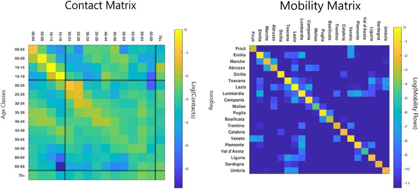
www.nature.com/scientificreports/
Model parameters
β = 0.35 day−1 γ = 1/10 day−1 h = 1/9 day−1
t0 = −30 days ρ = 0.40 α = 0.49
Table 1. Parameters used for the SIOR model.
then, since O(t → ∞) = I(t → ∞) = 0, it follows that R(t → ∞) = N − S(t → ∞) and we recover the same
solution of the SIR model: S(t → ∞) = Ne−R0 [N−S(→∞)].
The Italian lockdown measures of March 8th–9th, 202035,36 aimed to change mobility patterns and to reduce
the intensity of social contacts, both through quarantine measures and by increasing awareness of the importance
of social distancing. We assume the rate γ , which relates to the “medical” evolution of the disease, is not affected
by lockdown, which instead is intended as a non-pharmaceutical intervention to prevent the epidemic spread-
ing. Analogous arguments apply to the rates h and ρ related to the observable compartment (although ρ could
be influenced by different testing schemes or alert thresholds). On the other hand, the transmission coefficient
β can be thought as the product C of a contact rate C times a disease-dependent transmission probability .
Hence, if we assume that the speed of Covid-19 mutation is irrelevant on our timescales, lockdown strategies
mostly influence β by reducing the contact rate C between individuals.
Without loss of generality, we assume that, after the lockdown day tLock = 15 (corresponding to the 9th of
March), the contact rate drops down by a factor α and hence β → αβ. By fitting the observed data Y Obs for a sym-
metric period of 15 days after tLock , and by performing a bootstrap sensitivity analysis, we find α = 0.49 ± 0.01,
i.e. a reduction of ∼ 50% in infectivity and hence in R0. Our analysis is in line with the observed reduction in
R0 in response to combined non-pharmaceutical interventions which has been shown to be on average around
64% compared to the pre-intervention values across several c ountries37.
Table 1 shows the value of the model parameters. Notice that β = 0.35 day−1 corresponds to a basic reproduc-
tion number R0 = 3.5 in line with the average R0 found in Ref.38. Moreover, since patients needing hospitalization
and intensive care represent the highest burden for healthcare facilities, in the figures of the paper we adopt this
value estimated as 3.5% of the total patients, as reported by ISS7, instead of I .
To evaluate the impact of lockdown measures on mobility, we extensively analyze data set on Facebook (FB)
aggregated mobility flows; those data are part of the Facebook project “Data for Good”, and illustrate mobility
patterns of FB users, who allowed the social network to track their location39,40. The data set accounts for daily
movements of approximately 4 M individuals in a period of 1 month, from February 24th to March 24th.
The Facebook mobility data show a reduction in mobility of 15% at Regional level and of 73% at inter-Regional
level during the lockdown phase; however, as we will point out later, mobility has a strong impact at the begin-
ning stage of the epidemic in each single Region/country, while it has much lower effects on its evolution with
each territory.
To characterize the impact of non-pharmaceutical interventions in Italy, we analyze the FB network of mobil-
ity at the province level of detail. The upper panels of Fig. 1 present the evolution of the Italian network of mobility
before and during the national lockdown. This network representation has been obtained by building an averaged
graph over a window of 14 days before and during national lockdown, i.e., each edge has a weight which is the
average of all the observations in such period. While the main mobility hubs such as, Turin, Milan, Bologna,
Rome, and Naples, continue to be connected during the lockdown phase, the Italian peninsula exhibits a mobility
flows network which is severely affected by national lockdown restrictions. As shown by the lower panels of Fig. 1,
the deployment of the lockdown has also reduced both the travelled distance and the flow of travelling people.
Since we are interested in the factors which influence the exit dynamics from lockdown, and not in the accu-
rate quantitative predictions of specific strategies, we rely on scenario analysis, where the lockdown is abruptly
lifted and the system is allowed to return to the pre-lockdown parameters’ configuration. Such an approach clearly
describes a worst-case estimate of the intensity of the second wave of contagion at the end of the lockdown. We
consider several simplified scenarios, where we use the SIOR model described by System (1) with the parameters
presented in Table 1. First, we analyze the relationships between the post-lockdown dynamics and the restrictions
implemented by the national authorities. Second, we modify the framework by introducing a metapopulation
SIOR model to study the effect of explicitly considering Italy as a collection of separate administrative entities
(Regions). Finally, we consider the effects of social interactions across age classes.
Interestingly, mobility flows40 and inter-age social mixing41 display opposite features. In fact, on the one hand,
the social contact matrix is dense (Fig. 2, left panel), indicating that age classes dynamics are strongly coupled.
On the other hand, the inter-Regional mobility matrix is very sparse (Fig. 2, right panel), indicating that Regions
have their own independent dynamics.
National scenarios and exit mechanisms
We first consider a simple exit strategy consisting in lifting the lockdown at a time tUnlock after the peak of O has
occurred. We assume that the infection proceeds uncontrolled up to time tLock when lockdown restrictions are put
in place for the period [tLock , tUnlock ]. During the lockdown phase, we assume that the transmission coefficient β
is reduced by a factor α; finally, we let the parameter β to turn back to its initial value. Hence, such scenario does
not consider other policy interventions, like forcing social distances and the use of personal protection devices
like masks, which may contribute to contain the contagion.
Our results show that lockdown lowers the peak of O—i.e. the individuals with observable symptoms—to
∼ 70% with respect to the free epidemic case, but it also doubles the time of its occurrence from ∼ 1.9 to ∼ 3.8
Scientific Reports | (2020) 10:13764 | https://doi.org/10.1038/s41598-020-70631-9 3
Vol.:(0123456789)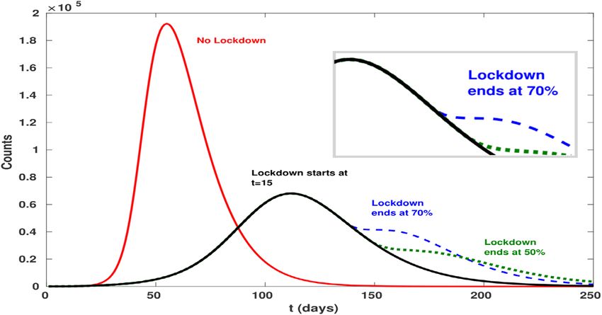
www.nature.com/scientificreports/
Figure 1. Mobility patterns in Italy before and during the lockdown. The upper panels show national mobility
flows (at district level) before and during the lockdown phase. The size of nodes and edges is proportional to
the intra- and inter-district mobility, respectively. The map has been created using Matlab 2019b (see https
://it.mathworks.com/). Lower panels report the distributions of mobility patterns in Italy before and during
the lockdown. The right panel shows the reduction of the travelled distance (in km) and left panel reports the
number of trips before the intervention (blue) and during the lockdown phase (orange).
months, thus constituting an extremely obnoxious effect for the sustainability conditions of the economy of a
country. However, since the number of hospitalized patients and—most importantly—the number of patients
in intensive care is only a fraction of O , lowering the peak puts less stress on the healthcare system. In an ideal
framework, lifting the lockdown when the number of infected people per unit time βS(t)I(t)/N is lower than
the average number of recovering people γ I(t) would ensure that the number of infections would continue to
decrease. In real life, on the other hand, the set-up is more fuzzy: given the lack of information, governments
might decide to resort on some heuristics, such as lifting the lockdown once the observed people O have dropped
to a suitable percentage of the maximum peak. As an example, after ∼ 4.7 months the peak would have reduced
to 70% of its initial value, while after ∼ 5.2 months to 50%. Notice that, the earlier the lockdown is lifted, the
faster O decays to zero even if it starts from higher figures and could possibly induce a second wave of epidemic
spreading. All such effects are shown in Fig. 3 and in Fig. S3 of SI.
Our framework sustains the identification of several mechanisms. The first is related to the timeliness of the
lockdown, i.e. to the choice of anticipating tLock . As expected, anticipating the lockdown (i.e. well before the infec-
tion peak of the uncontrolled epidemic) reduces the height of the peak at the cost of both delaying its appearance
and widening the duration of the epidemic. Conversely, lifting the lockdown too soon can make epidemic to
start again by reaching values higher than the ones observed before the release. A peculiar and counter-intuitive
effect can be generated if the lockdown is anticipated too much: in fact, a too early lockdown may pose the risk
of delaying the start of the epidemic without attenuating its severity.
Scientific Reports | (2020) 10:13764 | https://doi.org/10.1038/s41598-020-70631-9 4
Vol:.(1234567890)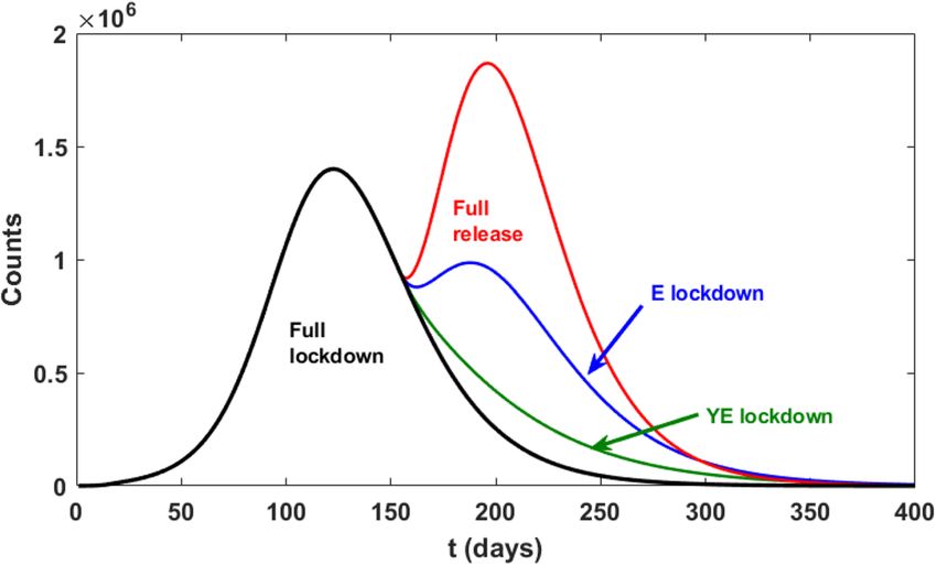
www.nature.com/scientificreports/
Figure 2. Left Panel: social contact matrix (from Ref.41). Right panel: inter-Regional mobility matrix (from
Facebook project39 “Data for Good”). The intensity of the colorbar indicates the strength of a matrix element
(light colors: high values; dark colors: low values). The inter-age social mixing matrix is dense; hence age classes
dynamics are strongly coupled. The inter-Regional mobility flows are very sparse (i.e. off diagonal elements are
order of magnitude lower than diagonal elements). This means that most of the people move within the same
Region of origin; hence, the dynamics of different Regions can be considered as “almost” decoupled.
Figure 3. Comparison of the scenarios where the lockdown is relaxed after the percentage of people with visible
symptoms (O) is reached the 70% and the 50% of the reported cases peak. Lifting the lockdown earlier makes
the epidemic disappear faster, but has higher impact on the number of hospitalized and intensive care patients;
moreover, lifting the lockdown too early can result in a rebound of the number of cases, as shown in the inset.
In addition, increasing the strength α of the lockdown not only delays the time at which it could be lifted,
but it also induces a stronger re-start of the epidemic in the post-lockdown phase. This may trigger the need
for new closures, with repeated lockdown phases that would obviously be unsustainable in terms of social and
economic costs. Specifically, by increasing the strength α of the lockdown, i.e., the ratio between the transmission
β after and before the lockdown, the epidemic peak is pushed forward but its height is lower. On the other hand,
beyond a critical threshold αcrit , the number of Recovered would not grow enough ( R ≪ N ), while I nfected
would quickly decrease to zero; hence, the epidemic would tend to fully recover its strength after the lockdown
lifting, since it would start from a state S ∼ N , R ∼ 0 where the growth of I is again exponential. For instance, in
Fig. S3 in SI, we show the impact of lifting the lockdown when the peak is fallen by 30%, noticing that a stronger
lockdown induces a more consistent upswing of the epidemic. An analogous effect can be observed by varying
Scientific Reports | (2020) 10:13764 | https://doi.org/10.1038/s41598-020-70631-9 5
Vol.:(0123456789)www.nature.com/scientificreports/
the lockdown starting date: anticipating the lockdown ameliorates the epidemic peak by decreasing its height,
but pushes it forward and delays the end of the epidemic.
Contrary to what could be naively expected, an early imposition of the lockdown does not ameliorate the
epidemic: in fact, anticipating too much the lockdown just shifts the timing of the epidemic, leaving its evolution
largely unchanged (see Fig. S4 in SI). This is to be expected every time extreme measures of social distancing are
applied in the very early, exponentially growing, stage of the epidemic. In fact, let us consider two countries A
and B that have the same population, contact matrix, and number of infected people. If A and B decide to estab-
lish a lockdown of strength α at time tA and tB , respectively, then at certain time t any quantity y of the model
would have grown as yA (t) ∼ y 0 eR0 tA eαR0 (t−tA ) and as yB (t) ∼ y 0 eR0 tB eαR0 (t−tB ). If there exists a time t ′ such
that yA (t) = yB (t ′ ), then the epidemic in A and in B will proceed in parallel (even in the non-linear phase) with
a delay t ′ − t . Therefore, if both the epidemic dynamics of A and B are still well approximated by exponential
curves at times t < max{t, t ′ }, then t ′ − t ∝ −(tA − tB ), i.e., the country that has started earlier the lockdown
will experience the same epidemic of the other country, but delayed in time. In particular, for identical initial
conditions, we have that:
1+α
t − t′ = − (tA − tB ) (2)
α
as long as all the times refer to a period before the end of the initial exponential regime. Such an estimate can
be very useful for countries where the epidemic has not yet started. Indeed, calibrating on one own normalized
growth curve the time of the lockdown and its strength would give an idea of how long one can delay the full
start of the epidemic dynamics.
An additional counter-intuitive mechanism can be considered. Since an attenuation of α corresponds to an
effective reproduction number R0eff = αR0, at the critical value αcrit = 1/R0 the epidemic is expected to stay in a
quiescent state where it neither grows nor decreases; to be precise, the decrease becomes sub-exponential, thus
taking a practically infinite time when the size of the population is large. Thus, after tLock the system stays station-
ary until the lockdown is lifted at tUnlock ; at this point, the epidemic starts growing again as it occurred before
the lockdown. In general, if α < αcrit , the epidemic loses strength but as soon as the lockdown is lifted, it starts
again to reach its full strength (see Fig. S5 in SI). Our estimate for the Italian lockdown are α ∼ 0.5 > αcrit ∼ 0.3.
Hence, at least in Regions where epidemic had an early start, it will not be necessary to follow a repeated seek-
and-release strategy in the post-lockdown phase. On the contrary, if it can be attained a lockdown strength
α ∼ αcrit without disrupting the economy, the epidemic could be contained until the creation, production and
distribution of a vaccine.
Regional scenarios
Starting with the first confirmed cases in Lombardy on 21th February, by the beginning of March the Covid-19
outbreak had already spread to the entire Italian territory. While the delay in the beginning of the infection is
accounted for by the different mobility interactions between Italian Regions, once the epidemic has started in
a given area, the intake of external infected people becomes quickly irrelevant. As a consequence, the normal-
ised growth curves of the epidemic variables tend to converge to a similar shape if epidemiological parameters
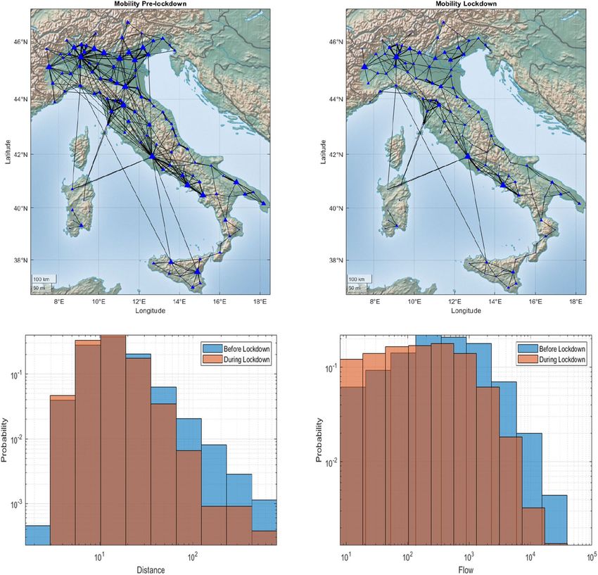
are uniform across the Regions. In fact, according to the Regional info-graphics released by the ISS7, Regional
diffusion curves have a similar behavior but with different starting dates (see Fig. 4A,B). This observation can
be justified as follows: Italian Regions are almost distinct administrative entities, where most of the population
tend to work inside the resident Region42. Hence, the epidemic propagates from Region to Region via the fewer
inter-Regional exchanges (incidentally, Lombardy is the Italian Region which is most involved in international
trade connections43, being a natural candidate for the initial outbreak of the epidemic in Italy).
To test the effects of delayed epidemic starting dates, we build up a synthetic scenario where the Covid-19
outbreak spreads independently in each Region (see “Methods” for the estimation of the experimental time delays
and for the Regional SIOR model); as argued before, given the Italian mobility structure, such an approximation
appears reasonable after the epidemic has started and is even more appropriate during the lockdown phase.
Hence, we apply the parameters of Table 1 to Regional cases, applying System 1 separately to each Region. More
specifically, the maximum number of individuals Ni refers to the population of the ith Region44, while the initial
times of the infection are assumed as those reported in Table 2, where we estimate the time delay by minimiz-
ing the distance among the observed curves. Notice that, assuming Lombardy as the first Region experiencing
the virus contagion (i.e. delay = 0), the resulting Regional delays are mostly correlated to geographical distances
from Lombardy.
By summing up all the Si , . . . , Ri , respectively, we obtain a synthetic model for the global evolution of Covid-
19 epidemic throughout Italy. To evaluate the effect of heterogeneity in time delays, we compare the number of
Delay
daily cases ODelay = Oi in our scenario (obtained
0 by taking into account the Regional delays ti as reported
in Table 2) with the number of daily cases O0 = Oi we would observe by considering the epidemic starting at
the same time t0 in all Regions. As expected, heterogeneity flattens the curve and shifts its maximum later in time.
This is a first source of biases when fitting a heterogeneous dynamics with a global model. Again, we remark here
that we are simply exploring realistic qualitative scenarios, without the aim to predict the real evolution of the
epidemic: in fact, Italian Regions present relevant differences in terms of social contact habits, mobility flows,
organization and capacity of health care provision, as well as for factors that affect the medical parameters, like
comorbidities, social conditions or pollution levels, which should be taken into account to appropriately design
the evolution of the epidemic.
As regards lockdown lifting scenarios, we consider two possible strategies: in the first, that we label the
Delay
Asynchronous scenario, each Region i lifts the lockdown at the time tiUnlock when the peak of Oi decreases
Scientific Reports | (2020) 10:13764 | https://doi.org/10.1038/s41598-020-70631-9 6
Vol:.(1234567890)www.nature.com/scientificreports/
Figure 4. (A,B) analysis of time delays among the start of epidemic in different Regions (see Table 2). If the
dynamics is similar in different Regions, the normalised curves are supposed to be just time shifted versions; (B)
shows that indeed Regional curves have a good collapse when shifted by their delays. (C,D) simulated dynamics
of an Async(hronous) exit strategy (i.e. each Region lifts the lockdown following its own policy) with respect to
a Sync(hronous) exit strategy (i.e. the lockdown lift follows the same policy, but applied to a nation wide scale).
In particular, t Sync corresponds to lifting the lockdown in all the Region after the peak has fallen by 30%, while
Async
ti corresponds to lifting the lockdown in the ith Region after the peak of such Region has fallen by 30%.
Epidemic delays across Italian Regions
Lombardia 0.0 Molise 10.6
Emilia Romagna 3.1 Umbria 11.8
Marche 4.3 Abruzzo 13.1
Veneto 5.7 Lazio 14.5
Valle d’Aosta 6.4 Campania 15.0
P.A. Trento 6.6 Puglia 15.7
P.A. Bolzano 8.0 Sardegna 16.2
Liguria 8.1 Sicilia 16.6
Friuli Venezia Giulia 8.9 Calabria 17.2
Piemonte 9.0 Basilicata 19.2
Toscana 10.4
Table 2. Regional delays (in days). The delay times are calculated by minimising the distance among the
Regional counts of detected infections normalised by the population of the Region. Since Lombardy has been
selected as the reference curve (hence, its delay is 0), the other Regions’ delays are calculated with respect to it.
by 30%; in the second, that we label the Synchronous scenario, each Region i lifts the lockdown at the same time
t Unlock , i.e., when the global peak of ODelay decreases by 30%. The choice of 30% is arbitrary and similar results
would hold for choices of values near the peak (see Fig. S6 in SI); it tries to be a sketch of a situation where, due
to economic pressure, lockdown restrictions are lifted as soon as possible.
The epidemic dynamics in a given Region i is essentially uncorrelated with the epidemic spreading of any
other Region j = i once the outbreak has started. For this reason, it could be appropriate to evaluate the lockdown
lifting time on a Regional basis rather than lifting restrictions at the same time across each Region. Indeed, it
could appear unreasonable to keep locked those Regions where the epidemic started earlier; on the contrary,
Regions where the epidemic began with some delay could experience a strong rebound when subjected to a
premature lockdown lifting. For instance, Fig. 4, panel C and D, shows the effects of lifting the lockdown at both
Regional (Async) and national (Sync) level for two representative Italian Regions, namely Lazio and Lombardy.
Since not only the epidemic, but also economy backslashes are non-linear processes, the Sync scenario can turn
out to be even more disruptive than the epidemic itself (see also Fig. 3 and Table S1 in SI). Notice that analogous
arguments hold—mutatis mutandis—also for the world/countries scenario as long as no super-spreaders45 change
the probability of conveying abroad the epidemic.
Scientific Reports | (2020) 10:13764 | https://doi.org/10.1038/s41598-020-70631-9 7
Vol.:(0123456789)www.nature.com/scientificreports/
Y M E
Y 2.35 0.44 0.67
M 0.47 0.59 0.50
E 0.50 0.55 0.80
Table 3. POLYMOD matrix aggregated for three age classes: Y oung (00−19), M iddle (20−69) and Elderly
(70+). Notice that Y has the highest self-contact rate, followed by E and then by M .
Figure 5. Comparison of the scenarios where the lockdown is relaxed only for a particular age class with
respect to a full release policy. Strategies: YE = quarantine young and elderly, E = quarantine elderly. Notice that
we have purposefully left the M class fully unrestrained in order to show how maintaining a partial, age-based
lockdown could deeply change the effectiveness of the exit strategy, while maintaining active working force
active.
The role of age
As we have already observed in the previous Section, heterogeneity strongly impacts on the estimation of the
results of the model46. Since the transmission coefficient is proportional to the contact rate between individuals,
the rates of social mixing between different age classes represent a well known important source of heteroge-
neity within the model. This information can be estimated either through large-scales surveys41 or through
virtual populations m odeling47. While P OLYMOD41 matrices have been extensively employed to estimate the
cost-effectiveness of vaccination for different age-classes during the 2009 H1N1 pandemic48,49, here we use such
information to support the design of a broad class of exit strategies. Hence, to account for age classes, we extend
our model by rewriting the transmission coefficient as βC (see “Methods” for a full description of the extended
model), where β is the transmission probability of the infection, and C is the matrix describing the contact pat-
terns typical of a given country. Because of lack of further information, we assume β constant among age classes
and C as in Ref.41. To simplify the analysis, we gather POLYMOD age groups into three different classes: Y oung
(00−19), M iddle (20−69) and Elderly (70+) (see Table 3). Such an aggregation combines the most “contactful”
classes (00−19), the classes with the highest mortality risk (70+)7, and—with a good approximation—the classes
corresponding to the active working population (20−69).
Figure 5 shows how the number of people with observed symptoms (O) varies once the age class heterogene-
ity is considered in the model. Differently from Fig. 3, fully lifting the lockdown results in a second wave of the
epidemic, where we observe a higher number of infected cases with respect to the homogeneous case. These
findings highlight the importance of explicitly considering this source of heterogeneity in epidemic models for
preventing underestimations of lockdown lifting consequences.
To estimate the importance of the age classes, we simulate mock-up lockdown release scenarios where some
age classes are kept under lockdown even after the release day. As an example, in an E scenario, the contact rate
of class E among itself and with other classes is damped by a factor α while the contact rates of Y and M among
themselves returns to the pre-lockdown values. Results are shown in Fig. 5 together with the “full release” (i.e.
no dampening of the contact matrix) strategy (see also Table S2 in SI).
Hence, the introduction of the age structure in the model allows us to guide the design of exit strategies based
on age-targeted policies, as a way to dampen a possible upturn of contagion. Specifically, social/physical distance
measures applied to the elderly may contribute to contain the impact of a renewed upward phase, while relaxing
restrictions to the working age class (20–69) would not impair the smoothing of contagion propagation in the
post-lockdown phase. Moreover, different strategies would change the relative percentages of age classes who have
undergone the infection; since the incidence of severe cases is strongly age-related, this is a crucial issue. Again,
Scientific Reports | (2020) 10:13764 | https://doi.org/10.1038/s41598-020-70631-9 8
Vol:.(1234567890)www.nature.com/scientificreports/
it is important to emphasize that we are referring to simple mock-up strategies, which correspond to worst-case
scenarios: in real life, community measures and physical distancing, infection prevention and control, personal
hygiene habits, face mask usage, etc. will be decisive in contributing to dampening the epidemic50.
Conclusions
In this paper we propose and test a general framework to study the Covid-19 contagion through a compartmen-
tal model, with a focus on geographical groups and age classes. Our framework shows that the promptness of
lockdown measures has a main effect on the timing of the contagion. Strict social distancing policies reduce the
severity of the epidemic during the lockdown period, but a full recover of the contagion can occur once such
measures are relaxed. As a consequence, a mix of specific mitigation strategies must be prepared during the
lockdown and implemented thereafter. In order to understand the relative potential impact of different strate-
gies, we focus on two broad decomposition criteria within the model, i.e. on geographical mobility and on social
interactions between age classes. First, we show how local dynamics at Regional level can be erroneously masked
when observing the aggregate national system. Regional heterogeneity tends to lower and widen the curve of the
contagion, contributing to shifting forward in time the epidemic peak at the aggregate level. Second, our analysis
of mobility data shows that, due to the strong sparsity of interconnections across Regions, contagion develops
independently within each Region once the epidemic has started. This, in turn, contributes to account for the
delays observed in the alignment of the contagion curves across different geographical areas. The independ-
ence of Regional dynamics is important, since it could justify the adoption of a mix between general mitigation
strategies and solutions which are specific to individual Regions (or countries) or clusters of Regions. Finally, we
investigate the structure of social contacts across different settings and we quantify the relative importance of
interactions between age classes in the spreading of contagion. We show that the younger (0–19) and the elder
(70+) are the most intensively interacting classes. As a consequence, mitigation strategies specific to behaviours
and interactions of individuals belonging to these two classes can produce a significant impact on diffusion rates
in the post-lockdown phase. Our results show the importance of implementing local preventive and physical
distancing measures specific to the elderly, while providing information, rules and guidelines on behaviours
to be adopted in social interactions, aimed to reduce the risk of contagion for the younger. Overall, our results
provide some guidance on how to lift some of the restrictions on mobility for the active population (20–69),
while smoothing and lessening the propagation of contagion in the post-lockdown phase.
Although our study is tuned on the Italian Covid-19 outbreak, our modeling approach is general enough to
help us understand the role of relevant dimensions, beside the medical and pharmaceutical ones, in identifying
the relative importance of different strategies introduced to contain the epidemic and to mitigate its effects. Our
framework can contribute to mitigate the strength of the trade-off between health and economic outcomes. In
particular, we show how the timeline of post-lockdown measures should take into account some fundamental
compartmental aspects, such as geographical factors and the intensity and frequency of interactions between
members of different age classes in different settings. This feature is general, and it can drive the analysis towards
fine grained simulations on the impact of specific precautionary interventions, which enforce social distancing
acting on proximity/local behaviours while containing the overall burden for the economy and society.
Methods
The proposed SIOR model belongs to the classic family of compartmental models20. As the most renewed SIR
and SEIR (and their variations), it models the infection rate to be proportional to the number of individuals
in a S(usceptible) compartment (i.e., the ones that have never been infected) times the probability of meeting
infected people (modelled as the fraction I/N of I (nfective) individuals respect to the population size N ). The
rate indicating individuals that are Removed from the I class, either because recovered and no more susceptible
or because deceased, is proportional to the number of individuals in I . To have the possibility of calibrating our
model’s parameters with the observed data, we introduce another class O of “observable” individuals, i.e. people
with symptoms strong enough to be detected by the national healthcare system.
Initial parameters estimation. In the early phases of the epidemic, the observed quantities follow an
approximately exponential growth Y Obs ∼ Y0 egt , as expected in most epidemic models. To understand their
implications in our model, we notice that for I/S ≪ 1 we can linearize System 1 resulting in I ∼ I0 e(β−γ )t and
O ∼ ργ I . Thus, minimizing the difference between O and Y Obs in the early period would yield the estimates
for β, γ such that β − γ ∼ g , and R0 ∼ 1 + g/γ would increase linearly with the characteristic time τI = γ −1.
Note that most of the compartmental models based on a set of ordinary differential equations show an initial
exponential growth phase with the same exponent; hence, in the early stage of the epidemic, it is possible to suc-
cessfully fit the “wrong” variables.
To adapt the SIOR’s parameters to the Italian d ata7, we compare the reported cumulative number of Covid-19
cases Y Obs with the analogous quantity Y model = ργ Idt in our model (see Fig. S2 in SI). We want to stress that
our model fitting is not aimed to produce an accurate model for detailed predictions, but to work in a realistic
Region of the parameters space. We estimate model’s parameters by least square fitting on the pre-lockdown
period. Since in such range the data Y Obs show an exponential growth trend, this indicates that the pre-lockdown
period is an early phase of the epidemic where β − γ equals the growth rate of Y Obs. For fixed β − γ , the time
of the epidemic start (that we conventionally assume as the time t0 where the number of infected is 1) and the
fraction ρ of serious cases observed by the national healthcare System, allow some flexibility in estimating the
values of β and γ as long as their difference is fixed. Hence, estimating medical parameters as the rate γ of escap-
ing the infected state is paramount for calibrating the model.
Scientific Reports | (2020) 10:13764 | https://doi.org/10.1038/s41598-020-70631-9 9
Vol.:(0123456789)www.nature.com/scientificreports/
In response to the outbreak of Covid-19, several estimates of model parameters have been proposed in the
literature, revealing a certain amount of uncertainty about some fundamental variables of the epidemic contagion.
The European Centre for Disease controls reports an infection time duration τI between 5 and 14 days50; in our
model, we will use τI = 10 (i.e. γ = τI−1 = 1/10 days−1). According to a report of I SS51, the Italian National
Health Institute, the time from the start of serious symptoms (i.e. when an infected individual results “observed”
from ISS) to the resolution of the symptoms can be estimated as τH ∼ 9 days, corresponding, in our model, to
a value h = 1/9 days−1. Notice that the analysis of 12 different m odels38 reports varying estimates for the basic
reproduction number R0, ranging from 1.5 to 6.47, with mean 3.28 and a median of 2.79.
From fitting the 15 days of Y obs (pre-lockdown phase) and by performing a bootstrap sensitivity analysis
of the parameters, we obtain β − γ ∼ 0.25 ± 0.01 and t0 = −30 ± 5 days by assuming ρ = 40%. Varying ρ in
[10%, 100%] leads β − γ in [0.22, 0.27]. On the other hand, for fixed β − γ , R0 would vary linearly with τI ; as
an example, R0 varies in [2.5, 4.5] for the literature parameters τI ∈ [5, 14]; accordingly, to adjust the difference
in the growth rate, t0 varies in [26, 32]. However, despite the variability of the parameters’ range, the qualitative
behavior of the model—and hence our analysis of the key factors of the epidemic evolution—is unchanged.
Estimation of the experimental regional time delays. We first normalize the observed data by
dividing the number of non-zero observations in a Region for its population. Let yi be the normalized obser-
vations for the ith Region. For each pair of Regions i, j , we define the variation interval ij = [minij , max ij ]
that contains the maximum number of points of both yi and yj , i.e. minij = max{min(yi ), min(yj )} and
max ij = min{max(yi ), max(yj )}. The delay tij between the epidemic start in i and j , respectively, is computed by
minimizing � (�ij ∩ yi (t)) − (�ij ∩ yj (t − tij )�2, where ij ∩ y denotes the values of y falling in the interval ij
and � ·�2 denotes the quadratic norm. Denoting with Ti the times corresponding to the observation in ij ∩ yi , it
is easy to verify that tij = �Ti � − �Tj �, where T
is the average value of the times contained in T .
Equivalence of normalized curves. System 1 referred to Region k becomes:
∂t Sk = −βSk Ik /Nk
∂t Ik = βSk Ik /Nk − γ Ik
∂t Ok = ργ Ik − hOk (3)
∂t Rk = (1 − ρ)γ Ik + hOk
where Nk is the population size of k . By rewriting System (3) in terms of normalized quantities
sk = Sk /Nk , . . . sk = Sk /Nk , we obtain the same set of equations for all the Regions:
∂t s = −βsi
∂t i = βsi − γ i
∂t o = ργ i − ho (4)
∂t r = (1 − ρ)γ i + ho
Hence, for similar initial conditions, by normalizing the experimental observations by the population size, one
should obtain similar epidemic dynamics if the Regional parameters are the same. Notice that, while parameters
like γ are not expected to vary on Regional bases, β is likely to vary since it reflects differences in social interac-
tions. The same reasoning applies to countries or to large, independent administrative units like metropolitan
areas or megacities.
Regional SIOR model. Let us assume of knowing the fraction Zkl of people commuting from Region k to
Region l . Then, System (4) becomes:
∂t sk = −βs k l Zkl il
∂t ik = βsk l Zkl il − γ ik
∂t ok = ργ ik − hok (5)
∂t rk = (1 − ρ)γ ik + hok
From mobility data, we know that ǫk = l�=k Zkl /Zkk ≪ 1 and Zkk ∼ 1; in particular, from Facebook mobil-
ity data we can estimate �ǫk � ∼ 10 . If all the neighbors of a given Region k are fully infected (i.e. il = 1∀l � = k )
−3
and ik (t0 ) = 0, then the variation of ik can be approximated as ∂t ik ∼ ǫk + (β − γ )ik. Namely, as soon as ik > ǫk,
ik will grow exponentially according to ∂t ik ∼ (β − γ )ik and ǫk will become irrelevant, the epidemic dynam-
ics of the Regions will decouple. On the other hand, if epidemic is decaying everywhere, then il ≪ 1∀l � = k ;
thus l =k Zkl il ≪ ǫk and the system again decouple, and the evolution of the epidemic in each Region will be
described by the decoupled equations of System 4.
Social mixing. To take account for social mixing, we rewrite the transmission coefficient as the product of a
transmission probability β times a contact matrix C whose element Cab measure the average number of (physi-
cal) daily contacts among an individual in class age a and an individual in class age b. Notice that the probability
that a susceptible in class a has a contact with an infected in class b is the product of the contact rate Cab times the
probability Ib /Nb that individual in class b is infected. Hence, denoting with Sa , . . . , Ra the number of S(uscepti-
bles),. . .,R(emoved) individuals in class age a, we can rewrite System (1) as:
Scientific Reports | (2020) 10:13764 | https://doi.org/10.1038/s41598-020-70631-9 10
Vol:.(1234567890)www.nature.com/scientificreports/
b
∂t Sa = −βSa b Cab NI b
b
∂t I a = βSa b Cab NI b − γ I a (6)
∂t Oa = ργ I a − hOa
∂t Ra = (1 − ρ)γ I a + hOa
Although the form of System (6) is similar to System (3), here it is not possible to consider a separate evolu-
tion for the different age classes since, differently from the inter-Regional mobility matrix Z , the off diagonal
elements of the social matrix Ca,b , a = b , are of the same order of the diagonal elements Caa , i.e. interactions
among different age classes are of the same magnitude of interactions among individuals of the same age class.
Hence, the exogenous contribute of other classes b = a to the infected growth rate ∂t Ia = b�=a Cab I b /Nb cannot
be disregarded respect the endogenous contribute Caa I a /Na . Obviously, we are not considering the unrealistic
case Na ≫ Nb.
Notice that an equation for the evolution of the total population can be obtained by summing up System (6),
obtaining an equation in S = a Sa , . . . , R = a Ra of the form of System
(1) but with age classes appearing
a I b /N
ab Cab S
in the re-normalized infection parameter β → βC eff , where C eff = SI/N
b
is the average contact value
among infected and susceptible individuals of all age classes. Thus, not taking into account age classes would
lead to measure a time-dependent R0 even with time independent parameters.
Received: 29 April 2020; Accepted: 27 July 2020
References
1. Keeling, M. J. Models of foot-and-mouth disease. Proc. R. Soc. B Biol. Sci. 272(1569), 1195–1202 (2005).
2. Bonaccorsi, G. et al. Economic and social consequences of human mobility restrictions under covid-19. Proc. Natl. Acad. Sci.
117(27), 15530–15535 (2020).
3. Cirillo, P. & Taleb, N. N. Tail risk of contagious diseases. Nat. Phys. 16, 606–613 (2020).
4. Enserink, M., & Kupferschmidt, K. Mathematics of life and death: How disease models shape national shutdowns and other
pandemic policies. Sci. Mag. https://doi.org/10.1126/science.abb8814 (2020).
5. Di Lauro, F., Kiss, I. Z. & Miller, J. The timing of one-shot interventions for epidemic control. medRxiv. https://doi.org/10.1126/
science.abb8814 (2020).
6. Surveillances, V. The epidemiological characteristics of an outbreak of 2019 novel coronavirus diseases (covid-19)-china, 2020.
China CDC Wkly. 2(8), 113–122 (2020).
7. Istituto Superiore di SanitÃ. Iss: Sars-cov-2 dati epidemiologici (https://www.epicentro.iss.it/coronavirus/bollettino/Bollettino
-sorveglianza-integrata-COVID-19_6-aprile-2020.pdf). Technical report, ISS, (2020).
8. Atkeson, A. What will be the economic impact of covid-19 in the us? rough estimates of disease scenarios. Technical report,
National Bureau of Economic Research (2020)
9. Anderson, R. M., Heesterbeek, H., Klinkenberg, D. & Hollingsworth, T. D. How will country-based mitigation measures influence
the course of the covid-19 epidemic?. Lancet 395(10228), 931–934 (2020).
10. McKee, M. & Stuckler, D. If the world fails to protect the economy, covid-19 will damage health not just now but also in the future.
Nat. Med. 26(5), 640–642 (2020).
11. Diekmann, O., Heesterbeek, H. & Britton, T. Mathematical tools for understanding infectious disease dynamics Vol. 7 (Princeton
University Press, Princeton, 2012).
12. Simon, H. A. & Ando, A. Aggregation of variables in dynamic systems. Econometrica: J. Econ. Soc. 29, 111–138 (1961).
13. Ando, A. & Fisher, F. M. Near-decomposability, partition and aggregation, and the relevance of stability discussions. Int. Econ.
Rev. 4(1), 53–67 (1963).
14. Simon, H. A. The Architecture of Complexity (MIT Press, Cambridge, 1996).
15. Courtois, P. J. Decomposability: Queueing and Computer System Applications (Academic Press, London, 2014).
16. Ferguson, N. et al. Report 9: Impact of non-pharmaceutical interventions (npis) to reduce covid19 mortality and healthcare
demand. MRC Centre for Global Infectious Disease Analysis (2020).
17. Prem, K. et al. The effect of control strategies to reduce social mixing on outcomes of the covid-19 epidemic in Wuhan, China: A
modelling study. Lancet Public Health 5, 261–270 (2020).
18. Haushofer, J. & Metcalf, C. J. E. Which interventions work best in a pandemic?. Science 368(6495), 1063–1065 (2020).
19. Chinazzi, M. et al. The effect of travel restrictions on the spread of the 2019 novel coronavirus (covid-19) outbreak. Science
368(6489), 395–400 (2020).
20. Bailey, N.T.J. et al. The mathematical theory of infectious diseases and its applications. Charles Griffin & Company Ltd, 5a Crendon
Street, High Wycombe, Bucks HP13 6LE. (1975).
21. Colizza, V., Barrat, A., Barthelemy, M., Valleron, A. J. & Vespignani, A. Modeling the worldwide spread of pandemic influenza:
baseline case and containment interventions. PLoS Med. 4(1), e13 (2007).
22. Colizza, V. & Vespignani, A. Epidemic modeling in metapopulation systems with heterogeneous coupling pattern: Theory and
simulations. J. Theor. Biol. 251(3), 450–467 (2008).
23. Balcan, D. et al. Multiscale mobility networks and the spatial spreading of infectious diseases. Proc. Natl. Acad. Sci. USA. 106(51),
21484–21489 (2009).
24. Keeling, M. J. & Rohani, P. Modeling infectious diseases in humans and animals (Princeton University Press, Princeton, 2011).
25. Aleta, A. et al. Modeling the impact of social distancing, testing, contact tracing and household quarantine on second-wave sce-
narios of the covid-19 epidemic (2020).
26. Banerjee, A. et al. Estimating excess 1-year mortality associated with the covid-19 pandemic according to underlying conditions
and age: a population-based cohort study. Lancet Public Health 395, 1715–1725 (2020).
27. Eikenberry, S. E. et al. To mask or not to mask: Modeling the potential for face mask use by the general public to curtail the covid-
19 pandemic. Infect. Dis. Model 5, 293–308 (2020).
28. Hou, C. et al. The effectiveness of quarantine of Wuhan city against the corona virus disease 2019 (covid-19): A well-mixed seir
model analysis. J. Med. Virol. 92, 841–848 (2020).
29. Jia, J. S., Lu, X., Yuan, Y. et al. Population flow drives spatio-temporal distribution of covid-19 in China. Nature 582, 389–394
(2020).
Scientific Reports | (2020) 10:13764 | https://doi.org/10.1038/s41598-020-70631-9 11
Vol.:(0123456789)www.nature.com/scientificreports/
30. Van Bavel, J.J. et al. Using social and behavioural science to support covid-19 pandemic response. Nat. Hum. Behav. 1–12 (2020).
31. Casella, F. Can the covid-19 epidemic be managed on the basis of daily data? arXiv preprint arXiv :2003.06967 (2020).
32. Funk, S., Salathé, M. & Jansen, V. A. Modelling the influence of human behaviour on the spread of infectious diseases: a review. J.
R. Soc. Interface 7(50), 1247–1256 (2010).
33. Bai, Y. et al. Presumed asymptomatic carrier transmission of COVID-19. JAMA 323(14), 1406–1407 (2020).
34. Nishiura, H. et al. Estimation of the asymptomatic ratio of novel coronavirus infections (covid-19). medRxiv 94, 154 (2020).
35. Presidenza del Consiglio dei Ministri. Ulteriori disposizioni attuative del decreto-legge 23 febbraio 2020, n. 6, recante misure
urgenti in materia di contenimento e gestione dell’emergenza epidemiologica da covid-19. Gazzetta Ufficiale, Decreto del Presidente
del Consiglio dei Ministri, 59 (08-03-2020) (2020).
36. Presidenza del Consiglio dei Ministri. Ulteriori disposizioni attuative del decreto-legge 23 febbraio 2020, n. 6, recante misure
urgenti in materia di contenimento e gestione dell’emergenza epidemiologica da covid-19. Gazzetta Ufficiale, Decreto del Presidente
del Consiglio dei Ministri, 62 (09-03-2020) (2020).
37. Flaxman, S. et al. Report 13: Estimating the number of infections and the impact of non-pharmaceutical interventions on covid-19
in 11 European countries (2020).
38. Liu, Y., Gayle, A.A., Wilder-Smith, A. & Rocklöv, J. The reproductive number of covid-19 is higher compared to sars coronavirus.
J. Travel Med. (2020).
39. Facebook. Data for good facebook (https://dataforgood.fb.com/docs/Covid-19/). Technical report.
40. Buckee, C. O. et al. Aggregated mobility data could help fight COVID-19. Science 368(6487), 145 (2020).
41. Mossong, J. et al. Social contacts and mixing patterns relevant to the spread of infectious diseases. PLoS Med. 5(3), e74 (2008).
42. Istituto Nazionale di Statistica. Popolazione insistente per studio e lavoro (https://www.istat.it/it/files//2020/03/Popolazione-insis
tente.pdf). Technical report, ISTAT (2020).
43. Istituto Nazionale di Statistica. Commercio estero (https://www.istat.it/it/commercio-estero). Technical report, ISTAT (2020).
44. Istituto Nazionale di Statistica. Census data italian pupulation (https://www.istat.it/it/popolazione-e-famiglie?dati). Technical
report, ISTAT (2020).
45. Pastor-Satorras, R. & Vespignani, A. Epidemic spreading in scale-free networks. Phys. Rev. Lett. 86(14), 3200 (2001).
46. Diekmann, O., Heesterbeek, J. A. & Metz, J. A. On the definition and the computation of the basic reproduction ratio r 0 in models
for infectious diseases in heterogeneous populations. J. Math. Biol. 28(4), 365–382 (1990).
47. Fumanelli, L., Ajelli, M., Manfredi, P., Vespignani, A. & Merler, S. Inferring the structure of social contacts from demographic data
in the analysis of infectious diseases spread. PLoS Comput. Biol. 8(9), e1002673 (2012).
48. Medlock, J. & Galvani, A. P. Optimizing influenza vaccine distribution. Science 325(5948), 1705–1708 (2009).
49. Baguelin, M. et al. Vaccination against pandemic influenza a/h1n1v in England: A real-time economic evaluation. Vaccine 28(12),
2370–2384 (2010).
50. European Centre for Disease Prevention and Control (ECDC). Coronavirus disease 2019 (covid-19) pandemic: increased trans-
mission in the eu/eea and the UK—eigth update, 8 April 2020 (2020).
51. COVID-19 Surveillance Group, and Istituto Superiore di Sanità (ISS). Characteristics of covid-19 patients dying in Italy report
based on available data on March 30th, 2020 (2020).
Acknowledgements
A.S., E.B., M.C. and W.Q. acknowledge the support from CNR P0000326 project AMOFI (Analysis and Models
OF social medIa) and CNR-PNR National Project DFM.AD004.027 “ Crisis-Lab”.
Author contributions
All authors contributed to the writing an the discussion of the paper. A.Sc. contributed to the modelling and the
simulations. M.C., E.B., A.F and A.Sp. contributed to the data retrieval and analysis. A.Sc. and E.B. contributed
to the mathematical analysis of the models. A.Sc., F.P. and W.Q. contributed to the design of the paper and of
the strategies to be analysed. F.P., A.F. and A.Sp. contributed to the discussion of the economic impacts of the
analysis. W.Q. and M.C. contributed to the mobility analysis.
Competing interests
The authors declare no competing interests.
Additional information
Supplementary information is available for this paper at https://doi.org/10.1038/s41598-020-70631-9.
Correspondence and requests for materials should be addressed to A.S.
Reprints and permissions information is available at www.nature.com/reprints.
Publisher’s note Springer Nature remains neutral with regard to jurisdictional claims in published maps and
institutional affiliations.
Open Access This article is licensed under a Creative Commons Attribution 4.0 International
License, which permits use, sharing, adaptation, distribution and reproduction in any medium or
format, as long as you give appropriate credit to the original author(s) and the source, provide a link to the
Creative Commons license, and indicate if changes were made. The images or other third party material in this
article are included in the article’s Creative Commons license, unless indicated otherwise in a credit line to the
material. If material is not included in the article’s Creative Commons license and your intended use is not
permitted by statutory regulation or exceeds the permitted use, you will need to obtain permission directly from
the copyright holder. To view a copy of this license, visit http://creativecommons.org/licenses/by/4.0/.
© The Author(s) 2020
Scientific Reports | (2020) 10:13764 | https://doi.org/10.1038/s41598-020-70631-9 12
Vol:.(1234567890)You can also read