Unsupervised User Stance Detection on Twitter - Association ...
←
→
Page content transcription
If your browser does not render page correctly, please read the page content below
Proceedings of the Fourteenth International AAAI Conference on Web and Social Media (ICWSM 2020)

                              Unsupervised User Stance Detection on Twitter
                     Kareem Darwish,1 Peter Stefanov,2 Michaël Aupetit,1 Preslav Nakov1
                                               1
                                                 Qatar Computing Research Institute
                                           Hamad bin Khalifa University, Doha, Qatar
                                            2
                                              Faculty of Mathematics and Informatics,
                                     Sofia University ”St. Kliment Ohridski”, Sofia, Bulgaria
                               {kdarwish, maupetit, pnakov}@hbku.edu.qa, p.stefanov@hotmail.com

                            Abstract                                        In either case, some form of initial manual labeling of tens
                                                                            or hundreds of users is performed, followed by user-level su-
  We present a highly effective unsupervised framework for de-              pervised classification or label propagation based on the user
  tecting the stance of prolific Twitter users with respect to con-          accounts and the tweets that they retweet and/or the hashtags
  troversial topics. In particular, we use dimensionality reduc-            that they use (Magdy et al. 2016; Pennacchiotti and Popescu
  tion to project users onto a low-dimensional space, followed
  by clustering, which allows us to find core users that are rep-
                                                                            2011a; Wong et al. 2013).
  resentative of the different stances. Our framework has three                Retweets and hashtags can enable such classification as
  major advantages over pre-existing methods, which are based               they capture homophily and social influence (DellaPosta,
  on supervised or semi-supervised classification. First, we do              Shi, and Macy 2015; Magdy et al. 2016), both of which
  not require any prior labeling of users: instead, we create               are phenomena that are readily apparent in social media.
  clusters, which are much easier to label manually afterwards,             With homophily, similarly minded users are inclined to cre-
  e.g., in a matter of seconds or minutes instead of hours. Sec-            ate social networks, and members of such networks exert so-
  ond, there is no need for domain- or topic-level knowledge
                                                                            cial influence on one another, leading to more homogeneity
  either to specify the relevant stances (labels) or to conduct the
  actual labeling. Third, our framework is robust in the face of            within the groups. Thus, members of homophilous groups
  data skewness, e.g., when some users or some stances have                 tend to share similar stances on various topics (Garimella
  greater representation in the data. We experiment with dif-               2017). Moreover, the stances of users are generally stable,
  ferent combinations of user similarity features, dataset sizes,           particularly over short time spans, e.g., over days or weeks.
  dimensionality reduction methods, and clustering algorithms               All this facilitates both supervised classification and semi-
  to ascertain the most effective and most computationally ef-              supervised approaches such as label propagation. Yet, exist-
  ficient combinations across three different datasets (in En-               ing methods are characterized by several drawbacks, which
  glish and Turkish). We further verified our results on addi-               require an initial set of labeled examples, namely: (i) man-
  tional tweet sets covering six different controversial topics.            ual labeling of users requires topic expertise in order to prop-
  Our best combination in terms of effectiveness and efficiency
                                                                            erly identify the underlying stances; (ii) manual labeling also
  uses retweeted accounts as features, UMAP for dimension-
  ality reduction, and Mean Shift for clustering, and yields a              takes substantial amount of time, e.g., 1–2 hours or more for
  small number of high-quality user clusters, typically just 2–             50–100 users; and (iii) the distribution of stances in a sam-
  3, with more than 98% purity. The resulting user clusters can             ple of users to be labeled, e.g., the n most active users or
  be used to train downstream classifiers. Moreover, our frame-              random users, might be skewed, which could adversely af-
  work is robust to variations in the hyper-parameter values and            fect the classification performance, and fixing this might re-
  also with respect to random initialization.                               quire non-trivial hyper-parameter tweaking or manual data
                                                                            balancing.
                                                                               Here we aim at performing stance detection in a com-
                        Introduction                                        pletely unsupervised manner to tag the most active users on
Stance detection is the task of identifying the position of a               a topic, which often express strong views. Thus, we over-
user with respect to a topic, an entity, or a claim (Mohammad               come the aforementioned shortcomings of supervised and
et al. 2016), and it has broad applications in studying public              semi-supervised methods. Specifically, we automatically de-
opinion, political campaigning, and marketing. Stance de-                   tect homogeneous clusters, each containing a few hundred
tection is particularly interesting in the realm of social me-              users or more, and then we let human analysts label each
dia, which offers the opportunity to identify the stance of                 of these clusters based on the common characteristics of the
very large numbers of users, potentially millions, on differ-               users therein such as the most representative retweeted ac-
ent issues. Most recent work on stance detection has focused                counts or hashtags. This labeling of clusters is much cheaper
on supervised or semi-supervised classification.                             than labeling individual users. The resulting user groups can
                                                                            be used directly, and they can also serve to train supervised
Copyright  c 2020, Association for the Advancement of Artificial            classifiers or as seeds for semi-supervised methods such as
Intelligence (www.aaai.org). All rights reserved.                           label propagation.

                                                                      141
Overall, we experiment with different sampled subsets from
three different tweet datasets with gold stance labels in dif-
ferent languages and covering various topics, and we show
that we can identify a small number of user clusters (2-3
clusters) composed of hundreds of users on average with
purity in excess of 98%. We further verify our results on
additional tweet datasets covering six different controversial
topics.
Our contributions can be summarized as follows:
• We introduce a robust stance detection framework for au-
tomatically discovering core groups of users without the
need for manual intervention, which enables subsequent
manual bulk labelling of all users in a cluster at once.
• We overcome key shortcomings of existing supervised
and semi-supervised classification methods such as the
Figure 1: Overview of our stance detection pipeline, the op- need for topic-informed manual labeling and for handling
tions studied in this paper, and the benefits they offer. In bold class imbalance and the presence of potential skews.
font: best option in terms of accuracy. In bold red: the best • We show that dimensionality reduction techniques such
option both in terms of accuracy and computing time. as FD and UMAP, followed by Mean Shift clustering, can
effectively identify core groups of users with purity in ex-
cess of 98%.
Our method works as follows (see also Figure 1): given a set
of tweets on a particular topic, we project the most active • We demonstrate the robustness of our method to
users onto a two-dimensional space based on their similar- changes in dimensionality reduction and clustering hyper-
ity, and then we use peak detection/clustering to find core parameters as well as changes in tweet set size, kinds of
groups of similar users. Using dimensionality reduction has features used to compute similarity, and minimum num-
several desirable effects. First, in a lower dimensional space, ber of users, among others. In doing so, we ascertain the
good projection methods bring similar users closer together minimum requirements for effective stance detection.
while pushing dissimilar users further apart. User visualiza- • We elucidate the computational efficiency of different
tion in two dimensions also allows an observer to ascertain combinations of features, user sample size, dimensional-
how separable users with different stances are. ity reduction, and clustering.
Dimensionality reduction further facilitates downstream
clustering, which is typically less effective and less efficient Background
in high-dimensional spaces. Using our method, there is no
need to manually specify the different stances a priori. In- Stance Classification: There has been a lot of recent
stead, these are discovered as part of clustering, and can be research interest in stance detection with focus on infer-
easily labeled in a matter of minutes at the cluster level, ring a person’s or an article’s position with respect to a
e.g., based on the most salient retweets or hashtags for a topic/issue or political preferences in general (Barberá 2015;
cluster. Moreover, our framework overcomes the problem of Barberá and Rivero 2015; Borge-Holthoefer et al. 2015;
class imbalance and the need for expertise about the topic. Cohen and Ruths 2013; Colleoni, Rozza, and Arvidsson
2014; Conover et al. 2011b; Fowler et al. 2011; Himel-
In our experiments, we compare different variants of our
boim, McCreery, and Smith 2013; Magdy et al. 2016;
stance detection framework. In particular, we experiment
Magdy, Darwish, and Weber 2016; Makazhanov, Rafiei, and
with three different dimensionality reduction techniques,
Waqar 2014; Mohtarami et al. 2018; Mohtarami, Glass, and
namely the Fruchterman-Reingold force-directed (FD)
Nakov 2019; Stefanov et al. 2020; Weber, Garimella, and
graph drawing algorithm (Fruchterman and Reingold 1991),
Batayneh 2013).
t-Distributed Stochastic Neighbor Embeddings (t-SNE)
(Maaten and Hinton 2008), and Uniform Manifold Approx-
imation and Projection (UMAP) algorithm (McInnes and Effective Features: Several studies have looked at fea-
Healy 2018). For clustering, we compare DBSCAN (Ester et tures that may help reveal the stance of users. This in-
al. 1996) and Mean Shift (Comaniciu and Meer 2002), both cludes textual features such as the text of the tweets and
of which can capture arbitrarily shaped clusters. We also ex- hashtags, network interactions such as retweeted accounts
periment with different features such as retweeted users and and mentions as well as follow relationships, and pro-
hashtags as the basis for computing the similarity between file information such as user description, name, and lo-
users. The successful combinations use FD or UMAP for di- cation (Borge-Holthoefer et al. 2015; Magdy et al. 2016;
mensionality reduction, Mean Shift for peak detection, and Magdy, Darwish, and Weber 2016; Weber, Garimella, and
retweeted accounts to compute user similarity. We also ex- Batayneh 2013). Using network interaction features, specif-
plore robustness with respect to hyper-parameters and the ically retweeted accounts, was shown to yield better results
required minimum number of tweets and users. compared to using content features (Magdy et al. 2016).
142User Classification: Most studies focused on supervised tially with the increase in dimensionality as there are many
or semi-supervised methods, which require an initial seed more possible patterns than in lower-dimensional subspaces;
set of labeled users. Label propagation was used to au- and the computation time and the memory needed for clus-
tomatically tag users based on the accounts they follow tering also grow. Moreover, it has been shown that as dimen-
(Barberá 2015) and retweets (Borge-Holthoefer et al. 2015; sionality increases, the distance from any point to the near-
Weber, Garimella, and Batayneh 2013). Although it has very est data point approaches the distance to the furthest data
high precision (often above 95%), it has three drawbacks: point (Beyer et al. 1999). This is problematic for clustering
(i) it tends to label users who are more extreme in their techniques, which typically assume short within-cluster and
views, (ii) careful manipulation of thresholds may be re- large between-cluster distances. We conducted experiments
quired, particularly when the initial tagged user set is imbal- that involved clustering directly in the high-dimensional fea-
anced, and (iii) post checks are needed. Some of these issues ture space and all of them failed to produce meaningful clus-
can be observed in the Datasets section below, where two of ters. On the other hand, most clustering techniques are very
our test sets were constructed using label propagation. Our efficient in low-dimensional spaces.
method overcomes the latter two drawbacks. Another issue comes from the need for human experts to
Supervised classification was used to assign stance la- ascertain the validity of the clustering result beyond stan-
bels, where classifiers were trained using a variety of fea- dard clustering statistics. For instance, an expert may want
tures such as tweet text, hashtags, user profile informa- to verify that users belong to the core of separable groups
tion, retweeted accounts or mentioned accounts (Magdy such that they are good representatives of the groups and
et al. 2016; Magdy, Darwish, and Weber 2016; Pennac- good candidate seeds for possible subsequent classification.
chiotti and Popescu 2011a). Such classification can label Visualization has come as a natural way to support the
users with precision typically ranging between 70% and experts using Dimensionality Reduction (DR) or Multi-
90%. Rao et al. (2010) used socio-linguistic features that Dimensional Projection (MDP) (Nonato and Aupetit 2018).
include types of utterances, e.g., emoticons and abbrevia- Different pipelines combining Dimensionality Reduction
tions, and word n-grams to distinguish between Republi- and Clustering have been studied (Wenskovitch et al. 2018)
cans and Democrats with more than 80% accuracy. Pennac- in Visual Analytics in order to support user decision, giving
chiotti and Popescu (2011a) extended the work of Rao et guidelines to select the best approach for a given applica-
al. (2010) by introducing features based on profile infor- tion. As our primary goal is to support users to check cluster
mation (screen name, profile description, followers, etc.), quality visually and label data based on cluster information,
tweeting behavior, socio-linguistic features, network inter- and given that clustering is more efficient in low dimension-
actions, and sentiment. It has been shown that users tend to ality, we decided to first reduce data dimensionality and then
form so-called “echo chambers”, where they engage with to apply clustering in the projection space.
like-minded users (Himelboim, McCreery, and Smith 2013; Among the MDP techniques, the Force Directed (FD)
Magdy et al. 2016), and they also show persistent beliefs graph drawing technique (Fruchterman and Reingold 1991),
over time and tend to maintain their echo chambers, which the t-distributed Stochastic Neighbor Embedding (t-SNE),
reveal significant social influence (Borge-Holthoefer et al. (Maaten and Hinton 2008) and the recent Uniform Man-
2015; Magdy et al. 2016; Pennacchiotti and Popescu 2011b). ifold Approximation and Projection technique (UMAP),
Duan et al. (2012) used the so-called “collective classifi- (McInnes and Healy 2018), have been widely used for di-
cation” techniques to jointly label the interconnected net- mensionality reduction. They transform high-dimensional
work of users using both their attributes and their relation- data into two-dimensional scatter plot representations while
ships. Since there are implicit links between users on Twit- preserving data similarity, and hence possible clusters.
ter (e.g., they retweet the same accounts or use the same Regarding the clustering techniques that could be used in
hashtags), collective classification is relevant here. Darwish the resulting 2D space, we can select them based on their
et al. (2017) extended this idea by employing a so-called lower computational complexity, their ability to find groups
user similarity space of lower dimensionality to improve su- with various shapes, and the number of hyper-parameters to
pervised stance classification. There was a related SemEval- tune. Moreover, we are interested in detecting the core clus-
2016 (Mohammad et al. 2016) task on stance detection, but ters that are likely to generate strong stances, rather than
it was at the tweet level, not user level. noisy sparse clusters with low influence. DBSCAN (Ester
et al. 1996) and Mean Shift (Comaniciu and Meer 2002)
are two well-known clustering techniques that satisfy these
Dimensionality Reduction and Clustering: A poten- constraints and further enable the discovery of core clus-
tial unsupervised method for stance detection may involve ters and high-density peaks, respectively, with low compu-
user clustering. Beyond the selection of relevant features tational complexity and fewer hyper-parameters to tune.
for stance detection, a major challenge for clustering ap- In this work, we explore combinations of (i) relevant in-
proaches is the number of features. Indeed, an expert may put features, namely retweeted tweets, retweeted accounts,
be willing to use as many meaningful input features as pos- and hashtags, (ii) dimensionality reduction of these input
sible, expecting the machine to detect automatically the rel- spaces into two dimensions using FD, t-SNE and UMAP,
evant ones for the task at hand. This high-dimensional space and (iii) clustering thereafter using DBSCAN and Mean
is subject to the curse of dimensionality (Verleysen and oth- Shift, to determine the most efficient pipeline for finding
ers 2003): the search space for a solution grows exponen- stance clusters (see Figure 1).
143Finding Stance Clusters • UMAP (McInnes and Healy 2018) is similar to t-SNE,
Feature Selection: Given a tweet dataset that has been but assumes that the data points are uniformly distributed
pre-filtered using topical words, we take the n most “en- on a Riemannian connected manifold with a locally con-
gaged” users who have posted a minimum number of tweets stant metric. A fuzzy topological structure encoded as a
in the dataset. Given this sample of users, we compute the weighted K-Nearest Neighbor graph of the data points is
cosine similarity between each pair of users. This similar- used to model that manifold and its uniform metric. The
ity can be computed based on a variety of features includ- same structure is built in the projection space across the
ing (re)tweeting identical tweets, which is what is typically points representing the data, and their position is updated
used in label propagation; the hashtags that users use; or to minimize the divergence between these two structures
the accounts they retweet. Thus, the dimensions of the fea- (McInnes and Healy 2018). UMAP is significantly more
ture spaces given the different features are the number of computationally efficient than t-SNE and tends to empha-
unique tweets (feature space T), the number of unique hash- size the cluster structure in the projection. We used Leland
tags (feature space H), or the number of unique retweeted McInnes’s implementation of UMAP.3
accounts (feature space R).
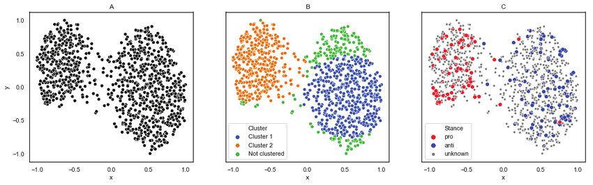
We computed the cosine similarity using each of these Clustering: After projecting the users into a two-
feature spaces independently as well as concatenating all of dimensional space, we scale user positions in x and y (in-
them together (below, we will refer to this combination as dependently) between −1 and 1 (as shown in the successful
TRH). For example, when constructing a user’s sparse fea- plot A in Figure 2 and in the less successful plot in Figure 3)
ture vector using retweeted accounts (Feature space R), the and we proceed to identify cluster cores using the following
elements in the vector would be all 0 except for the retweeted two clustering methods (see plot B in Figure 2):
accounts, where it would correspond to their relative fre-
quency, i.e., the number of times the user has retweeted each • DBSCAN is a density-based clustering technique which
of them in our dataset divided by the number of times the attempts to identify clusters based on preset density (Es-
user has retweeted any of them. For instance, if the user has ter et al. 1996). It can identify clusters of any shape, but it
retweeted three accounts with frequencies 5, 100, and 895, requires tuning two hyper-parameters related to clustering
then the corresponding feature values would be 5/1,000, density: , which specifies how close the nodes have to be
100/1,000, and 895/1,000, where 1,000 is the sum of the fre- in order to be considered “reachable” neighbors, and m,
quencies. which is the minimum number of nodes required to form
a core set. Points that are not in a core set nor reachable
by any other points are outliers that are not considered as
Dimensionality Reduction: We experimented with the part of the final clusters. We used the scikit-learn imple-
following dimensionality reduction techniques based on the mentation of DBSCAN.
aforementioned cosine similarity between users: • Mean Shift attempts to find peaks of highest density
• FD (Fruchterman and Reingold 1991) minimizes the based on a kernel smoothing function (Comaniciu and
energy in the representation of the network as a low- Meer 2002), typically using a Gaussian kernel. With a
dimensional node-link diagram, analogous to a physical kernel at each point, each point is iteratively shifted to
system, where edges are springs and nodes bear repulsive the mean (barycenter) of all the points weighted by its
charges such that similar nodes are pulled closer together kernel. All points thus converge to the local maximum of
and dissimilar nodes are pushed further apart. In our ex- the density nearby them. The kernel’s bandwidth hyper-
periments, we used the implementation in the NetworkX parameter determines the number of peaks detected by
toolkit.1 Mean Shift and all points converging to the same peak
are grouped into the same cluster. The bandwidth can be
• t-SNE (Maaten and Hinton 2008) uses the pre-computed estimated automatically using cross-validation in a prob-
cosine similarity between pairs of users in order to es- abilistic setting. Orphan peaks where only a few points
timate the probability for a user to be the neighbor of converge are assumed to be outliers and hence are not
another one in the high-dimensional space — the farther clustered. Again, we used the scikit-learn implementation
apart they are in terms of cosine similarity, the lower the of the algorithm.
probability that they are neighbors. A set of points repre-
senting the users is located in the low-dimensional space
and the same probabilistic matrix is computed based on Labeling Clusters: Finally, we assume that the users in
the relative Euclidean distances in that projection space. each cluster would have the same stance with respect to the
The position of the points is updated progressively try- target topic. As we will show later, we are able to find the
ing to minimize the Kullback-Leibler divergence between most salient retweeted accounts and hashtags for each user
these two probability distributions (Maaten and Hinton cluster using a variant of the valence score (Conover et al.
2008). In our experiments, we used the scikit-learn2 im- 2011a). This score can help when assigning labels to user
plementation of t-SNE. clusters, based on the most frequent characteristics of the
group.
1
http://networkx.github.io/
2 3
https://scikit-learn.org http://umap-learn.readthedocs.io/en/latest/
144Figure 2: Successful setup: Plot (A) illustrates how user vectors get embedded by UMAP in two dimensions, Plot (B) presents
the clusters Mean Shift produces for them, and Plot (C) shows the users’ true labels.
Cruz, Sasse, Flake, Crapo, Tillis, Kennedy, Feinstein, Leahy,
Durbin, Whitehouse, Klobuchar, Coons, Blumenthal, Hi-
rono, Booker, and Harris. These keywords include the
judge’s name, his main accuser, and the names of the mem-
bers of the Senate’s Judiciary Committee. In the process,
we collected 23 million tweets, authored by 687,194 users.
Initially, we manually labeled the 50 users who posted the
highest number of tweets in our dataset. It turned out that
35 of them supported the Kavanaugh’s nomination (labeled
as pro) and 15 opposed it (labeled as anti). Next, we used
label propagation to automatically label users based on their
retweet behavior (Darwish et al. 2017; Kutlu, Darwish, and
Elsayed 2018; Magdy et al. 2016). The assumption here is
that users who retweet a tweet on the target topic are likely
Figure 3: Unsuccessful setup: The user vectors after projec- to share the same stance as the one expressed in that tweet.
tion (using t-SNE in this case); the colors show the users’ Given that many of the tweets in our collection were actu-
true labels. ally retweets or duplicates, we labeled users who retweeted
15 or more tweets that were authored or retweeted by the
pro group with no retweets from the other group as pro.
Datasets Similarly, we labeled users who retweeted 6 or more tweets
We used two types of datasets: labeled and unlabeled. We from the anti group and no retweets from the other side as
pre-labeled the former in advance, and then we used it to anti.
try different experimental setups and hyper-parameters val-
ues. Additionally, we collected fresh unlabeled data on new We chose to increase the minimum number for the pro
topics and we applied the best hyper-parameters on this new group as they were over-represented in the initial manually
data. labeled set. We performed only one label propagation iter-
ation, labeling 48,854 users: 20,098 as pro and 28,756 as
Labeled Datasets anti. Since we do not have gold labels to compare against,
we opted to spot-check the results. Thus, we randomly se-
We used three datasets in different languages: lected 50 automatically labeled accounts (21 pro and 29
1. Kavanaugh dataset (English): We collected tweets per- anti), and we manually labeled them. All automatic labels
taining to the nomination of Judge Kavanaugh to the US matched the manual labels. As observed, label propagation
Supreme Court in two different time intervals, namely may require some tuning to work properly, and checks are
September 28-30, 2018, which were the three days fol- needed to ensure efficacy.
lowing the congressional hearing concerning the sexual as-
sault allegation against Kavanaugh, and October 6-9, 2018, 2. Trump dataset (English): We collected 4,152,381
which included the day the Senate voted to confirm Ka- tweets (from 1,129,459 users) about Trump and the 2018
vanaugh and the following three days. We collected tweets midterm elections from Twitter over a period of three
using the Twarc toolkit,4 where we used both the search days (Oct. 25-27, 2018) using the following keywords:
and the filtering interfaces to find tweets containing any Trump, Republican, Republicans, Democrat, Democrats,
of the following keywords: Kavanaugh, Ford, Supreme, ju- Democratic, midterm, elections, POTUS (President of the
diciary, Blasey, Grassley, Hatch, Graham, Cornyn, Lee, US), SCOTUS (Supreme Court of the US), and candi-
date. We automatically labeled 13,731 users based on
4
https://github.com/edsu/twarc the hashtags that they used in their account descrip-
145tions. Specifically, we labeled 7,421 users who used Topic Keywords Date No. of
Range Tweets
the hashtag #MAGA (Make American Great Again) as
pro Trump and 6,310 users who used any of the Gun con- #gun, #guns, #weapon, #2a, Feb 1,782,384
trol/rights #gunviolence, #secondamend- 25–Mar
hashtags #resist, #resistance, #impeachTrump, ment, #shooting, #massshoot- 3, 2019
#theResistance, or #neverTrump as anti. We fur- ing, #gunrights, #GunReform-
ther tried label propagation, but it increased the number of Now, #GunControl, #NRA
labeled users by 12% only; thus, we dropped it. In order to Ilhan Omar IlhanOmarIsATrojanHorse, Mar 1– 2,556,871
remarks on #IStandWithIlhan, #ilhan, #An- 9, 2019
check the quality of the automatic labeling, we randomly Israel lobby tisemitism, #IlhanOmar, #Il-
labeled 50 users, and we found out that for 49 of them, the hanMN, #RemoveIlhanOmar,
manual labels matched the automatic ones. #ByeIlhan, #RashidaTlaib,
#AIPAC, #EverydayIslamopho-
bia, #Islamophobia, #ilhan
3. Erdoğan dataset (Turkish): We collected a total of Illegal #border, #immigration, #immi- Feb 2,341,316
19,856,692 tweets (authored by 3,184,659 users) about immigration grant, #borderwall, #migrant, 25–Mar
Erdoğan and the June 24, 2018 Turkish elections that cover #migrants, #illegal, #aliens 4, 2019
Midterm midterm, election, elections Oct 520,614
the period of June 16–23, 2018 (inclusive). Unlike the pre- 25–27,
vious two datasets, which were both in English, this one 2018
was in Turkish. We used many election-related terms in- Racism #blacklivesmatter, #bluelives- Feb 2,564,784
cluding political party names, names of popular politicians, & police matter, #KKK, #racism, #racist, 25–Mar
and election-related hashtags. We were interested in users’ brutality #policebrutality, #excessive- 3, 2019
force, #StandYourGround,
stance toward Erdoğan, the incumbent presidential candi- #ThinBlueLine
date, specifically. In order to label users with their stance, Vaccination #antivax, #vaxxing, #Big- Mar 1– 301,209
we made one simplifying assumption, namely that the sup- benefits & Pharma, #antivaxxers, #measle- 9, 2019
porter of a particular political party would be supporting dangers soutbreak, #Antivacine,
#VaccinesWork, #vaccine,
the candidate supported by that party. Thus, we labeled #vaccines, #Antivaccine,
users who use “AKParti” (Erdoğan’s party) in their Twit- #vaccinestudy, #antivaxx,
ter user name or screen name as pro. Similarly, we labeled #provaxx, #VaccinesSaveLives,
#ProVaccine, #VaxxWoke,
users who mentioned other parties with candidates (“CHP”, #mykidmychoice
“HDP”, or “IYI”) in their names as anti. Further, users
who used pro-Erdoğan hashtags, namely #devam (meaning Table 1: Controversial topics.
“continue”) or #RTE (“Recep Tayyip Erdoğan”), or the anti-
Erdoğan hashtag #tamam (“enough”) in their profile de-
scription as pro or anti, respectively. In doing so, we were Experiments and Evaluation
able to automatically tag 2,684 unique users: 1,836 as pro
and 848 as anti. We further performed label propagation Experimental Setup
where we labeled users who retweeted ten or more tweets We randomly sampled tweets from each of the datasets to
that were authored or retweeted by either the pro or the anti create datasets of sizes 50k, 100k, 250k, and 1M. For each
groups, and who had no tweets from the other side. This subset size (e.g., 50k), we created 5 sub-samples of the three
resulted in 233,971 labeled users of which 112,003 were datasets to create 15 tweet subsets, on each of which we ran
pro and 121,968 were anti. We manually labeled 50 ran- a total of 72 experiments with varying setups:
dom users, and we found out that our manual labels agreed
with the automatic ones for 49 of them. • The dimensionality reduction technique: FD, t-SNE, or
UMAP. FD needs no hyper-parameter tuning. We used
the default hyper-parameters for t-SNE and UMAP (we
Unlabeled Datasets change these defaults below): for t-SNE, we used perplex-
ity ρ = 30.0 and early exaggeration ee = 12.0, while for
Next, we collected fresh tweets on several new topics, which UMAP, we used n neighbors=15 and min distance=0.1.
are to be used to test our framework with the best settings • The peak detection/clustering algorithm: DBSCAN or
we could find on the above labeled datasets. In particular, we Mean Shift. We used the default hyper-parameters for
collected tweets on six polarizing topics in USA, as shown in DBSCAN, namely =0.5 and m=5. For Mean Shift, the
Table 1. The topics include a mixture of long-standing issues bandwidth hyper-parameter was estimated automatically
such as immigration and gun control, transient issues such as as the threshold for outliers.
the controversial remarks by Representative Ilhan Omar on
• The number of top users to cluster: 500, 1,000, or 5,000.
the Israeli lobby, and non-political issues such as the bene-
Clustering a smaller number of users requires less com-
fits/dangers of vaccines. We filtered the tweets, keeping only
putation. We only considered users with a minimum of 5
those by users who had indicated the USA as their location,
interactions, e.g., 5 retweeted tweets.
which we determined using a gazetteer that includes variants
of USA, e.g., USA, US, United States, and America, as well • The features used to compute the cosine similarity,
as state names along with their abbreviations, e.g., Maryland namely Retweets (R), Hashtags (H), full Tweets (T), or
and MD. all of them together (TRH).
146Set # of Users Feature(s) Dim Reduce Peak Detect Avg. Purity Avg. # of Clusters Avg. Cluster Size Avg. Recall
R FD Mean Shift 90.1 2.0 100.9 40.4
500 R UMAP Mean Shift 86.6 2.5 125.4 50.2
100k TRH UMAP Mean Shift 85.5 2.0 145.9 58.4
R UMAP Mean Shift 90.5 2.9 196.1 39.2
1,000
TRH UMAP Mean Shift 88.3 2.3 305.8 61.2
R FD Mean Shift 98.7 2.5 171.3 68.6
500 R UMAP Mean Shift 98.5 2.1 179.9 72.0
TRH UMAP Mean Shift 94.4 2.3 165.3 66.2
R FD Mean Shift 99.1 2.3 353.5 70.6
250k 1,000 R UMAP Mean Shift 98.8 2.1 359.2 71.8
TRH UMAP Mean Shift 97.9 2.5 355.5 71.2
R FD Mean Shift 98.8 2.1 1,264.3 50.6
5,000 R UMAP Mean Shift 98.6 2.4 1,322.2 52.8
TRH UMAP Mean Shift 97.9 2.7 1,872.4 74.8
R FD Mean Shift 99.0 2.6 180.4 72.2
R t-SNE Mean Shift 94.9 2.1 165.1 66.0
R UMAP Mean Shift 97.5 2.6 179.8 72.0
500
T UMAP Mean Shift 98.0 2.0 162.3 65.0
TRH t-SNE Mean Shift 91.7 2.3 171.3 68.6
TRH UMAP Mean Shift 98.9 2.3 186.5 74.6
R FD Mean Shift 99.4 2.1 366.7 73.4
R t-SNE Mean Shift 94.6 2.0 309.9 62.0
R UMAP DBSCAN 84.4 2.2 403.1 80.6
R UMAP Mean Shift 98.9 2.7 369.5 73.8
T t-SNE Mean Shift 92.7 2.0 307.7 61.6
1,000
1M T UMAP Mean Shift 98.6 2.0 349.8 70.0
TRH FD Mean Shift 95.7 2.1 326.3 65.2
TRH t-SNE Mean Shift 96.0 2.1 348.1 69.6
TRH UMAP DBSCAN 81.7 2.0 415.1 83.0
TRH UMAP Mean Shift 98.7 2.7 366.8 73.4
R FD Mean Shift 99.6 2.3 1,971.5 78.8
R UMAP Mean Shift 99.3 2.5 1,965.2 78.6
T t-SNE Mean Shift 97.8 2.0 1,795.0 71.8
5,000 T UMAP Mean Shift 99.2 2.1 1,869.3 74.8
TRH FD Mean Shift 99.1 2.0 1,838.8 73.6
TRH UMAP DBSCAN 93.2 2.2 2,180.6 87.2
TRH UMAP Mean Shift 99.4 2.3 1,980.7 79.2
Table 2: Results for combinations that meet the success criteria: at least 2 clusters, average label purity of at least 80% across
all clusters, and labels assigned to at least 30% of the available users. The table shows the average purity, the average number
of clusters, the average number of users who were automatically tagged, and the average proportion of users who were tagged
(Recall) across the 15 tweet subsets.
Evaluation Results identical setups when moving from 100k to 250k, while
We considered a configuration as effective, i.e., successful, the improvement in purity was mixed when using the 1M
if it yielded a few mostly highly pure clusters with a rela- tweet subsets compared to using 250k.
tively low number of outliers, namely with an average label • All setups meeting our criteria when using the 100k and
purity of at least 80% across all clusters and where labels are 250k subsets involved using retweets as a feature (R or
assigned to at least 30% of the users that were available for TRH), FD or UMAP for dimensionality reduction, and
clustering. Since polarizing topics typically have two main Mean Shift for peak detection. Some other configurations
sides, the number of generated clusters would ideally be 2 met our criteria only when using subsets of size 1M.
(or perhaps 3) clusters.
• Using retweets (R) to compute similarity yielded the high-
Table 2 lists all results for experimental configurations
est purity when using 1M tweets, 5,000 users, FD, and
that meet our success criteria. Aside from the parameters of
Mean Shift with purity of 99.6%. Note that this setup is
the experiments, we further report on average cluster purity,
quite computationally expensive.
average number of clusters, average cluster size, and aver-
age recall, which is the number of users in the same cluster. • Using hashtags (H) alone to compute similarity failed to
A few observations can be readily gleaned from the results, meet our criteria in all setups.
namely: As mentioned earlier, reducing the size of the tweet sets
• No setup involving 50k subsets met our criteria, but many and the number of users we cluster would lead to greater
larger setups did. Purity increased between 8.3-11.9% on computational efficiency. Thus, based on the results in Ta-
147Dim- Peak- Avg.
Avg. Avg. Avg. different classifiers, namely SVMlight , which is a support
# of Clus- Run vector machine (SVM) classifier, and fastText, which is a
Reduce Detect Pu-
Clus- ter Time deep learning classifier (Joulin et al. 2017).
param param rity
ters Size (s)
FD+Mean Shift
- bin=False 99.0 2.2 356.8 226 Classifier Precision Recall F1
- bin=True 99.2 2.1 356.0 191 light
SVM 86.0% 95.3% 90.4%
UMAP+Mean Shift fastText 64.2% 64.2% 64.2%
neigh-
bin=False 98.6 2.0 354.3 148
bors=15
neigh- Table 4: Results for supervised classification.
bin=True 98.4 2.0 348.9 78
bors=15
neigh-
bin=True 98.6 2.0 358.2 114
The evaluation results are shown in Table 4. To measure
bors=5 classification effectiveness, we used precision, recall, and F1
neigh-
bin=True 98.6 2.0 353.2 129 measure. We can see that SVMlight outperforms fastText by
bors=10 a large margin. The average cluster purity and the average
neigh-
bors=20
bin=True 98.4 2.0 348.7 159 recall in our results for our unsupervised method (see Ta-
neigh- ble 2) are analogous to the precision and the recall in the
bin=True 98.4 2.0 353.7 159 supervised classification setup, respectively.
bors=50
Comparing to our unsupervised method (250k tweet sub-
Table 3: Sensitivity of FD+Mean Shift and UMAP+Mean set, 1,000 users, R as feature, UMAP, and Mean Shift), we
Shift to hyper-parameter variations and random initial- can see that our method performs better than the SVM-based
ization. Experiments on 250k datasets, top 1,000 users, classification in terms of precision (99.1% cluster purity
and using R to compute similarity. For UMAP, we tuned compared to 86.0%), but has lower recall (70.6% compared
n neighbors (default=15), and for Mean Shift we ran with to 95.3%). However, given that our unsupervised method is
and without bin seeding (default=True). intended to generate a core set of labeled users with very
high precision, which can be used to train a subsequent
classifier, e.g., a tweet-based classifier, without the need for
ble 2, we focused on the setup with 250k tweets, 1,000 users, manual labeling, precision is arguably more important than
retweets (R) as feature, FD or UMAP for clustering, and recall.
Mean Shift for peak detection. This setup yielded high pu-
rity (99.1% for FD and 98.8% UMAP) that is slightly lower
Experiments on New Unlabeled Data
than our best results (99.6%: 1M tweets, R as feature, FD, Next, we experimented with new unlabeled data, as de-
and Mean Shift) while being relatively more computation- scribed above. In particular, we used the tweets from the
ally efficient than the overall best setup. six topics shown in Table 1. For all experiments, we used
We achieved the best purity with two clusters on aver- UMAP and Mean Shift for dimensionality reduction and
age when the dimensionality reduction method used the FD clustering, respectively, and we clustered the top 1,000 users
algorithm and the clustering method was Mean Shift. How- using retweets in order to compute similarity. To estimate
ever, as shown in Table 3, UMAP with Mean Shift yielded the cluster purity, we randomly selected 25 users from the
similar purity and cluster counts, while being more than largest two clusters for each topic. A human annotator with
twice as fast as FD with Mean Shift. expertise in US politics manually and independently tagged
the users with their stances on the target topics (e.g., pro-
The Role of Dimensionality Reduction gun control/pro-gun rights; pro-DNC/pro-GOP for midterm
elections).
We also tried to use Mean Shift to cluster users directly Given the manual labels, we found that the average cluster
without performing dimensionality reduction, but we found purity was 98.0% with an average recall of 86.5%. As can be
that Mean Shift alone was never able to produce clusters seen, the results are consistent with the previous experiments
that meet our success criteria, despite automatic and man- on the labeled sampled subsets.
ual hyper-parameter tuning. Specifically, we experimented
on the subsets of size 250k. Mean Shift failed to produce Analysis: Refining in Search of Robustness
more than one cluster with the cluster subsuming more than
Thus far, we used the default hyper-parameters for all di-
95% of the users.
mensionality reduction and peak detection algorithms. In
the following, we conduct two additional sets of experi-
Comparison to Supervised Classification ments on the 250k dataset, using retweets (R) as features,
We compared our results to using supervised classification and the 1,000 most active users. In the first experiment, we
of users. For each of the 250k sampled subsets for each of want to ascertain the robustness of our most successful tech-
the three labeled datasets, we retained users for which we niques to changes in hyper-parameters and to initialization.
have stance labels and we randomly selected 100 users for In contrast, in the second experiment, we aim to determine
training and the remaining users for testing. We used the whether we can get other setups to work by tuning their
retweeted accounts for each user as features. We used two hyper-parameters.
148Avg. #
Avg.
Run with using bin seeding or not, and we chose not to cluster all
Peak- Clus- points but to ignore orphans.
Dim-Reduce Avg. Purity of Time
Detect ter
Clusters (s) Lastly, since FD and UMAP are not deterministic and
Size
t-SNE+Mean Shift (bin seeding=True) might be affected by random initialization, we ran all
ρ=30/ee=8 - 69.7 1.6 256.0 290 FD+Mean Shift and UMAP+Mean Shift setups five times
ρ=30/ee=12 - 69.5 1.6 260.6 286
ρ=30/ee=50 - 69.6 1.8 266.6 301
to assess the stability of the results. Ideally, we should get
ρ=5/ee=8 - 98.0 2.0 358.0 190 very similar values for purity, the same number of clusters,
ρ=5/ee=12 - 98.2 2.0 359.1 193 and very similar number of clustered users. Table 3 reports
ρ=5/ee=50 - 98.4 2.0 360.0 192 the results when varying the hyper-parameters for UMAP
ρ=5/dim=3 - 60.2 1.0 238.2 589
UMAP (n neighbors=15)+DBSCAN
and Mean Shift. We can see that there was very little ef-
- =0.50 70.4 1.3 410.5 74 fect on purity, cluster count, and cluster sizes. Moreover,
- =0.10 95.9±1.7 2.3±0.1 408.9 73 running the experimental setups five times always yielded
- =0.05 98.9 16.8 341.1 78 identical results. Concerning timing information, using bin-
t-SNE+DBSCAN ning (bin seeding=True) led to significant speedup. Also, in-
ρ=30/ee=8 =0.50 59.5 1 409.9 195
ρ=30/ee=12 =0.50 59.5 1 409.9 192 creasing the number of neighbors generally increased the
ρ=30/ee=50 =0.50 59.5 1 409.7 201 running time with no significant change in purity. Lastly,
ρ=30/ee=8 =0.10 59.2 1 397.9 184 UMAP+Mean Shift was much faster than FD+Mean Shift.
ρ=30/ee=12 =0.10 59.3 1 397.3 193 Based on these experiments, we can see that FD, UMAP,
ρ=30/ee=50 =0.10 59.2 1 397.6 195
ρ=5/ee=8 =0.50 59.5 1 410.0 135 and Mean Shift were robust to changes in hyper-parameters;
ρ=5/ee=12 =0.50 59.5 1 410.0 135 using default parameters yielded nearly the best results.
ρ=5/ee=50 =0.50 59.5 1 410.0 148
ρ=5/ee=8 =0.10 71.8±1.5 1.6±0.1 407.4 140
ρ=5/ee=12 =0.10 74.0±2.2 1.7±0.1 407.0 131 Tuning the Unsuccessful Setups
ρ=5/ee=50 =0.10 75.5±2.1 1.6±0.1 407.0 139
FD+DBSCAN Our unsuccessful setups involved the use of t-SNE for di-
- =0.50 59.5 1 410.4 179 mensionality reduction and/or DBSCAN for peak detec-
- =0.10 70 1.3 399.1 177 tion. We wanted to see whether their failure was due to im-
- =0.05 78.1 1.7 372.5 178 proper hyper-parameter tuning, and if so, how sensitive they
are to hyper-parameter tuning. t-SNE has two main hyper-
Table 5: Sensitivity of t-SNE and DBSCAN to changes in parameters, namely perplexity, which is related to the size
hyper-parameter values and to random initialization. The of the neighborhood, and early exaggeration, which dictates
experiments ran on the 250k datasets, 1,000 most engaged how far apart the clusters would be placed. DBSCAN has
users, and using R to compute similarity. For t-SNE, we two main hyper-parameters, namely minimum neighborhood
experimented with perplexity ρ ∈ {5, 30∗}, early exag- size (m) and epsilon (), which is the minimum distance be-
geration ee ∈ {8, 12∗, 50}, and number of dimensions of tween the points in a neighborhood. Due to the relatively
output dim ∈ {2∗, 3}. For DBSCAN, we varied epsilon large number of points that we are clustering, is the im-
∈ {0.05, 0.50∗}. ∗ means default value. Only the num- portant hyper-parameter to tune, and we experimented with
bers with stdev>0.0 over multiple runs show stdev values equal to 0.50 (default), 0.10, and 0.05. Table 5 reports on
after them. Entries meeting our success criteria are bolded. the results of hyper-parameter tuning. As can be seen, no
combination of t-SNE or FD with DBSCAN met our min-
imum criteria (purity ≥ 0.8, no. of clusters ≥ 2). t-SNE
Testing the Sensitivity of the Successful Setups worked with Mean Shift when perplexity (ρ) was lowered
Our successful setups involved using FD or UMAP for di- from 30 (default) to 5. Also, t-SNE turned out to be insensi-
mensionality reduction and Mean Shift for peak detection. tive to its early exaggeration (ee) hyper-parameter. We also
Varying the number of dimensions for dimensionality re- experimented by raising the dimensionality of the output of
duction for both FD and UMAP did not change the results. t-SNE, which significantly lowered the purity as well as in-
Thus, we fixed this number to 2 and we continued testing the creased the running time. UMAP worked with DBSCAN
sensitivity of other hyper-parameters. FD does not have any when was set to 0.1. Higher values of yielded low pu-
tunable hyper-parameters aside from the dimensions of the rity and too few clusters, while lower values of yielded
lower dimensional space, which we set to 2, and the number high purity but too many clusters. Thus, DBSCAN is sensi-
of iterations, which is by default set to 50. For UMAP, we tive to hyper-parameter selection. Further, when we ran the
varied the number of neighbors (n neighbors), trying 5, 10, UMAP+DBSCAN setup multiple times, the results varied
15, 20, and 50, where 15 was the default. Mean Shift has two considerably, which is also highly undesirable.
hyper-parameters, namely the bandwidth and a threshold for Based on these experiments, we can conclude that using
detecting orphan points, which are automatically estimated FD or UMAP for dimensionality reduction in combination
by the scikit-learn implementation. with Mean Shift yields the best results in terms of cluster
As for the rest, we have the option to use bin seeding or purity and recall with robustness to hyper-parameter setting.
not, and whether to cluster all points. Bin seeding involves Lastly, we found that the execution times of Mean Shift
dividing the space into buckets that correspond in size to and of DBSCAN were comparable, and UMAP ran signifi-
the bandwidth to bin the points therein. We experimented cantly faster than FD.
149Kavanaugh Dataset
Cluster 0 (Left-leaning) Cluster 1 (Right-leaning)
RT Description score RT Description score
@kylegriffin1 Producer. MSNBC’s @The- 55.0 @mitchellvii (pro-Trump) Host of 52.5
LastWord. YourVoiceTM America
@krassenstein Outspoken critic of Don- 34.0 @FoxNews (right leaning media) 48.0
ald Trump - Editor at
http://HillReporter.com
@Lawrence thelastword.msnbc.com 29.0 @realDonaldTrump 45th President of the United 48.0
States
@KamalaHarris (Dem) U.S. Senator for Cal- 29.0 @Thomas1774Paine TruePundit.com 47.0
ifornia.
@MichaelAvenatti (anti-Trump) Attorney, Ad- 26.0 @dbongino Host of Dan Bongino Pod- 44.5
vocate, Fighter for Good. cast. Own the Libs.
Hashtag Description score Hashtag Description score
StopKavanaugh - 5.0 ConfirmKavanaugh - 19.0
SNL Saturday Night Live (ran a 4.0 winning pro-Trump 12.0
skit mocking Kavanaugh)
P2 progressives on social media 3.0 Qanon alleged insider/conspiracy 11.0
theorist (pro-Trump)
DevilsTriangle sexual/drinking game 3.0 WalkAway walk away from liberal- 9.0
ism/Dem party
MSNBC left-leaning media 3.0 KavanaughConfirmation 8.0
Trump Dataset
Cluster 0 (Left-leaning) Cluster 1 (Right-leaning)
RT Description score RT Description score
@TeaPainUSA Faithful Foot Soldier of the 98.5 @realDonaldTrump 45th President of the United 95.4
#Resistance States
@PalmerReport Palmer Report: Followed by 69.8 @DonaldJTrumpJr EVP of Development & Ac- 72.4
Obama. Blocked by Donald quisitions The @Trump Org
Trump Jr
@kylegriffin1 Producer. MSNBC’s @The- 66.5 @mitchellvii (pro-Trump) Host of 47.9
LastWord. YourVoiceTM America
@maddow rachel.msnbc.com 39.5 @ScottPresler spent 2 years to defeat 33.0
Hillary. I’m voting for
Trump
@tribelaw (anti-Trump Harvard fac- 32.0 @JackPosobiec OANN Host. Christian. 32.5
ulty) Conservative.
Hashtag Description score Hashtag Description score
VoteBlue Vote Dem 12 Fakenews 18.5
VoteBlueToSaveAmerica Vote Dem 11 Democrats - 15.5
AMJoy program on MSNBC 5 LDtPoll Lou Dobbs (Fox news) poll 12.0
TakeItBack Democratic sloagan 4 msm main stream media 11.0
Hitler controvercy over the term 3 FakeBombGate claiming bombing is fake 11.0
”nationalist”
Erdoğan Dataset
Cluster 0 (anti-Erdoğan) Cluster 1 (pro-Erdoğan)
RT Description score RT Description score
@vekilince (Muhammem Inci – presi- 149.6 @06melihgokcek (Ibrahim Melih Gokcek – 64.9
dential candidate) ex. Governer of Ankara)
@cumhuriyetgzt (Cumhuriyet newspaper) 104.0 @GizliArsivTR (anti-Feto/PKK account) 54.0
@gazetesozcu (Sozcu newspaper) 82.5 @UstAkilOyunlari (Pro-Erdoğan conspiracy 49.7
theorist)
@kacsaatoldunet (popular anti-Erdoğan ac- 80.0 @medyaadami (Freelance journalist) 42.0
count)
@tgmcelebi (Mehmet Ali Celebi – lead- 65.8 @Malazgirt Ruhu 37.0
ing CHP member)
Hashtag Description score Hashtag Description score
tamam enough (anti-Erdoğan) 49.0 VakitTürkiyeVakti AKP slogan “It is Turkey 42.7
time”
Muharremİncee Muharrem İnce – presiden- 43.5 iyikiErdoanVar Great that Erdoğan is around 20.0
tial candidate
demirtaş Selahattin Demirtaş – presi- 12.0 tatanka Inci’s book of poetry 19.0
dential candidate
KılıçdaroğluNeSöyledi “what did Kılıçdaroğlu 11.0 HazırızTürkiye Turkey: We’re Ready (AKP 17.7
(CHP party leader) say” slogan)
mersin place for Inci rally 11.0 katilHDPKK Killer PKK (Kurdish group) 17.0
Table 6: Salient retweeted accounts (top 5) and hashtags (top 5) for the two largest clusters for 250k sampled subsets from
the Kavanaugh, Trump, and Erdoğan datasets to qualitatively show the efficacy of our method. When describing the Twitter
accounts, we tried to use the text in the account descriptions as much as possible, with our words put in parentheses.
150Therefore, we recommend the following setup for auto- with varying topics and languages that were independently
matic stance detection: UMAP + Mean Shift with the default labeled with a combination of manual and automatic tech-
settings as set in scikit-learn. niques.
Our most accurate setups use retweeted accounts as features,
Labeling the Clusters either the Fruchterman-Reingold force-directed algorithm
We wanted to elucidate the cluster outputs by identifying or UMAP for dimensionality reduction, and Mean Shift
the most salient retweeted accounts and hashtags in each of for clustering, with UMAP being significantly faster than
the clusters. Retweeted accounts and hashtags can help tag Fruchterman-Reingold. These setups were able to identify
the resulting clusters. To compute a salience score for each groups of users corresponding to the predominant stances
element (retweeted account or hashtag), we initially com- on controversial topics with more than 98% purity based on
puted a modified version of the valence score (Conover et our benchmark data. We were able to achieve these results
al. 2011a) at accommodates for having more than two clus- by working with the most active 500 or 1,000 users in tweet
ters. The valence score ranges in value between −1 and 1, sets containing 250k tweets. We have also shown the robust-
and it is computed for an element e in cluster A as follows: ness of our best setups to variations in the algorithm hyper-
tfA
parameters and with respect to random initialization.
totalA In future work, we want to use our stance detection tech-
V (e) = 2 tfA tf¬A
−1 (1) nique to profile popularly retweeted Twitter users, cited
totalA + total¬A websites, and shared media by ascertaining their valence
where tf is the frequency of the element in either cluster A scores across a variety of polarizing topics.
or not in cluster A (¬A) and total is the sum of all tf s for
either A or ¬A. We only considered terms that yielded a va- References
lence score V (e) ≥ 0.8. Next, we computed the score of Barberá, P., and Rivero, G. 2015. Understanding the political rep-
each element as its frequency in cluster A multiplied by its resentativeness of Twitter users. Social Science Computer Review
valence score as score(e) = tf (e)A • V (e). Table 6 shows 33(6):712–729.
the top 5 retweeted accounts and the top 5 hashtags for 250k Barberá, P. 2015. Birds of the same feather tweet together:
sampled sets for all three datasets. As the entries and their Bayesian ideal point estimation using Twitter data. Political Anal-
descriptions in the table show, the salient retweeted accounts ysis 23(1):76–91.
and hashtags clearly illustrate the stance of the users in these Beyer, K. S.; Goldstein, J.; Ramakrishnan, R.; and Shaft, U. 1999.
clusters, and hence can be readily used to assign labels to the When is “nearest neighbor” meaningful? In Proceedings of the
clusters. For example, the top retweeted accounts and hash- 7th International Conference on Database Theory, ICDT ’99, 217–
tags for the two main clusters for the Kavanaugh and Trump 235. Jerusalem, Israel: Springer-Verlag.
datasets clearly indicate right- and left-leaning clusters. A Borge-Holthoefer, J.; Magdy, W.; Darwish, K.; and Weber, I. 2015.
similar picture is seen for the Erdoğan dataset clusters. Content and network dynamics behind Egyptian political polar-
ization on Twitter. In Proceedings of the 18th ACM Conference
Conclusion and Future Work on Computer Supported Cooperative Work & Social Computing,
CSCW ’15, 700–711.
We have presented an effective unsupervised method for
identifying clusters of Twitter users who have similar Cohen, R., and Ruths, D. 2013. Classifying political orientation on
Twitter: It’s not easy! In Proceedings of the Seventh International
stances with respect to controversial topics. Our method
AAAI Conference on Weblogs and Social Media, ICWSM ’13, 91–
uses dimensionality reduction followed by peak detec- 99.
tion/clustering. It overcomes key shortcomings of pre-
Colleoni, E.; Rozza, A.; and Arvidsson, A. 2014. Echo chamber or
exiting stance detection methods, which rely on supervised
public sphere? Predicting political orientation and measuring polit-
or semi-supervised classification, with the need for manual ical homophily in Twitter using big data. Journal of Communica-
labeling of many users, which requires both topic expertise tion 64(2):317–332.
and time, and are sensitive to skews in the distribution of the
Comaniciu, D., and Meer, P. 2002. Mean shift: A robust approach
classes in the dataset. toward feature space analysis. IEEE Transactions on pattern anal-
For dimensionality reduction, we experimented with three ysis and machine intelligence 24(5):603–619.
different methods, namely Fruchterman-Reingold force-
Conover, M.; Ratkiewicz, J.; Francisco, M. R.; Gonçalves, B.;
directed algorithm, t-SNE, and UMAP. Dimensionality re- Menczer, F.; and Flammini, A. 2011a. Political polarization on
duction has several desirable effects such as bringing to- Twitter. In Proceedings of the Fifth International AAAI Conference
gether similar items while pushing dissimilar items further on Weblogs and Social Media, ICWSM ’11, 89–96.
apart in a lower dimensional space, visualizing data in two Conover, M. D.; Gonçalves, B.; Ratkiewicz, J.; Flammini, A.; and
dimensions, which enables an observer to ascertain how Menczer, F. 2011b. Predicting the political alignment of Twitter
separable users stances are, and enabling the effective use users. In Proceedings of the 2011 IEEE Third International Confer-
of downstream clustering. For clustering, we experimented ence on Privacy, Security, Risk and Trust (PASSAT) and 2011 IEEE
with DBSCAN and Mean Shift, both of which are suited for Third Inernational Conference on Social Computing (SocialCom),
identifying clusters of arbitrary shapes and are able to iden- 192–199.
tify cluster cores while ignoring outliers. We conducted a Darwish, K.; Magdy, W.; Rahimi, A.; Baldwin, T.; and Abokhodair,
large set of experiments using different features to compute N. 2017. Predicting online islamophopic behavior after #ParisAt-
the similarity between users on datasets of different sizes tacks. The Journal of Web Science 4:34–52.
151Darwish, K.; Magdy, W.; and Zanouda, T. 2017. Improved stance of the 2019 Conference on Empirical Methods in Natural Language
prediction in a user similarity feature space. In Proceedings of the Processing and the 9th International Joint Conference on Natural
2017 IEEE/ACM International Conference on Advances in Social Language Processing, EMNLP-IJCNLP ’19, 4442–4452.
Networks Analysis and Mining 2017, ASONAM ’17, 145–148. Nonato, L. G., and Aupetit, M. 2018. Multidimensional projection
DellaPosta, D.; Shi, Y.; and Macy, M. 2015. Why do liberals drink for visual analytics: Linking techniques with distortions, tasks, and
lattes? American Journal of Sociology 120(5):1473–1511. layout enrichment. IEEE Transactions on Visualization and Com-
Duan, Y.; Wei, F.; Zhou, M.; and Shum, H.-Y. 2012. Graph-based puter Graphics 25(8):2650–2673.
collective classification for tweets. In Proceedings of the 21st ACM Pennacchiotti, M., and Popescu, A.-M. 2011a. Democrats, Repub-
International Conference on Information and Knowledge Manage- licans and Starbucks afficionados: user classification in Twitter. In
ment, CIKM ’12, 2323–2326. Proceedings of the 17th ACM SIGKDD International Conference
Ester, M.; Kriegel, H.-P.; Sander, J.; Xu, X.; et al. 1996. A density- on Knowledge Discovery and Data Mining, KDD ’11, 430–438.
based algorithm for discovering clusters in large spatial databases Pennacchiotti, M., and Popescu, A.-M. 2011b. A machine learn-
with noise. In Proceedings of the Second International Conference ing approach to Twitter user classification. In Proceedings of the
on Knowledge Discovery and Data Mining, KDD ’96, 226–231. Fifth International AAAI Conference on Weblogs and Social Me-
Fowler, J. H.; Heaney, M. T.; Nickerson, D. W.; Padgett, J. F.; and dia, ICWSM ’11, 281–288.
Sinclair, B. 2011. Causality in political networks. American Poli- Rao, D.; Yarowsky, D.; Shreevats, A.; and Gupta, M. 2010. Classi-
tics Research 39(2):437–480. fying latent user attributes in twitter. In Proceedings of the 2nd In-
Fruchterman, T. M., and Reingold, E. M. 1991. Graph drawing ternational Workshop on Search and Mining User-Generated Con-
by force-directed placement. Software: Practice and experience tents, SMUC ’10, 37–44.
21(11):1129–1164. Stefanov, P.; Darwish, K.; Atanasov, A.; and Nakov, P. 2020.
Garimella, K. 2017. Quantifying and bursting the online filter Predicting the topical stance and political leaning of media using
bubble. In Proceedings of the Tenth ACM International Conference tweets. In Proceedings of the Annual Conference of the Associa-
on Web Search and Data Mining, WSDM ’17, 837–837. tion for Computational Linguistics, ACL ’20.
Himelboim, I.; McCreery, S.; and Smith, M. 2013. Birds of a Verleysen, M., et al. 2003. Learning high-dimensional data.
feather tweet together: Integrating network and content analyses to Nato Science Series Sub Series III Computer And Systems Sciences
examine cross-ideology exposure on Twitter. Journal of Computer- 186:141–162.
Mediated Communication 18(2):40–60. Weber, I.; Garimella, V. R. K.; and Batayneh, A. 2013. Secular
Joulin, A.; Grave, E.; Bojanowski, P.; and Mikolov, T. 2017. Bag vs. Islamist polarization in Egypt on Twitter. In Proceedings of the
of tricks for efficient text classification. In Proceedings of the 15th 2013 IEEE/ACM International Conference on Advances in Social
Conference of the European Chapter of the Association for Com- Networks Analysis and Mining, ASONAM ’13, 290–297.
putational Linguistics, EACL ’17, 427–431. Wenskovitch, J.; Crandell, I.; Ramakrishnan, N.; House, L.; Le-
Kutlu, M.; Darwish, K.; and Elsayed, T. 2018. Devam vs. tamam: man, S.; and North, C. 2018. Towards a systematic combination
2018 Turkish elections. arXiv preprint arXiv:1807.06655. of dimension reduction and clustering in visual analytics. IEEE
Transactions on Visualization and Computer Graphics 24(1):131–
Maaten, L. v. d., and Hinton, G. 2008. Visualizing data using 141.
t-SNE. Journal of machine learning research 9:2579–2605.
Wong, F. M. F.; Tan, C. W.; Sen, S.; and Chiang, M. 2013. Quanti-
Magdy, W.; Darwish, K.; Abokhodair, N.; Rahimi, A.; and Bald- fying political leaning from tweets and retweets. In Proceedings of
win, T. 2016. #isisisnotislam or #deportallmuslims?: Predicting the Seventh International AAAI Conference on Weblogs and Social
unspoken views. In Proceedings of the 8th ACM Conference on Media, ICWSM ’13, 640–649.
Web Science, WebSci ’16, 95–106.
Magdy, W.; Darwish, K.; and Weber, I. 2016. #FailedRevolutions:
Using Twitter to study the antecedents of ISIS support. First Mon-
day 21(2).
Makazhanov, A.; Rafiei, D.; and Waqar, M. 2014. Predicting po-
litical preference of Twitter users. Social Network Analysis and
Mining 4(1):1–15.
McInnes, L., and Healy, J. 2018. UMAP: Uniform manifold ap-
proximation and projection for dimension reduction. arXiv preprint
arXiv:1802.03426.
Mohammad, S.; Kiritchenko, S.; Sobhani, P.; Zhu, X.; and Cherry,
C. 2016. SemEval-2016 task 6: Detecting stance in tweets. In
Proceedings of the 10th International Workshop on Semantic Eval-
uation, SemEval ’16, 31–41.
Mohtarami, M.; Baly, R.; Glass, J.; Nakov, P.; Màrquez, L.; and
Moschitti, A. 2018. Automatic stance detection using end-to-end
memory networks. In Proceedings of the 2018 Conference of the
North American Chapter of the Association for Computational Lin-
guistics: Human Language Technologies, NAACL-HLT ’18, 767–
776.
Mohtarami, M.; Glass, J.; and Nakov, P. 2019. Contrastive lan-
guage adaptation for cross-lingual stance detection. In Proceedings
152You can also read