THE MULTI-TEMPORAL URBAN DEVELOPMENT SPACENET DATASET - COSMIQ WORKS

The Multi-Temporal Urban Development SpaceNet Dataset

 Adam Van Etten1 , Daniel Hogan1 , Jesus Martinez-Manso2 , Jacob Shermeyer3 , Nicholas Weir4,† , Ryan Lewis4,†
 1
 In-Q-Tel CosmiQ Works, [avanetten, dhogan]@iqt.org, 2 Planet, jesus@planet.com,
 3
 Capella Space, jake.shermeyer@capellaspace.com, 4 Amazon, [weirnich, rstlewis]@amazon.com
arXiv:2102.04420v1 [cs.CV] 8 Feb 2021

 Abstract in this domain. Beyond its relevance for disaster response,
 disease preparedness, and environmental monitoring, time
 Satellite imagery analytics have numerous human de- series analysis of satellite imagery poses unique technical
 velopment and disaster response applications, particularly challenges often unaddressed by existing methods.
 when time series methods are involved. For example, quan- The MUDS dataset (also known as SpaceNet 7) consists
 tifying population statistics is fundamental to 67 of the 231 of imagery and precise building footprint labels over dy-
 United Nations Sustainable Development Goals Indicators, namic areas for two dozen months, with each building as-
 but the World Bank estimates that over 100 countries cur- signed a unique identifier (see Section 3 for further details).
 rently lack effective Civil Registration systems. To help ad- In the algorithmic portion of this paper (Section 5), we fo-
 dress this deficit and develop novel computer vision meth- cus on tracking building footprints to monitor construction
 ods for time series data, we present the Multi-Temporal and demolition in satellite imagery time series. We aim to
 Urban Development SpaceNet (MUDS, also known as identify all of the buildings in each image of the time series
 SpaceNet 7) dataset. This open source dataset consists of and assign identifiers to track the buildings over time.
 medium resolution (4.0m) satellite imagery mosaics, which Timely, high-fidelity foundational maps are critical to a
 includes ≈ 24 images (one per month) covering > 100 great many domains. For example, high-resolution maps
 unique geographies, and comprises > 40, 000 km2 of im- help identify communities at risk for natural and human-
 agery and exhaustive polygon labels of building footprints derived disasters. Furthermore, identifying new building
 therein, totaling over 11M individual annotations. Each construction in satellite imagery is an important factor in
 building is assigned a unique identifier (i.e. address), which establishing population estimates in many areas (e.g. [7]).
 permits tracking of individual objects over time. Label fi- Population estimates are also essential for assessing burden
 delity exceeds image resolution; this “omniscient labeling” on infrastructure, from roads[4] to medical facilities [26].
 is a unique feature of the dataset, and enables surprisingly The inclusion of unique building identifiers in the MUDS
 precise algorithmic models to be crafted. dataset enable potential improvements upon existing course
 We demonstrate methods to track building footprint con- population estimates. Without unique identifiers building
 struction (or demolition) over time, thereby directly assess- tracking is not possible; this means that over a given area
 ing urbanization. Performance is measured with the newly one can only determine how many new buildings exist.
 developed SpaceNet Change and Object Tracking (SCOT) By tracking unique building identifiers one can determine
 metric, which quantifies both object tracking as well as which buildings changed (whose properties such as precise
 change detection. We demonstrate that despite the moderate location, area, etc. can be correlated with features such as
 resolution of the data, we are able to track individual build- road access, distance to hospitals, etc.), thus providing a
 ing identifiers over time. This task has broad implications much more granular view into population growth.
 for disaster preparedness, the environment, infrastructure Several unusual features of satellite imagery (e.g. small
 development, and epidemic prevention. object size, high object density, dramatic image-to-image
 difference compared to frame-to-frame variation in video
 object tracking, different color band wavelengths and
 1. Introduction counts, limited texture information, drastic changes in shad-
 ows, and repeating patterns) are relevant to other tasks and
 Time series analysis of satellite imagery poses an inter-
 data. For example, pathology slide images or other mi-
 esting computer vision challenge, with many human devel-
 opment applications. We aim to advance this field through † This work was completed prior to Nicholas Weir and Ryan Lewis join-

 the release of a large dataset aimed at enabling new methods ing Amazon

 1

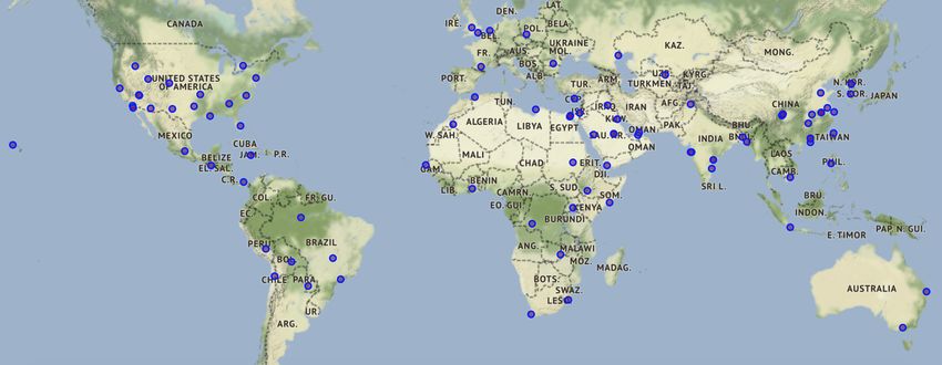
croscopy data present many of the same challenges [38]. in this dataset than past computer vision challenges. When
Lessons learned from this dataset may therefore have broad- comparing the size of annotated instances in the COCO
reaching relevance to the computer vision community. dataset [18], there’s a clear difference in object size dis-
 tributions (see Figure 1A). These smaller objects intrinsi-
2. Related Work cally provide less information as they comprise fewer pix-
 els, making their identification a more difficult task. Finally,
 Past time series computer vision datasets and algorith- the number of instances per image is markedly different in
mic advances have prepared the field to address many of the satellite imagery from the average natural scene dataset (see
problems associated with satellite imagery analysis, allow- Section 3 and Figure 1B). Other data science competitions
ing our dataset to explore additional computer vision prob- have explored datasets with similar object size and density,
lems. The challenge built around the VOT dataset [15] saw particularly in the microscopy domain [21, 11]; however,
impressive results for video object tracking (e.g. [36]), yet those competitions did not address time series applications.
this dataset differs greatly from satellite imagery, with high Taken together, these differences highlight substantial nov-
frame rates and a single object per frame. Other datasets elty for this dataset.
such as MOT17 [17] or MOT20 [6] have multiple targets
of interest, but still have relatively few (< 20) objects per
frame. The Stanford Drone Dataset [23] appears similar 3. Data
at first glance, but has several fundamental differences that The Multi-Temporal Urban Development SpaceNet
result in very different applications. That dataset contains (MUDS) dataset consists of 101 labelled sequences of satel-
overhead videos taken at multiple hertz from a low eleva- lite imagery collected by Planet Labs’ Dove constellation
tion, and typically have ≈ 20 mobile objects (cars, people, between 2017 and 2020, coupled with building footprint la-
buses, bicyclists, etc.) per frame. Because of the high frame bels for every image. The image sequences are sampled at
rate of these datasets, frame-to-frame variation is minimal the 101 distinct areas of interest (AOIs) across the globe,
(see the MOT17 example in Figure 1D). Furthermore, ob- covering six continents (Figure 2). These locations were
jects are larger and less abundant in these datasets than selected to be both geographically diverse and display dra-
buildings are in satellite imagery. As a result, video compe- matic changes in urbanization across a two-year timespan.
titions and models derived therein provide limited insight in
 The MUDS dataset is open sourced under a CC-BY-
how to manage imagery time series with substantial image-
 4.0 ShareAlike International license‡ to encourage broad
to-image variation and overly-dense instance annotations of
 use. This dataset can potentially be useful for many other
target objects. Our data and research will address this gap.
 geospatial computer vision tasks: it can be easily fused
 To our knowledge, no existing dataset has offered a deep
 or augmented with any other data layers that are available
time series of satellite imagery. A number of previous
 through web tile servers. The labels themselves can also
works have studied building extraction from satellite im-
 be applied to any other remote sensing image tiles, such us
agery ([8], [5], [39], [27]), yet these datasets were static.
 high resolution optical or synthetic aperture radar.
The closest comparison is the xView2 challenge and dataset
[10], which examined building damage in satellite image
 3.1. Imagery
pairs acquired before and after natural disasters (i.e. only
two timestamps) in < 20 locations; however, this task fails Images are sourced from Planet’s global monthly
to address the complexities and opportunities posed by anal- basemaps, an archive of on-nadir imagery containing vi-
ysis of deep time series data such as seasonal vegetation and sual RGB bands with a ground sample distance (GSD) (i.e.
lighting changes, or consistent object tracking on a global pixel size) of ≈ 4 meters. A basemap is a reduction of
scale. Other competitions have explored time series data all individual satellite captures (also called scenes) into a
in the form of natural scene video, e.g. object detection spatial grid. These basemaps are created by mosaicing
[6] and segmentation [2] tasks. There are several mean- the best scenes over a calendar month, selected according
ingful dissimilarities between these challenges and the task to quality metrics like image sharpness and cloud cover-
described here. Firstly, frame-to-frame variation is very age. Scenes are stack-ranked with best on top, and spa-
small in video datasets (see Figure 1D). By contrast, the ap- tially harmonized to smoothen scene boundary discontinu-
pearance of satellite images can change dramatically from ities. Monthly basemaps are particularly well suited for the
month to month due to differences in weather, illumination, computer vision analysis of urban growth, since they are rel-
and seasonal effects on the ground, as shown in Figure 1C. atively cloud-free, homogeneous, and represented in a con-
Other time series competitions have used non-imagery data sistent spatio-temporal grid. The monthly cadence is also a
spaced regularly over longer time intervals [9], but none fo- good match to the typical timescale of urban developments.
cused on computer vision tasks.
 The size and density of target objects are very different ‡ https://registry.opendata.aws/spacenet/

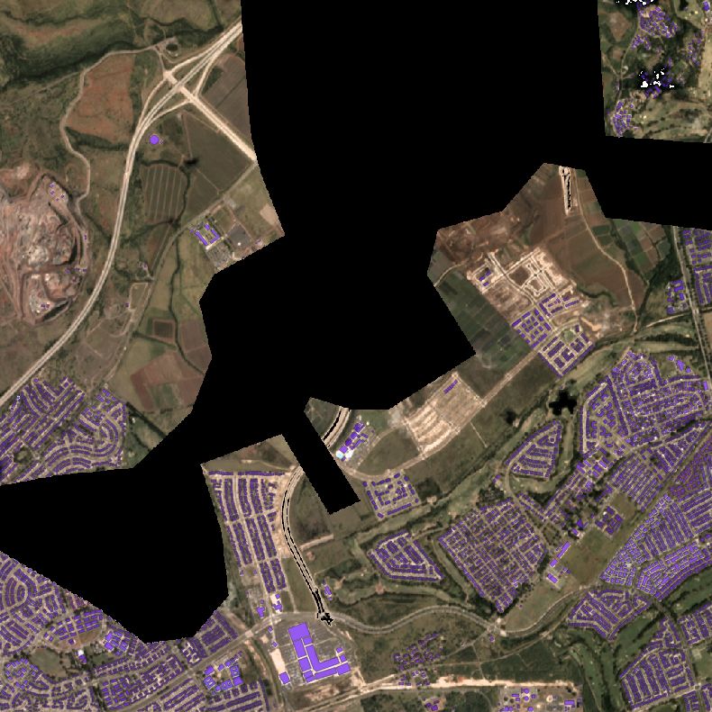
of 18 − 26 months, depending on AOI (median of 24).
 This lengthy time span captures multiple seasons and at-
 mospheric conditions, as well as the commencement and
 completion of multiple construction projects. See Figure 3
 for examples. Images containing an excessive amount of
 clouds or haze were fully excluded from the dataset, thus
 causing minor temporal gaps in some of the time series.

 3.2. Label Statistics
 Each image in the dataset is accompanied by two sets
 of manually created annotations. The first set of labels
 are building footprint polygons defining the outline of each
 building. Each building is assigned a unique identifier (i.e.
 address) that persists throughout the time series. The second
 set of annotations are “unusable data masks” (UDMs) de-
 noting areas of images that are obscured by clouds (see Fig-
 ure 4) or that suffer from image geo-reference errors greater
 than 1 pixel. Geo-referencing is the process of mapping pix-
 els in sensor space to geographic coordinates, performed
 via an empirical fitting procedure that is never exact. In
 rare cases, the scenes that compose the basemaps have spa-
 tial offsets of 5-10 meters. Accounting for such spatial dis-
 placements in the time series would make the modeling task
 significantly harder. Therefore, we decided to eliminate this
 complexity by including these regions in the UDM.
 Each image has between 10 and ≈ 20, 000 building an-
 notations, with a mean of ≈ 4, 600 (the earliest timepoints
Figure 1: A comparison between our dataset and related
 in some geographies have very few buildings completed).
datasets. A. Annotated objects are very small in this dataset.
 This represents much higher label density than natural scene
Plot represents normalized histograms of object size in pix-
 datasets like COCO [18] (Figure 1B), or even overhead
els. Blue is our dataset, red represents all annotations in the
 drone video datasets [34]. As the dataset comprises ≈ 24
COCO 2017 training dataset [18]. B. The density of annota-
 time points at 101 geographic areas, the final dataset in-
tions is very high in our dataset. In each 1024×1024 image,
 cludes > 11M annotations, representing > 500, 000 unique
our dataset has between 10 and over 20,000 objects (mean:
 buildings. (Compare the training data quantities shown for
4,600). By contrast, the COCO 2017 training dataset has at
 other datasets in Table 1.) The building areas vary between
most 50 objects per image. C. Three sequential time points
 approximately 0.25 and 13,000 pixels (median building area
from one geography in our dataset, spanning 3 months of
 of 193 m2 or 12.1 pix2 ), markedly smaller than most labels
development. Compare to D., which displays three sequen-
 in natural scene imagery datasets (Figure 1A).
tial frames in the MOT17 video dataset [17].
 Seasonal effects and weather (i.e. background variation)
 pervade our dataset given the low frame rate of 4 × 10−7 Hz
 (Figure 1C). This “background” change adds to the change
 detection task’s difficulty. This frame-by-frame background
 variation is particularly unique and difficult to recreate via
 simulation or video re-sampling.

 3.3. Labeling Procedure
 We define buildings as static man-made structures where
 Figure 2: Location of MUDS data cubes. an individual could take shelter, with no minimum footprint
 size. The uniqueness of the dataset presents distinct label-
 The size of each image is 1024 × 1024 pixels, corre- ing challenges. First, small buildings can be under-resolved
sponding to ≈ 18 km2 , and the total area of the images to the human eye in a given image, making it difficult to
in the dataset is 41, 250 km2 . See Table 1 or spacenet.ai locate and discern from other non-building structures. Sec-
for additional statistics. The time series contain imagery ond, in locations undergoing building construction, it can

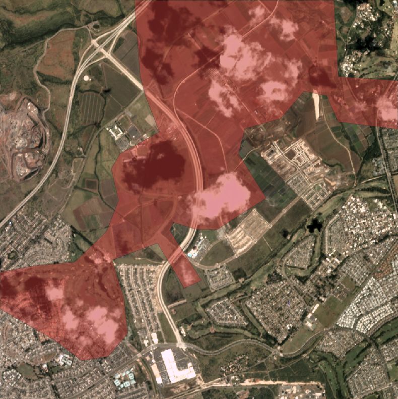
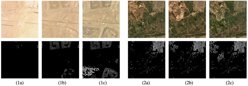
Figure 3: Time series of two data cubes. Left column (e.g. 1a) denotes the start of the times series, the middle column (e.g.
1b) the approximate midpoint, and the right column (e.g. 1c) shows the final image. The top row displays imagery, while the
bottom row illustrates the labeled building footprints.

 Table 1: Comparison of Selected Time Series Datasets
 MUDS VOT-ST2020 MOT20 Stanford Drone DAVIS 2017 YouTube-VOS
 Property [14] [6] [23] [3] [41]
 Scenes 101 60 4 60 90 4,453
 Total Frames 2,389 19,945 8,931 522,497 6,208 ∼603,000
 Unique Tracks 538,073 60 2,332 10,300 216 7,755
 Total Labels 11,079,262 19,945 1,652,040 10,616,256 13,543 197,272
 Median Frames/Scene 24 257.5 1,544 11,008 70.5 ∼135 (mean)
 Ground Sample Dist. 4.0m n/a n/a ∼2cm n/a n/a
 Frame Rate 1/month 30fps 25fps 30fps 20fps 30fps (6fps labels)
 Annotation Polygon Seg. Mask BBox BBox Seg. Mask Seg. Mask
 Objects Buildings Various Pedestrians, Pedestrians & Various Various
 etc. Vehicles

be difficult to determine what point in time the structure be- Once one type of such ephemeral structures is identified as
comes a building per our definition. Third, variability in a confusion source, all other similar structures are also ex-
image quality, atmospheric conditions, shadows, and sea- cluded (Figure 5). Labeling took 7 months by a team of 5;
sonal phenology can introduce additional confusion. Mit- each data cube was annotated by one person, reviewed and
igating these complexities and minimizing label noise was corrected by another, with final validation by the team lead.
of paramount importance, especially along the temporal di- Annotators also used a privately-licensed high resolution
mension. Even though the dataset AOIs were selected to imagery map to help discriminate uncertain cases. This high
contain urban change, construction events are still highly resolution map is useful to gain contextual information of
imbalanced compared to the full spatio-temporal volume. the region and to guide the precise building outlines that
Thus, temporal consistency was a fundamental area of focus are unclear from the dataset imagery alone. Once a build-
in the labeling strategy. In cases of high uncertainty with a ing candidate was identified in the MUDS imagery, the high
particular building candidate, annotators examined the full resolution map was used to confirm the building geometry.
time series to gain temporal and contextual information of In other words, labels were not created on the high resolu-
the precise location. For example, a shadow from a neigh- tion imagery first. While the option of labeling on high res-
boring structure might be confused as a building, but this olution might seem attractive, it poses labeling risks such as
becomes evident when inspecting the full data cube. Tem- capturing buildings that are not visible at all in the MUDS
poral context can also help identify groups of objects. Some imagery. In addition, the high resolution map is static and
regions have structures that resemble buildings in a given composed of imagery acquired over a long range of dates,
image, but are highly variable in time. Objects that appear thus making it difficult to perform temporal comparisons
and disappear multiple times are unlikely to be buildings. between this map and the dataset imagery.

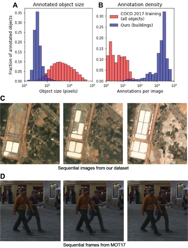
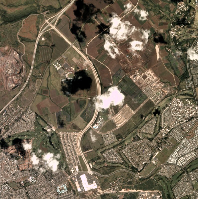
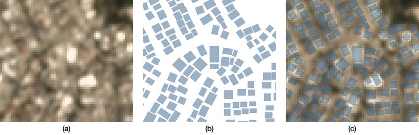
Figure 6: Zoom in of one particularly dense region illustrat-
 ing the very high fidelity of labels. (a) Raw image. (b) Foot-
 print polygon labels. (c) Footprints overlaid on imagery.
 (a) Raw Image (b) UDM overlaid

 2. Copy all the building labels onto the next image (not
 the UDM). Examine carefully all buildings in the new
 image, and edit the labels with any changes. Edits are
 only be made when there is significant confidence that
 a building appeared or disappeared. If a new build-
 ing appeared, assign a new unique identifier. Toggle
 through multiple images in the time series to ensure:
 (a) there is a true building change and (b) that it is ap-
 plied to the correct time point. Also, create a UDM.
 (c) Masked image + labels (d) Zoomed labels
 3. Repeat step 2 for the remaining time points.
Figure 4: Single image in a data cube. (a) Image with cloud
cover. (b) Image with UDM overlaid. (c) Masked image This process attempts to enforce temporal consistency
with building labels overlaid. (d) Zoom showing the high and reduce object confusion. While label noise is appre-
fidelity of building labels. ciable in small objects, the use of high resolution imagery
 to label results in labels of significantly higher fidelity that
 would be achievable from the Planet data alone, as illus-
 trated in Figure 6. This “omniscient labeling” is one of the
 key features of the MUDS dataset. We will show in Sec-
 tion 5 that the baseline algorithm does a surprisingly good
 job of extracting high-resolution features from the medium-
 resolution imagery. In effect, the labels are encoding infor-
 mation that is not visible to humans in the imagery, which
Figure 5: Example of how temporal context can help with the baseline algorithm is able to capitalize upon.
object identification. If the middle image were to be la-
beled in isolation, objects A and B could be annotated as 4. Evaluation Metrics
buildings. However, taking into account the adjacent im-
ages, these objects exist only for one month and therefore To evaluate model performance on a time series of
are unlikely to be buildings. Object C is also unlikely to be identifier-tagged footprints such as MUDS, we introduce a
a building, just by group association. new evaluation metric: the SpaceNet Change and Object
 Tracking (SCOT) metric [13]. As discussed later, existing
 metrics have a number of shortcomings that are addressed
 The procedure to annotate each time series can be sum-
 by SCOT. The SCOT metric combines two terms: a track-
marized as follows:
 ing term and a change detection term. The tracking term
 1. Start with the first image in the series. Identify the evaluates how often a proposal correctly tracks the same
 location of all visible structures. If the building lo- buildings from month to month with consistent identifier
 cation and outline are clear, draw a polygon around numbers. In other words, it measures the model’s ability
 it. Otherwise, overlay a high resolution optical map to characterize what stays the same as time goes by. The
 to help confirm the presence of the building and draw change detection term evaluates how often a proposal cor-
 the outline. Assign a unique integer identifier to each rectly picks up on the construction of new buildings. In
 building. In addition, identify any regions in the im- other words, it measures the model’s ability to characterize
 age with impaired ground visibility or defects and add what changes as time goes by.
 their polygons to the UDM layer of this image. For both terms, the calculation starts the same way: find-

Location Location
ing “matches” between ground truth building footprints and
proposal building footprints for each month. A pair of foot-

 Time
 11

 Time
 January 1 3 January 11
 1 3

prints (one ground truth and one proposal) are eligible to be February 1 2
 12
 3
 11
 13

 February 1 2
 12
 3
 11
 13

matched if their intersection over union (IOU) exceeds 0.25, March 1 2
 12
 3 4
 13
 March
 12
 4
 13
 1 2 3

and no footprint may be matched more than once. We se- April 1
 12
 2
 14
 12 14
 April 1 2
lect an IOU of 0.25 to mimic Equation 5 of ImageNet [25]), May
 12 14
 11 4
 15
 12 14
 11
 15
 1 2 3 May 4
 1 2 3
which sets IOU < 0.5 for small objects. A set of matches
is chosen that maximizes the number of matches. If there is !"#$% = !
 &
 &'" (')
 = 0.593
 Match that is not a mismatch
 !"#$%& = !
 '
 = 0.333
 New buildings only
 '(" )('
 Mismatch Unmatched
more than one way to achieve that maximum, then as a tie- proposal
 New proposal IDs only

breaker the set with the largest sum of IOUs is used. This is (a) Tracking Term (b) Change Term
an example of the unbalanced linear assignment problem in
combinatorics. Figure 7: (a) Example of SCOT metric tracking term. Solid
 If model performance were being evaluated for a sin- brown polygons are ground truth building footprints, and
gle image (instead of a time series), a customary next step outlines are proposal footprints. Each footprint’s corre-
might be calculating an F1 score, where matches are con- sponding identifier number is shown. (b) Example of SCOT
sidered true positives (tp) and unmatched ground truth and metric change detection term, using the same set of ground
proposal footprints are considered false negatives (f n) and truth and proposal footprints. This term ignores all ground
false positives (f p) respectively. truth and proposal footprints with previously-seen identi-
 fiers, which are indicated in a faded-out gray color.
 tp
 F1 = (1)
 tp + 12 (f p + f n)
 One important property of this term is that a set of static
 The tracking term and change detection term both gen- proposals that do not vary from one month to another will
eralize this to a time series, each in a different way. receive a change detection term of 0, even for a time series
 The tracking term penalizes inconsistent identifiers with very little new construction. (In the MUDS dataset,
across time steps. A match is considered a “mismatch” the construction of new buildings is by far the most com-
if the ground truth footprint’s identifier was most recently mon change; the metric could be generalized to accommo-
matched to a different proposal ID, or vice versa. For the date building demolition or other changes by any of several
purpose of the tracking term, mismatches (mm) are not straightforward generalizations.)
counted as true positives. So each mismatch decreases the To compute the final score, the two terms are combined
number of true positives by one. This effectively divorces with a weighted harmonic mean:
the ground truth footprint from its mismatched proposal
footprint, creating an additional false negative and an ad- Fchange · Ftrack
ditional false positive. That amounts to the following trans- Fscot = (1 + β 2 ) (5)
 β 2 Fchange + Ftrack
formations:
 We use a value of β = 2 to emphasize the part of the task
 tp → tp − mm
 (tracking) that has been less commonly explored in an over-
 f p → f p + mm (2) head imagery context. For a dataset like MUDS with multi-
 f n → f n + mm ple AOIs, the overall SCOT score is the arithmetic mean of
 the scores of the individual AOIs.
Applying these to the F1 expression above gives the formula Figure 7a is a cartoon example of calculating the tracking
for the tracking term: term on a row of four buildings imaged over five months
 tp − mm (during which time two of the four are newly-constructed,
 Ftrack = (3) and two are temporarily occluded by clouds). Figure 7b
 tp + 12 (f p + f n)
 illustrates the change detection term for the same case.
 The second term in the SCOT metric, the change detec- For geospatial work, the SCOT metric has a number
tion term, incorporates only new footprints. That is, ground of advantages over evaluation metrics developed for object
truth or proposal footprints with identifier numbers making tracking in video, such as the Multiple Object Tracking Ac-
their first chronological appearance. Letting the subscript curacy (MOTA) metric [1]. MOTA scores are mathemati-
new indicate the count of tp’s, f p’s, and f n’s that persist cally unbounded, making them less intuitively interpretable
after dropping non-new footprints: for challenging low-score scenarios, and sometimes even
 yielding negative scores. More critically, for scenes with
 tpnew only a small amount of new construction, it’s possible to
 Fchange = 1 (4)
 tpnew + 2 (f pnew + f nnew ) achieve a high MOTA score with a set of proposal footprints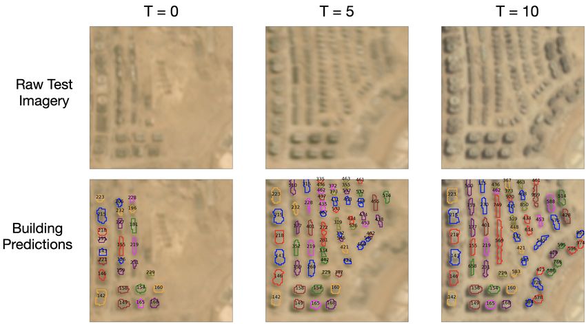

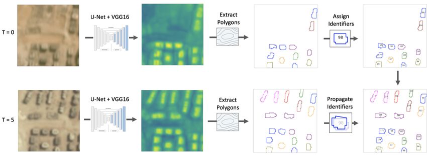
that shows no time-dependence whatsoever. Since under-
standing time-dependence is usually a primary purpose of
time series data, this is a serious drawback. SCOT’s change
detection term prevents this. In fact, many such approaches
to “gaming” the SCOT metric by artificially increasing one
term will decrease the other term, leaving no obvious alter-
native to intuitively-better model performance as a way to
raise scores.
 Figure 8: Baseline algorithm for building footprint extrac-
5. Experiments tion and identifier tracking showing evolution from T = 0
 (top row) to T = 5 (bottom row). The input image is fed
 For object tracking, one could in theory leverage the re- into our segmentation model, yielding a building mask (sec-
sults of previous challenges (e.g. MOT20 [6]), yet the sig- ond column). This mask is refined into building footprints
nificant differences between MUDS and previous datasets (third column), and unique identifiers are allocated (right
such as high density and small object size (see Figure 1) column).
render previous approaches unsuitable. For example, ap-
proaches such as TrackR-CNN [35] are untrainable as each
instance requires a separate channel resulting in a mem-
ory explosion for images with many thousands of objects.
Other approaches such as Joint Detection and Embedding
(JDE) [37] are trainable; however inference results are ul-
timately incoherent due to the tiny object size and density
overwhelming the YOLOv3 [22] detection grid. Despite
these challenges, the spatially static nature of our objects of
interest somewhat simplifies tracking objects between each
observation. Consequently, this dataset should incentivize
the development of new object tracking algorithms that can
cope with a lack of resolution, spatial stasis, minimal size,
and dense clustering of objects. Figure 9: Example tracking performance of the baseline
 As a result of the challenges listed above, we choose to algorithm. Note that larger, well-separated buildings are
experiment with semantic segmentation based approaches tracked well between epochs, while denser regions are more
to detect and track buildings over time. These methods are challenging for tracking.
adapted from prize winning approaches for the SpaceNet
4 and 6 Building Footprint Extraction Challenges [40, 28]. Table 2: Building Tracking Performance
Our architecture comprises a U-Net [24] with different en-
coders. The first “baseline” approach uses a VGG16 [30] Approach
 Metric
 VGG-16 EfficentNet
encoder and a custom loss function of L = J + 4 · BCE,
 F1 (IOU ≥ 0.25) 0.45 ± 0.13 0.42 ± 0.12
where J is Jaccard distance and BCE denotes binary
 Tracking Score 0.40 ± 0.10 0.39 ± 0.10
cross entropy. The second approach uses a more advanced Change Score 0.06 ± 0.05 0.07 ± 0.05
EfficientNet-B5 [32] encoder with a loss of L = F + D SCOT 0.17 ± 0.10 0.18 ± 0.09
where F is Focal loss [19] and D is Dice loss.
 To ensure robust testing statistics, we train the model on
60 data cubes, testing on the remaining 41 data cubes. We Matched footprintes are assigned the same identifier as the
train the segmentation models with an Adam optimizer on previous timestep, while footprints without significant over-
the 1424 images of the training set for 300 epochs and a lap with preceding geometries are assigned a new unique
learning rate of 10−4 (baseline) or 100 epochs and a learn- identifier. The baseline algorithm is illustrated in Figure
ing rate of 2 × 10−4 (EfficentNet). 8; note that building identifiers are well matched between
 At inference time binary building prediction masks are epochs. Performance is summarized in Table 2. For scoring
converted to instance segmentations of building footprints. we assess only buildings with area ≥ 4 px2 .
Each footprint at t = 0 is assigned a unique identifier. Localizing and tracking buildings in medium resolu-
For each subsequent time step building footprints polygons tion (≈ 4m) imagery is quite challenging, but surpris-
are compared to the positions of the previous time step. ingly achievable in our experiments. For well separated
Building identifier matching is achieved by an optimized buildings, building localization and tracking performs fairly
matching of polygons with a minimum IOU overlap of 0.25. well; for example in Figure 9) we find a localization F1

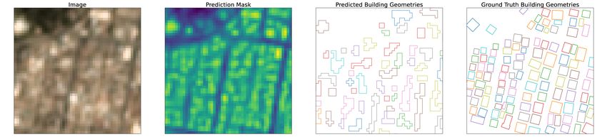
of 1.2 meters objects have an average extent of 4.4 pixels.
 The average building area for the MUDS dataset is 332
 m2 , implying an extent of 18.2 m for a square object. For
 a 4 meter resolution, this gives an average extent of 4.5
 pixels, comparable to the 4.4 pixel extent of xView. The
Figure 10: Prediction in a difficult, crowded region. De- observed MUDS F1 score of 0.45 is within error bars of
spite the inherent difficulties in separating nearby buildings the results of the xView results, see Table 3. Of particu-
at medium resolution, for this image F1 = 0.40. lar note is that while the F1 scores and object pixel sizes of
 Table 3 are comparable, the datasets stem from vastly differ-
score of 0.55, and a SCOT score of 0.31. For dense regions, ent sensors, and the techniques are wildly different as well
building tracking is far more difficult; in Figure 10 we still (a Googlenet-based object detection architecture versus a
see decent performance in building localization (F1 = 0.40), VGG16-based segmentation architecture). Apparently, ob-
yet building tracking and change detection is very chal- ject detection performance holds across sensors and algo-
lenging (SCOT = 0.07) since inter-epoch footprints overlap rithms as long as object pixel sizes are comparable.
poorly. The change term of SCOT is particularly challeng-
ing, as correctly identifying the origin epoch of each build- Table 3: F1 Performance Across Datasets
ing is non-trivial, and spurious proposals are also penalized.
 Dataset GSD (m) Object Size (pix) F1
 In an attempt to raise the scores of Table 2, we also en-
 xView 1.2 4.4 0.41 ± 0.03
deavor to incorporate the time dimension into training. As
 MUDS 4.0 4.5 0.45 ± 0.13
previously mentioned, existing approaches transfer poorly
to this dataset, so we attempt a simple approach of stacking
multiple images at training time. For each date we train on
the imagery for that date plus the four chronologically ad- 7. Conclusions
jacent future observations [t = 0, t + 1, t + 2, t + 3, t + 4]
for five total dates of imagery. When the number of remain- The Multi-temporal Urban Development SpaceNet
ing observations in the time series becomes less than five, (MUDS, also known as SpaceNet 7) dataset is a newly
we repeatedly append the final image for each area of in- developed corpus of imagery and precise labels designed
terest. We find no improvement with this approach (SCOT for tracking building footprints and unique identifiers. The
= 0.17 ± 0.08). dataset covers over 100 locations across 6 continents, with
 We also note no significant difference in scores between a deep temporal stack of 24 monthly images and over
the VGG-16 and EfficentNet architectures (Table 2), imply- 11,000,000 labeled objects. The significant scene-to-scene
ing that older architectures are essentially as adept as state- variation of the monthly images poses a challenge for com-
of-the-art architectures when it comes to extracting infor- puter vision algorithms, but also raises the prospect of
mation from the small objects in this dataset. developing algorithms that are robust to seasonal change
 While not fully explored here, we also anticipate that and atmospheric conditions. One of the key characteris-
researchers may improve upon the baseline using models tics of the MUDS dataset is exhaustive “omniscient label-
specifically intended for time series analysis (e.g. Recurrent ing” with labels precision far exceeding the base imagery
Neural Networks (RNNs) [20] and Long-Short Term Mem- resolution of 4 meters. Such dense labels present signifi-
ory networks (LSTMs) [12]. In addition, numerous “classi- cant challenges in crowded urban environments, though we
cal” geospatial time series methods exist (e.g. [42]) which demonstrate surprisingly good building extraction, tracking,
researchers may find valuable to incorporate into their anal- and change detection performance with our baseline algo-
ysis pipelines as well. rithm. Intriguingly, our object detection performance of
 F 1 = 0.45 for objects averaging 4-5 pixels in extent is con-
6. Discussion sistent with previous object detection studies, even though
 these studies used far different algorithmic techniques and
 Intriguingly, the score of F 1 = 0.45 for our baseline datasets. There are numerous avenues of research beyond
mode parallels previous results observed in overhead im- the scope of this paper that we hope the community will
agery. [29] studied object detection performance in xView tackle with this dataset: the efficacy of super-resolution,
[16] satellite imagery for various resolutions and five dif- adapting video time-series techniques to the unique features
ferent object classes. These authors used the YOLT [33] of MUDS, experimenting with RNNs, Siamese networks,
object detection framework, which uses a custom network LSTMs, etc. Furthermore, the dataset has the potential to
based on the Googlenet [31] architecture. The mean extent aid a number of humanitarian efforts connected with popu-
of the objects in this paper was 5.3 meters; at a resolution lation dynamics and UN sustainable development goals.

References Porikli, and Luka Čehovin. A novel performance evaluation
 methodology for single-target trackers. IEEE Transactions
 [1] Keni Bernardin, Alexander Elbs, and Rainer Stiefelhagen. on Pattern Analysis and Machine Intelligence, 38(11):2137–
 Multiple object tracking performance metrics and evalua- 2155, Nov 2016. 2
 tion in a smart room environment. Sixth IEEE International
 [16] Darius Lam, Richard Kuzma, Kevin McGee, Samuel Doo-
 Workshop on Visual Surveillance, in conjunction with ECCV,
 ley, Michael Laielli, Matthew Klaric, Yaroslav Bulatov, and
 2006. 6
 Brendan McCord. xview: Objects in context in overhead
 [2] Sergi Caelles, Jordi Pont-Tuset, Federico Perazzi, Alberto imagery. CoRR, abs/1802.07856, 2018. 8
 Montes, Kevis-Kokitsi Maninis, and Luc Van Gool. The
 [17] Laura Leal-Taixé, Anton Milan, Konrad Schindler, Daniel
 2019 davis challenge on vos: Unsupervised multi-object seg-
 Cremers, Ian D. Reid, and Stefan Roth. Tracking the track-
 mentation. arXiv:1905.00737, 2019. 2
 ers: An analysis of the state of the art in multiple object
 [3] Sergi Caelles, Jordi Pont-Tuset, Federico Perazzi, Alberto tracking. CoRR, abs/1704.02781, 2017. 2, 3
 Montes, Kevis-Kokitsi Maninis, and Luc Van Gool. The [18] Tsung-Yi Lin, Michael Maire, Serge J. Belongie, Lubomir D.
 2019 DAVIS challenge on VOS: Unsupervised multi-object Bourdev, Ross B. Girshick, James Hays, Pietro Perona, Deva
 segmentation. arXiv:1905.00737, 2019. 4 Ramanan, Piotr Dollár, and C. Lawrence Zitnick. Microsoft
 [4] Simiao Chen, Michael Kuhn, Klaus Prettner, and David E. COCO: common objects in context. CoRR, abs/1405.0312,
 Bloom. The global macroeconomic burden of road injuries: 2014. 2, 3
 estimates and projections for 166 countries. 2019. 1 [19] Tsung-Yi Lin, Priya Goyal, Ross Girshick, Kaiming He, and
 [5] Ilke Demir, Krzysztof Koperski, David Lindenbaum, Guan Piotr Dollár. Focal loss for dense object detection. In Pro-
 Pang, Jing Huang, Saikat Basu, Forest Hughes, Devis Tuia, ceedings of the IEEE international conference on computer
 and Ramesh Raskar. Deepglobe 2018: A challenge to parse vision, pages 2980–2988, 2017. 7
 the earth through satellite images. In Proceedings of the [20] Tomáš Mikolov, Martin Karafiát, Lukáš Burget, Jan
 IEEE Conference on Computer Vision and Pattern Recog- Černocký, and Sanjeev Khudanpur. Recurrent neural net-
 nition (CVPR) Workshops, June 2018. 2 work based language model. In Proceedings of the 11th An-
 [6] Patrick Dendorfer, Hamid Rezatofighi, Anton Milan, Javen nual Conference of the International Speech Communication
 Shi, Daniel Cremers, Ian Reid, Stefan Roth, Konrad Association (INTERSPEECH 2010), 2010. 8
 Schindler, and Laura Leal-Taixé. MOT20: A benchmark for [21] Recursion Pharmaceuticals. Cellsignal: Disentangling bio-
 multi object tracking in crowded scenes, 2020. 2, 4, 7 logical signal from experimental noise in cellular images. 2
 [7] R. Engstrom, D. Newhouse, and V. Soundararajan. Estimat- [22] Joseph Redmon and Ali Farhadi. Yolov3: An incremental
 ing small area population density using survey data and satel- improvement. arXiv preprint arXiv:1804.02767, 2018. 7
 lite imagery: An application to sri lanka. Urban Economics
 [23] Alexandre Robicquet, Amir Sadeghian, Alexandre Alahi,
 & Regional Studies eJournal, 2019. 1
 and Silvio Savarese. Learning social etiquette: Human tra-
 [8] Adam Van Etten, Dave Lindenbaum, and Todd M. Bacas- jectory understanding in crowded scenes. In ECCV, 2016. 2,
 tow. Spacenet: A remote sensing dataset and challenge se- 4
 ries. CoRR, abs/1807.01232, 2018. 2
 [24] Olaf Ronneberger, Philipp Fischer, and Thomas Brox. U-
 [9] Google. Web traffic time series forecasting: Forecast future net: Convolutional networks for biomedical image segmen-
 traffic to wikipedia pages. 2 tation. In Proceedings of the 2015 International Conference
[10] Ritwik Gupta, Richard Hosfelt, Sandra Sajeev, Nirav Patel, on Medical Image Computing and Computer-Assisted Inter-
 Bryce Goodman, Jigar Doshi, Eric Heim, Howie Choset, vention, 2015. 7
 and Matthew Gaston. Creating xbd: A dataset for assessing [25] Olga Russakovsky, Jia Deng, Hao Su, Jonathan Krause, San-
 building damage from satellite imagery. In Proceedings of jeev Satheesh, Sean Ma, Zhiheng Huang, Andrej Karpathy,
 the 2019 CVF Conference on Computer Vision and Pattern Aditya Khosla, Michael S. Bernstein, Alexander C. Berg,
 Recognition Workshops, 2019. 2 and Fei-Fei Li. Imagenet large scale visual recognition chal-
[11] Booz Allen Hamilton and Kaggle. Data science bowl 2018: lenge. CoRR, abs/1409.0575, 2014. 6
 Spot nuclei. speed cures. 2 [26] Nadine Schuurman, Robert S. Fiedler, Stefan C.W. Grzy-
[12] Sepp Hochreiter and Jurgen Schmidhuber. Long short-term bowski, and Darrin Grund. Defining rational hospital catch-
 memory. Neural Computation, 9, 1997. 8 ments for non-urban areas based on travel time. 5, 2006. 1
[13] Daniel Hogan and Adam Van Etten. The SpaceNet change [27] Jacob Shermeyer, Daniel Hogan, Jason Brown, Adam
 and object tracking (SCOT) metric, August 2020. 5 Van Etten, Nicholas Weir, Fabio Pacifici, Ronny Hansch,
[14] Matej Kristan, Ales Leonardis, Jiri Matas, Michael Fels- Alexei Bastidas, Scott Soenen, Todd Bacastow, and Ryan
 berg, Roman Pflugfelder, Joni-Kristian Kamarainen, Luka Lewis. Spacenet 6: Multi-sensor all weather mapping
 Čehovin Zajc, Martin Danelljan, Alan Lukezic, Ondrej Dr- dataset. In Proceedings of the IEEE/CVF Conference on
 bohlav, Linbo He, Yushan Zhang, Song Yan, Jinyu Yang, Computer Vision and Pattern Recognition (CVPR) Work-
 Gustavo Fernandez, et al. The eighth visual object tracking shops, June 2020. 2
 VOT2020 challenge results, 2020. 4 [28] Jacob Shermeyer, Daniel Hogan, Jason Brown, Adam
[15] Matej Kristan, Jiri Matas, Aleš Leonardis, Tomas Vojir, Ro- Van Etten, Nicholas Weir, Fabio Pacifici, Ronny Hansch,
 man Pflugfelder, Gustavo Fernandez, Georg Nebehay, Fatih Alexei Bastidas, Scott Soenen, Todd Bacastow, and Ryan

Lewis. Spacenet 6: Multi-sensor all weather mapping [42] Zhe Zhu. Change detection using landsat time series: A re-
 dataset. In Proceedings of the IEEE/CVF Conference on view of frequencies, preprocessing, algorithms, and applica-
 Computer Vision and Pattern Recognition (CVPR) Work- tions. ISPRS Journal of Photogrammetry and Remote Sens-
 shops, June 2020. 7 ing, 130:370 – 384, 2017. 8
[29] Jacob Shermeyer and Adam Van Etten. The effects of super-
 resolution on object detection performance in satellite im-
 agery. In Proceedings of the IEEE/CVF Conference on Com-
 puter Vision and Pattern Recognition (CVPR) Workshops,
 June 2019. 8
[30] Karen Simonyan and Andrew Zisserman. Very deep convo-
 lutional networks for large-scale image recognition. In Pro-
 ceeings of the 2015 International Conference on Learning
 Representations, 2015. 7
[31] C. Szegedy, Wei Liu, Yangqing Jia, P. Sermanet, S. Reed,
 D. Anguelov, D. Erhan, V. Vanhoucke, and A. Rabinovich.
 Going deeper with convolutions. In 2015 IEEE Conference
 on Computer Vision and Pattern Recognition (CVPR), pages
 1–9, 2015. 8
[32] Mingxing Tan and Quoc V. Le. Efficientnet: Rethinking
 model scaling for convolutional neural networks, 2020. 7
[33] A. Van Etten. Satellite imagery multiscale rapid detection
 with windowed networks. In 2019 IEEE Winter Conference
 on Applications of Computer Vision (WACV), pages 735–
 743, 2019. 8
[34] Stanford Computational Vision and Geometry Lab. Stanford
 drone dataset. 3
[35] Paul Voigtlaender, Michael Krause, Aljosa Osep, Jonathon
 Luiten, Berin Balachandar Gnana Sekar, Andreas Geiger,
 and Bastian Leibe. MOTS: Multi-object tracking and seg-
 mentation, 2019. 7
[36] Qiang Wang, Li Zhang, Luca Bertinetto, Weiming Hu, and
 Philip H.S. Torr. Fast online object tracking and segmenta-
 tion: A unifying approach. In The IEEE Conference on Com-
 puter Vision and Pattern Recognition (CVPR), June 2019. 2
[37] Zhongdao Wang, Liang Zheng, Yixuan Liu, Yali Li, and
 Shengjin Wang. Towards real-time multi-object tracking,
 2020. 7
[38] Nicholas Weir, JJ Ben-Joseph, and Dylan George. Viewing
 the world through a straw: How lessons from computer vi-
 sion applications in geo will impact bio image analysis, Jan
 2020. 2
[39] Nicholas Weir, David Lindenbaum, Alexei Bastidas,
 Adam Van Etten, Sean McPherson, Jacob Shermeyer, Varun
 Kumar, and Hanlin Tang. Spacenet mvoi: A multi-view over-
 head imagery dataset. In Proceedings of the IEEE/CVF In-
 ternational Conference on Computer Vision (ICCV), October
 2019. 2
[40] Nicholas Weir, David Lindenbaum, Alexei Bastidas,
 Adam Van Etten, Sean McPherson, Jacob Shermeyer,
 Varun Kumar Vijay, and Hanlin Tang. Spacenet MVOI: a
 multi-view overhead imagery dataset. In Proceedings of the
 2019 International Conference on Computer Vision, volume
 abs/1903.12239, 2019. 7
[41] Ning Xu, Linjie Yang, Yuchen Fan, Dingcheng Yue, Yuchen
 Liang, Jianchao Yang, and Thomas Huang. YouTube-VOS:
 A large-scale video object segmentation benchmark, 2018. 4