Learning the Lantern: Neural network applications to broadband photonic lantern modelling
←
→
Page content transcription
If your browser does not render page correctly, please read the page content below
Learning the Lantern: Neural network applications to broadband
                                                  photonic lantern modelling

                                                  David Sweeneya, b, * , Barnaby R. M. Norrisa, b , Peter Tuthilla, b , Richard Scalzoc , Jin Weia, b ,
                                                  Christopher H. Bettersa, b , Sergio G. Leon-Savala, b
                                                  a
                                                    The University of Sydney, Faculty of Science, School of Physics, Physics Road, Sydney, Australia, 2006
                                                  b
                                                    Sydney Astrophotonic Instrumentation Laboratories, Physics Road, Sydney, Australia, 2006
                                                  c
                                                    The University of Sydney, Faculty of Science, School of Mathematics & Statistics, Physics Road, Sydney, Australia,
arXiv:2108.13274v1 [physics.optics] 30 Aug 2021

                                                  2006

                                                  Abstract. Photonic lanterns allow the decomposition of highly multimodal light into a simplified modal basis such
                                                  as single-moded and/or few-moded. They are increasingly finding uses in astronomy, optics and telecommunications.
                                                  Calculating propagation through a photonic lantern using traditional algorithms takes ∼ 1 hour per simulation on
                                                  a modern CPU. This paper demonstrates that neural networks can bridge the disparate opto-electronic systems, and
                                                  when trained can achieve a speed-up of over 5 orders of magnitude. We show that this approach can be used to
                                                  model photonic lanterns with manufacturing defects as well as successfully generalising to polychromatic data. We
                                                  demonstrate two uses of these neural network models, propagating seeing through the photonic lantern as well as
                                                  performing global optimisation for purposes such as photonic lantern funnels and photonic lantern nullers.

                                                  Keywords: astrophotonics, optical fibres, adaptive optics, photonic lantern, neural network, broadband modelling.

                                                  *Corresponding author, david.sweeney@sydney.edu.au

                                                  1 Introduction
                                                  Photonic lanterns (PLs)1 are increasingly important devices finding use in fields such as astronomy,
                                                  for wavefront sensing2 and transforming astronomical signals;3–5 in optics, for reducing modal
                                                  noise,6 amplification7 and beam shaping;8 and in telecommunications, for free space communi-
                                                  cation through the atmosphere9 and spatial division multiplexing.10–15 Of particular astronomical
                                                  interest is the use of PLs to efficiently couple seeing-affected light into single mode fibres for
                                                  single-mode spectroscopy applications,16–18 including recent on-sky tests.19, 20
                                                      Hampering this widespread interest, traditional numerical beam propagation algorithms (such
                                                  as RSoft’s BeamPROP) are only capable of calculating propagation through a three dimensional
                                                  PL in ∼ 1 hour per simulation on a contemporary quad-core CPU (we state time per quad-core
                                                  here as a useful metric since virtually all modern CPUs are built around a quad-core design). These
                                                  beam propagation algorithms solve Maxwell’s equations at each point of a fine grid, interspersed
                                                  through the medium. This is too slow for many applications, putting the realistic simulation of
                                                  a PL’s response to atmospheric-seeing time sequences well out of reach, particularly for poly-
                                                  chromatic data, and prevents the performing of global optimisations, e.g. to find a specific input
                                                  wavefront for a given output criteria. In this latter case, basin-hopping gradient descent (or some
                                                  other optimisation algorithm) can be deployed to use the PL for novel applications like PL funnels
                                                  and PL nullers. The inability of traditional beam propagation algorithms to rapidly simulate PLs
                                                  motivates our use of neural networks (NN) as a faster alternative.

                                                                                                           1
A fundamental challenge is that the relationship between the wavefront at a PL’s input and the
measured intensities at its output is non-linear (since the intensity is the square of the complex
electric field). NNs are thus extremely valuable to model this since they can be truly non-linear.
Across many fields, NNs are rising to prominence for their ability to approximate arbitrary, non-
linear functions. Buoyed by the large data sets and increasing computing power which charac-
terises modern machine learning problems, NNs now outperform many classic approaches for a
wide variety of problems.21–24
    Here, we explore the deployment of deep learning to synthesise these elements, achieving a
speed-up compared to traditional beam propagation algorithm of greater than 5 orders of mag-
nitude. Another key advantage of this approach is that the model can be built from in-situ test
measurements (‘training data’) of a real PL. These measurements include the effects caused by the
manufacturing defects and an imperfect optical injection system, rather than the idealised parame-
ters used to create an RSoft model. Alternatively the training data can be initially produced from
test-propagations through a conventional beam-propagation algorithm. Moreover, it generalises to
broadband data and is able to deliver accurate predictions for untrained wavelengths. We demon-
strate the case of starlight distorted by natural astronomical seeing passing through a PL, with only
tens of milliseconds of compute time per simulation. Furthermore, two applications discussed be-
low that would formerly have required substantial resources are now straightforward with this new
capability.

1.1 Photonic Lanterns

Fig 1 A diagram of a PL depicting the splitting of modes from one multimode optical fibre to a number of individual
single-mode optical fibres.

   PLs are composed of a multimode optical fibre section which adiabatically transitions into
many single-mode optical fibres, as shown in Fig. 1. Light incident on the multimode optical

                                                        2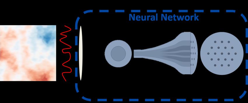
fibre propagates through the multimodal region before gradually transitioning into an array of
single-mode fibres—with higher refractive index—which increase in diameter in this direction of
propagation. Light propagating through the allowed modes of the lantern is thus distributed, in
varying fluxes, among the array of single-mode fibres.25 In order to conserve flux, the number of
outputs must equal the number of modes in the multimode optical fibre. The phase and intensity
of the output of each single-mode fibre encodes the information present in the original multimode
field, up to the complexity allowed by the modes supported by the multimode region.2 If a suitable
model of the PL existed, then by measuring the incident multimode field it would be possible to
determine the output intensities of each single-mode fibre.
    Calculating the intensities of the array of single-mode fibres to any given multi-mode input
field is non-trivial. For an analytic solution of a physical PL, the coupling coefficients must be
determined experimentally—they cannot be precisely specified during the design due to imperfec-
tions in the fabrication process. For a photonic device, such as a 19 core hexagonally packed PL
each with a changing cross section along the length, determination of the coupling coefficients is
not straightforward—even using coupled-mode theory with nearest neighbour approximations. We
demonstrate, in Sec. 4.1 that machine learning techniques can be formulated into a system able to
learn and predict a lantern’s transfer function when trained on the lantern’s response to a set of ran-
domised phase input fields. This technique is successful across a wide range of input wavefronts,
described here by the Zernike polynomials.
    It should be noted that the quantity measured at the output of a PL in an astronomical setting
(either through a spectrograph or photo detector) is the waveguide intensity. Since this is the square
of the complex electric field, its relationship with the input phase or amplitude is non-linear (mak-
ing the use of a NN desirable). Furthermore, it is degenerate—a particular set of intensities at the
single-mode outputs can map to multiple combinations of phase and amplitude at the multimode
input.

1.2 Neural Networks
A NN is a machine learning technique for approximating complicated functions. The power of this
approach is that by confronting a NN with a data set the network can “learn” a mapping through
a process called backpropagation.26 Once a mapping has been learned the NN can be used to
predict a point in the output space from the corresponding point in the input space—allowing a fast
conversion between the two spaces. This learning process happens largely without human input
and so high performance computers can be employed to determine a mapping for tasks which are
too tedious, too complex or too fast for humans.
    NNs are specified by a number of hyperparameters which describe the networks complexity
(such as the number of nodes) and regularisation (a school of techniques for reducing overfitting,
for example “dropout”27 ). As the design of a NN iterates, hyperparameters are tuned to establish

                                                  3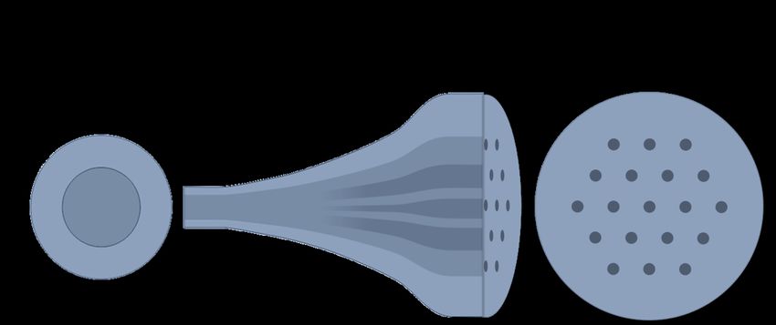
values which are optimised for the problem at hand. A review of the variety of hyperparameters
and an in-depth explanation of NNs can be found in Ref. 28, or a shorter review can be found in
Ref. 29.
    In Sec. 2 we describe the training of NN models based on simulated data created in RSoft’s
BeamPROP. In Sec. 3 we use the same approach to train NN models on optical testbed data taken
using an existing PL in both monochromatic and polychromatic light. We then describe the perfor-
mance of these trained models in Sec. 4.1 before demonstrating two experiments performed with
these models in Sec. 4.2.

2 Creating a neural network model using simulated data
In order to simulate the effects of wavefronts distorted by astronomical seeing passing through a
PL or to identify wavefronts which maximise or minimise the output of a single-mode fibre, we
require a data set with which to train the NN model. In this work we explore training these NN
models on simulated data and on lab measurements of an existing PL, which are compared in
Sec. 4.1. Regardless of the nature of the data used, more accurate NN models can be trained if
larger data sets are available.
    When modelling a theoretical lantern, training data is first produced using a conventional beam
propagation algorithm. Note that the NNs approximate the outcomes of the beam propagation
algorithm, rather than explicitly solving Maxwell’s equations. Thus, the NNs do not replace tra-
ditional beam propagation algorithms, which are required to create a training set which captures
the physics at play in this system. The creation of this training data set takes some time, but once
produced the resulting NN model can be used to rapidly calculate the transmission of any arbitrary
wavefront through the PL. The time taken to create this training data is explored at the end of this
section.
    The simulated data used in this work was generated through the BeamPROP module of RSoft, a
three dimensional optical modelling software that numerically propagates electromagnetic waves
through media of almost arbitrary shape and properties. This ability to handle micro-patterned
structures was exploited to simulate the functioning of a three dimensional PL. We modelled a
19-output multicore fibre lantern with physical properties summarised in Table 1. Propagation
in BeamPROP for a 3D PL with a sufficiently large volume and fine grid size requires about 60
minutes per simulation on four cores of an AMD Threadripper 2990WX.
    The incident light field was assumed to have uniform intensity in the pupil plane, with a ran-
domly varying phase term formed by the superposition of Zernike polynomials in Noll order.30
The strength of each individual Zernike term is governed by a coefficient specifying the root mean
squared (RMS) wavefront error (WFE) contributed by that term. Data sets were created in which
these coefficients were drawn from one of three ranges: ±0.85 radians (±0.2 µm), ±2.1 radians
(±0.5 µm) and ±4.1 radians (±1 µm). With one of the ranges selected, coefficients were drawn

                                                 4
Table 1 The physical properties of the PL, modelled in RSoft, used in this project.
Property Value
Single-mode waveguides 19
Waveguide packing Centred hexagonal
Waveguide length 40 000 µm
Waveguide taper Linear
Waveguide final width, height 6.5 µm
Waveguide refractive index 1.447
Cladding refractive index 1.026
Background refractive index 1
independently and uniformly from within the bounds of the range. Larger ranges, such as ±2.1 ra-
dians and ±4.1 radians we used to ascertain the model’s performance on wavefronts with a larger
RMS WFE. This uniform sampling is likely not optimal in terms of sample efficiency; however, we
chose this method to avoid biasing our data. Poppy31 was used to generate wavefronts described by
these Zernike polynomials. Once created these wavefronts were focused, by Poppy, as if through
an ideal lens and into point spread functions (PSFs). These PSFs were then passed to RSoft to be
injected into the simulated PL. The intensities of the single-mode waveguides were then extracted
from RSoft, and recorded.
The set of Zernike polynomial coefficients used to construct the wavefront and their corre-
sponding set of waveguide intensities formed one training example. Thousands (see Table 3) of
these examples are combined to create the training, validation and testing sets. Since the model
has seen the training data (during training) we assess the model’s performance on the previously
unseen validation set to tune the hyperparameters. As hyperparameters are tuned to optimised per-
formance on the validation set, we can inadvertently bias the model’s performance on this set. For
this reason, the unseen testing set is used to provide the final metrics. In order to ensure the testing
set was large enough to provide accurate metrics each simulated data set has a testing set of 1 000
examples.
We can exploit a symmetry in the PL to augment our training set, i.e. increase the size of the
set without additional computational power. The PL used in this data set has its single-mode fibre
waveguides arrayed in a centred hexagonal lattice which has six-fold rotational symmetry along
each interval of π3 . By rotating our input PSF by π3 radians the pattern observed in the output
waveguides will also rotate by the same amount in an ideal PL. Due to manufacturing defects this
does not currently work on real-world PLs. In order to rotate the PSF, the Zernike polynomials are
5rotated by adjusting the weight given to each polynomial based on Eq. (1) of Ref. 32:
~c
c~0 = T~ (1)
1
m0 = 0
T~nmn0 m0 = δnn0 δ|m||m0 | cos(m0 φ) m0 = m (2)
sin(m0 φ)
m0 = −m
Where c~0 is the vector of Zernike coefficients in the rotated frame, ~c is the vector of Zernike co-
efficients in the original frame and the elements of T~ are defined in Eq. (2). In Eq. (2), φ is the
angle by which c~0 will be rotated, n and n0 are the radial degree of each Zernike polynomial in their
respective frames and m and m0 are the azimuthal frequency of each Zernike polynomial in their
respective frames.
RSoft increments the propagating wavefront through the PL with a user-set interval: the grid
size parameter. There is a balance to be struck with this grid size parameter between fidelity and
speed, as a finer grid size will produce more accurate simulations at the cost of a longer compute
run. This trade space is explored in Table 2, which illustrates the strong computational penalty
imposed by finely sampled spatial grids. The utility of the lower-fidelity simulations is examined
later in this work.
Table 2 Comparison of mean simulation rate for varying RSoft grid sizes. These simulations were run on 4 CPU cores
(on an AMD Threadripper 2990WX) with 16 simulations running in parallel.
X/Y Grid Size Z Grid Size Number of Simulations Mean Minutes
(µm) (µm) in Test Run per Simulation
0.25 2 1 000 51.2
0.5 2 4 000 13.0
1 2 16 000 3.84
3 Creating a model using photonic lantern data from an optical laboratory testbed
Two sets of data were taken in the laboratory using monochromatic and polychromatic illumina-
tion. The monochromatic configuration employed a 685 nm laser with a measured bandwidth of
1.2 nm, collimated to create a plane wave. The beam was then shaped to deliver the required di-
verse population of input wavefronts using a spatial-light modulator. Each pattern was determined
by drawing a set of Zernike polynomial coefficients from a uniform distribution, each yielding a
value between approximately -0.4 and 0.4 radians RMS WFE. The monochromatic data set used
only the first 10 Zernike polynomials, resulting in a mean RMS WFE of 0.744 radians.
6The polychromatic data set employed the same setup, replacing the laser with a broadband
halogen light source. Furthermore, here the first 20 Zernike polynomials in OSA33 order (corre-
sponding to the first 21 Zernike polynomials in Noll order, excluding the 20th) were employed
yielding a mean RMS WFE of 0.950 radians.
The wavefront was then injected into the multimode region of the PL with a microscope objec-
tive. The PL had a visible wavelength multicore fibre with a diameter of 22 µm and a numerical
aperture of 0.145. The multimode region transitions to 19 single-mode cores each with a diameter
of 3.7 µm, a numerical aperture of 0.14 and a core-to-core separation of 35 µm. The outputs of
the single-mode cores were then imaged by a camera with an f = 200 mm doublet lens. Images
collected with this arrangement were accumulated over thousands of input wavefronts to create a
data set, as summarised in Sec. 4.1. The process is extremely rapid: the rate at which data can be
produced is limited only by the frame rate of the camera and software latency (
1 second per
wavefront). Note that this approach treats the entire experimental set-up as one system which will
be modelled by a NN. As such we do not need to model every single lens, but will require that we
re-characterise the system if the PL is moved to a different set-up.
For the polychromatic data, the multicore output was collimated and spectrally dispersed be-
fore imaging onto the camera, with the resulting spectra yielding 31 wavelength channels spaced
between 655.8–751.5 nm for each core.
The monochromatic lab data set had a testing set containing 1 163 examples. The broadband
lab data set had a testing set size of 31 000 examples comprised of Zernike coefficient combinations
which the network had not seen.
4 Results and Discussion
4.1 Model Performance
We trained densely connected feed-forward NNs using Keras34 with an Adam35 optimiser. We
used mean squared error (MSE) as our loss function, Leaky ReLU as our activation function and
batch normalisation36 was used between hidden layers.
We sought to keep the statistical variation in the validation and testing sets as close to a real-
world distribution as possible, so that recorded metrics were directly comparable to realistic appli-
cations. To this end, when using simulated data only the highest fidelity data were included in the
validation and testing sets and no augmentation was applied. The lower fidelity data (generated
with grid sizes > 0.25 µm) was assigned entirely to the training set and this was the only set on
which data augmentation was applied.
Hyperparameters were iteratively tuned to optimise the loss function on each data set. The
difference in MSE between an untuned NN model and one which had been tuned (i.e. hyperpa-
rameters adjusted from some initial value) tended to be around a factor of 2. Ultimately, densely
connected feed-forward networks with hidden layers of constant sizes were found to perform best.
7A list of these hyperparameters and the MSE of each model is presented in Table 3 for the NN
models trained on simulated data sets and Table 4 for NN models trained on the lab data sets.
These tables show that increased RMS WFE and the number of Zernike polynomials requires
more complex models (increased layers) and also results in larger MSE. Plots depicting some of
these models can be seen in Fig. 2.
With RMS WFE greater than 1 radian the output intensities are not a linear function of input
phase.2 The low MSEs throughout demonstrate that not only is this approach capable of emulating
simulated PLs but that the approach also produces extremely accurate results on real-world PLs
and also that the models are capable of accurately predicting even when the RMS WFE is very
large. Figure 3 depicts the difference between a low MSE and an (intentionally) high MSE.
Table 3 Summary of the NN models which best emulated a simulated PL given restrictions on the number and
magnitude of the Zernike polynomial coefficients. Nz is the number of Zernike polynomials which describe the input
wavefront, Reg. is the method of regularisation used and p is the regularisation hyperparameter. The outputs of the
model were normalised such that, on average, sets of intensities from the data set summed to 1. The number of training
examples in brackets is the number of training examples before six-fold augmentation through rotation. Note that these
bracketed numbers are largely comprised of the data with a coarse grid size.
Mean Model Hidden
RMS WFE MSE Layer Training
(radians) Nz (norm. units) Layers Size Reg. p Examples
−5 −7
1.16 7 2.12×10 3 5 000 L2 1.58×10 1 672
−4 −7
1.52 11 2.26×10 4 5 000 L2 1.58×10 1 672
−4 −6
1.86 16 7.00×10 4 2 000 L2 3.98×10 1 900
2.04 19 7.91×10⁻⁴ 17 2 000 None - 6 031
−4
3.15 8 1.22×10 13 2 000 Dropout 0.2 93 528 (15 588)
3.77 11 4.38×10⁻⁴ 9 2 000 Dropout 0.2 291 714 (48 619)
6.28 8 8.42×10⁻⁴ 15 2 000 Dropout 0.2 194 334 (32 389)
A single high-resolution propagation in BeamPROP, using a single quad-core CPU takes around
60 minutes. By using multiple cores per propagation, running propagations in parallel, using a
coarser grid size and augmenting the data through rotations we are able to reduce the time required
to create these training examples. Using these techniques to accelerate data generation, 250 000
training examples can be generated in a week (compared with almost 2 years if no augmentation or
higher-fidelity data is used). Imperfections in the optical testbed removed the symmetries required
for data augmentation. However, lab data can be taken much more quickly than simulated data and
so augmentation is not required in this case.
For the polychromatic data set we used an architecture which included the wavelength as an
input to the model, as shown in Fig. 4. This architecture has the added advantage that the network is
8Table 4 Summary of the NN models which best emulated a physical, pre-existing PL given restrictions on the number
and magnitude of the Zernike polynomial coefficients. The 20-Zernike model was trained and assessed on broadband
data, it predicts outputs based on the first 20-Zernike polynomials in ANSI order and the wavelength of light specified.
Each Zernike polynomial coefficient was selected from a uniform distribution, as specified in the table. Nz is the
number of Zernike polynomials which describe the input wavefront, Reg. is the method of regularisation used and p is
the regularisation hyperparameter. The outputs of the model were normalised such that, on average, sets of intensities
from the data set summed to 1. These data were not augmented through rotation.
Model Hidden
Mean RMS MSE Layer Training
Nz WFE (radians) (norm. units) Layers Size Reg. p Examples
10 0.744 2.97×10⁻⁶ 2 5 000 L2 1.58×10⁻⁷ 57 570
20* 0.950 1.90×10⁻⁵ 8 2 000 Dropout 0.2 1 147 000
able to learn how the PL outputs vary with wavelength, making the network capable of generalising
to unseen wavelengths.
As discussed in Sec. 3, this NN model was trained on data generated by 31 discrete wave-
lengths ranging from 655.8–751.5 nm. To demonstrate that the model accurately predicts unseen
wavelengths in this range, a new NN model was trained on wavelengths from 655.8–697.2 nm and
703.5–751.5 nm and tested on 700.3 nm wavelength data. This NN model, which had identical
hyperparameters to the model described in Table 4, achieved a MSE of 1.97×10⁻⁵ —practically
identical to the predictions made by the full NN model.
4.2 Model Experiments
We demonstrate two possible use-cases of the NN models created in Sec. 4.1. Firstly, we show its
performance in response to simulated astronomical seeing (or other sets of arbitrary WF error) and
secondly it is employed to design optimal injection WFs for specific output-patterns using global
optimisation. In this second case, we chose to formulate designs for two potentially valuable
photonic processes: PL funnels and PL nullers. The advantage of these neural-network models
over traditional beam propagation algorithms lie in their speed and low hardware requirements.
Propagating light through a 3D PL to establish its outputs at a suitably fine grid-size with RSoft’s
BeamPROP takes ∼60 minutes. In contrast, the NN models described in Sec. 4.1 are 5 orders of
magnitude faster. We performed 100 000 tests and found the mean time to propagate through the
NN model was around 0.03 seconds per wavefront propagation when run on a consumer-grade
GPU card (here an Nvidia RTX 2080TI).
4.2.1 Response to Seeing
In the design and evaluation of astronomical systems utilising PLs, it is important to have an end-
to-end model of the system. However, modelling the response of such a system to realistic seeing
9Predicted waveguide output intensity (norm. units)
0.3 7-Zernike Model with 1.16 rad. RMS WFE 0.3 8-Zernike Model with 3.15 rad. RMS WFE
Predicted waveguide output intensity (norm. units)
0.2 0.2
0.1 0.1
0.00.0 0.1 0.2 0.3 0.00.0 0.1 0.2 0.3
True waveguide output intensity (norm. units) True waveguide output intensity (norm. units)
0.3 10-Zernike Model with 0.744 rad. RMS WFE 0.3 20-Zernike Model with 0.95 rad. RMS WFE
Predicted waveguide output intensity (norm. units)
Predicted waveguide output intensity (norm. units)
0.2 0.2
0.1 0.1
0.00.0 0.1 0.2 0.3 0.00.0 0.1 0.2 0.3
True waveguide output intensity (norm. units) True waveguide output intensity (norm. units)
Fig 2 Correlation plot of a random selection of examples from each NN model’s testing set. The top row of plots are
from the best performing models trained on simulated data (Table 3). The bottom row are from models trained on
laboratory measurements of an existing PL (Table 4), i.e. the bottom-left plot is from the monochromatic model and
the bottom-right plot is from the polychromatic model. The black dashed line denotes perfect predictions. The outputs
of the model were normalised such that, on average, sets of intensities from the data set summed to 1.
has been impractical, with an hour per timestep needed when using beam propagation algorithms.
Instead, unrealistic approximations were used—such as flux being evenly distributed between all
outputs regardless of WFE.37 Using the NN models described here, this can be done in near real-
time. Fig. 5 depicts a conceptual scheme where a lantern is deployed to measure these effects.
As illustrated, the seeing results in distorted wavefronts arriving at the telescopes, which then
propagate through to a focus at the input of a PL. Note that when data comes from a real PL, such
10Predicted waveguide output intensity (norm. units)
0.3 Well trained model, MSE = 1.22 × 10 4
0.3 Poorly trained model, MSE = 1.11 × 10 3
Predicted waveguide output intensity (norm. units)
0.2 0.2
0.1 0.1
0.00.0 0.1 0.2 0.3 0.00.0 0.1 0.2 0.3
True waveguide output intensity (norm. units) True waveguide output intensity (norm. units)
Fig 3 Correlation plot showing the difference between a model with low MSE (the left panel) and a model which was
intentionally trained poorly to have a high MSE (the right panel). The poorly trained model is under-regularised and
has overfit the training data.
W1
Z1
W2
Z2
W3
Z3
...
...
...
W17
Zn
W18
W19
Fig 4 Schematics showing the network structure for the polychromatic data. In this figure Zn is the nth Zernike
polynomial and Wn is output of the nth waveguide. In this structure the wavelength is included as an input in addition
to the Zernike polynomial coefficients.
as one in-situ at an adaptive optics (AO) facility, the entire system from deformable mirror (DM)
to single-mode outputs can be modelled—not only the PL.
In order to simulate aberrated wavefronts distorted by seeing which are then passed into a PL,
we used HCIPy38 to generate realistic seeing phase screens, and then OpticsPy39 to decompose the
wavefronts over the Zernike polynomials (as the NN models were trained on this basis). Thirty
seconds of numerically-generated seeing data, sampled at 40 ms time-steps, was fed into the best-
performing NN model on the 8 Zernike data set. The results, presented as a multi-frame “video”,
can be seen in Fig. 6. A plot illustrating the intensities of selected waveguides—numbered in
11Fig 5 Diagram showing starlight wavefronts perturbed by astronomical seeing and subsequently passed into a PL,
resulting in varying outputs. The dashed blue box is the section of the system emulated by the NN models trained in
this work.
Fig. 7—as a function of time can be seen in Fig. 8 or as a waterfall plot in Fig. 9. With the
polychromatic model, trained on a physical PL, we are also able to see the relationship between
wavelength and mode excitement as seeing is passed into the lantern, as shown in Fig. 10.
Passing each frame of the video to a traditional beam propagation algorithm would have taken
over a month; by using the NN model it took around 30 seconds. The models are by no means
limited to 30 seconds of input; they can compute the PL outputs for as many wavefronts as are
provided for ∼ 0.03 s per wavefront.
4.2.2 Funnels and Nullers
When attempting to inject light from an AO-corrected telescope into a fiber or PL, the usual ap-
proach is to maximise the Strehl ratio of the beam (as is usual in AO operations) in order to max-
imise coupling.19, 20 Sometimes apodiziation, such as phase-induced amplitude apodization,20, 40, 41
is used to further improve coupling. However, other potential applications exist wherein a specific
distribution of intensities in the output waveguides from a PL is desired. To achieve this (especially
in the case of a real, manufactured PL), an incident wavefront must be identified which optimally
produces the desired output intensities. This wavefront becomes the new zero-point of the AO
system (rather than aiming for the flattest possible wavefront), and so is restricted to the space
of wavefronts that can be produced by the DM. This is defined by the actuator number, spacing
and maximum stroke of the DM, and the given pupil amplitude distribution. Determining this
wavefront thus requires a global optimisation over this space, with some potentially complicated
or degenerate merit function.
One such application is a so-called “PL funnel”. This is a system that translates some low
Strehl incident optical state and injects it, with high efficiency, into just one (or a small number
12Fig 6 A ‘film-strip’ style representation depicting a segment of video showing neural-network simulation results,
wherein 30 seconds of seeing is propagating through a PL. The left-hand panel shows the turbulent phase screen
which was generated for a windspeed of 10 m/s, the middle panel shows the PSF of the system and the right-hand
panel shows a depiction of the output illumination of the PL. The seeing was generated with a Fried parameter of 0.7 m
for a telescope with a diameter of 8.2 m. The intensity was normalised such that the intensity across all waveguides
for a flat wavefront summed to 1. (Video 1, MP4, 11.9 MB)
of) single-mode waveguides emerging from a PL—rather than distributing it between all outputs.
One could alternatively aim to just directly inject the light into one single-mode fibre, but this has
proved extremely challenging due to the high-degree of wavefront correction required (hampered
by non-common path errors between fibre and wavefront sensor) and mismatch of telescope pupil
1316 15 14
17 5 4 13
18 6 0 3 12
7 1 2 11
8 9 10
Fig 7 Diagram showing the numbering system adopted of the single-mode waveguides at output.
Selected Intensity vs Time, Fried Parameter = 0.7m
0.25
Null 1
Null 2
0.20 Null 3
Non-Null 1
Non-Null 2
Normalised Intensity
Non-Null 3
0.15
0.10
0.05
0.00
0 1 2 3 4 5
Time (s)
Fig 8 A plot of neural-network simulation results showing the intensity of selected waveguides versus time, as seeing
is passed into the PL. Waveguide 0 is the central waveguide, waveguide 1 is a waveguide in the inner-ring, waveguide
8 is a corner-waveguide in the outer ring and waveguide 9 is an edge-waveguide in the outer ring. This seeing was
generated with a a windspeed of 10 m/s and a Fried parameter of 0.7 m for a telescope with diameter of 8.2 m. The
intensity was normalised such that the intensity across all waveguides for a flat wavefront summed to 1. (Video 1,
MP4, 11.9 MB)
amplitude (and resulting PSF) with the fibre’s mode field. By using a PL the target wavefront can
be optimised to maximise injection, and light leaking into the ‘dark’ outputs could be used as a
wavefront sensor to maintain this target wavefront without non-common path errors2 . It also allows
light to be injected into a small number of waveguides, capturing light which would be lost (due to
poor AO correction) if a single single-mode fibre was used. Once light is in a single-mode fibre,
the size of a spectrograph no longer scales with the number spatial modes in a telescope, allowing
small, compact spectrographs.16–18, 42–44 These small spectrographs are more easily stabilised and
140
2 0.25
4
0.20
Normalised Intensity
Waveguide Number
6
8 0.15
10
12 0.10
14
0.05
16
18 0.00
0 2 4 6 8 10 12 14 16 18 20 22 24 26 28 30
Time (s)
Fig 9 A waterfall-style plot of neural-network simulation results, showing the shifting waveguide intensities in re-
sponse to seeing. Seeing was generated assuming a windspeed of 10 m/s and a Fried parameter of 0.7 m for a
telescope with diameter of 8.2 m. The intensity was normalised such that the intensity across all waveguides for a flat
wavefront summed to 1. (Video 1, MP4, 11.9 MB)
Fig 10 A waterfall-style plot of polychromatic neural-network simulation results, showing the intensity as a function of
wavelength as seeing is passed through the NN model, for selected waveguides. Waveguide 0 is the central waveguide,
waveguide 1 is a waveguide in the inner-ring, waveguide 8 is an edge-waveguide in the outer ring and waveguide 9
is a corner-waveguide in the outer ring. In sections where the seeing is outside the range of the model (i.e. one of
the Zernike coefficients is greater than ∼ 0.35 radians) predictions may be less reliable. The intensity was normalised
such that the intensity across all waveguides for a flat wavefront summed to 1.
15cheaper to fabricate, enabling a greater number of objects to be observed concurrently if several
are placed in a telescope.
A PL nuller is the converse of an PL funnel. Instead of attempting to identify a wavefront
which maximises the coupling into a single waveguide of a PL we seek to minimise light into that
waveguide.45 A nulling interferometer (hereafter nuller) is particularly useful when attempting
to observe faint objects (such as an exoplanet) which are in close proximity to a bright source
(typically the host star).46 Interference is created between two telescopes (or regions of a telescope
pupil) to cancel out the unwanted bright source, such as a central star, preserving the much fainter
signal from nearby objects (e.g. circumstellar disk or planet). This has previously been done using
traditional bulk optics47, 48 and also by photonic techniques in testbed instruments such as GLINT45
and PFN.49, 50 As explored here, by carefully choosing an incident wavefront a PL could potentially
serve a similar function.
Identifying the precise wavefronts that result in funnels or nullers can be accomplished with
a global optimsation algorithm. For this project, SciPy’s51 basinhopping optimisation func-
tion was employed which implements the basin-hopping algorithm described by Wales & Doye.52
These optimisations explored the space of Zernike polynomial coefficients which, when passed
through the NN model, achieved waveguide intensities that minimised our objective function (see
Equation 3 below).
Over the course of the optimisation process described here, around 65 000 calls to the model
were made. This would have taken of order 5 and a half years if the wavefronts had been passed
through a traditional beam propagation algorithm. Using the models constructed for this work
(which take around 0.03 seconds to map an incident wavefront into a pattern of single-mode output
intensities) the entire global optimisation described can run to completion in under an hour.
In this work, the most severe of the constraints are (1) the restriction on the amplitude (constant
across the pupil, apart from zeros at regions shadowed by telescope structures), and (2) the limited
set of spatial frequencies that can be produced by the DM. Here, the set of functions chosen to
represent the phase is the Zernike basis. The goal is to maximise (or minimise) the light through a
number of waveguides while remaining agnostic to which specific waveguides contribute.
If no such constraints existed, and there was no degeneracy in the desired output intensity
pattern (e.g. all flux in one specific waveguide), then it is trivial to obtain an ideal solution for a
theoretical PL. Employing traditional beam propagation software such as RSoft, propagating light
from the single desired waveguide in the reverse fashion through the lantern yields the electric
field at the multimode region before the adiabatic taper. Conjugating this electric field results in a
wavefront which, if passed through the PL, would maximally excite that single waveguide. This
method yielded the solution shown in Fig. 11, which, it was confirmed, resulted in the expected
perfect funnel operation under forward propagation back through the lantern. Unlike situations
where two or more waveguides are illuminated, in the case of a single illuminated waveguide
16the solution is uniquely defined. Unfortunately, as the wavefront is described by strong, high-
frequency variations in both amplitude and phase, it violates the terms of our constraints listed
above. Therefore the task becomes an optimisation problem.
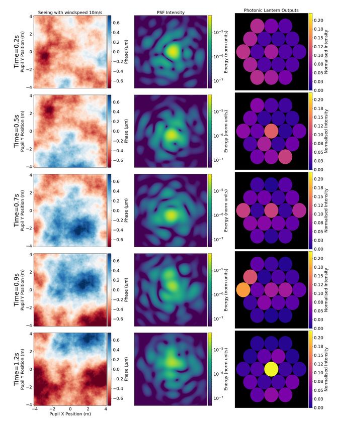
Fig 11 Depictions of the phase and amplitude required to create a perfect PL funnel into the central waveguide, i.e. a
wavefront which results in 100% of light passing through the central waveguide. Note the non-uniform amplitude in
the far field (equivalent to the telescope pupil) and very high spatial frequencies—which prevents the formulation of
this wavefront by a DM.
One example is to optimise for the largest possible fraction of the light being contained in any
one single waveguide, with the remaining light shared in any fashion among the others. This al-
lows the optimiser to choose not only the optimum achievable wavefront, but also the target output
waveguide which allows the best results. A second possibility is to identify an input which max-
imises the total light channeled into some small number of waveguides; for example, attempting
to find a pattern yielding two or three waveguides containing almost all the flux.
Unlike a perfect PL funnel, the solution for a PL nuller is not unique. Therefore solutions
which completely extinguish the output of a single waveguide are relatively plentiful. Addition-
ally, we may choose to add further (scientifically valuable) constraints; specifically, nulling mul-
tiple waveguides simultaneously. Indeed, the optimisation can find such solutions allowing us to
further explore the trade-off between the number of near-null outputs and the degree of extinction
(quantified by, for example, the cumulative light into the nulled waveguides).
4.2.3 Identified funnel and nuller solutions
As our lantern contains 19 waveguides at output and we are restricted to modulating pupil-plane
phase, there are 19 solutions which maximise light into a single waveguide. These were found
using the basin-hopping algorithm, with the objective function defined to minimise the flux in a
17given waveguide. Figure 12 shows some of the outcomes produced by these optimisations using
the 8-Zernike 3.15 radian RMS WFE model.
These results show that the best funnel for a single waveguide attempts to maximise light in the
central waveguide, achieving 34% of total intensity. Solutions for the best funnel for the 1st, 2nd,
3rd, 4th, 5th, and 6th waveguides—numbered in Fig. 7—are all hexagonal rotations of the same
underlying pattern, as expected. Similarly the same degeneracy exists in solutions among the 7th,
9th, 11th, 13th, 15th and 17th and the 8th, 10th, 12th, 14th, 16th and 18th waveguides due to the
six-fold rotational symmetry in the system as was discussed in the data augmentation portion of
Sec. 2.
Pupil Phase PSF Intensity Mock Output Waveguides
0.3
Energy (norm. units)
Normalised Intensity
2 10 5
Radians
0.2
Maximising light into 0 10 6
waveguide 0; 34%
of light was funnelled. 0.1
2
10 7
Pupil Phase PSF Intensity Mock Output Waveguides 0.0
0.3
Energy (norm. units)
Normalised Intensity
2 10 5
Radians
0.2
Maximising light into 0 10 6
waveguide 1; 32%
of light was funnelled. 0.1
2
10 7
Pupil Phase PSF Intensity Mock Output Waveguides 0.0
0.3
Energy (norm. units)
Normalised Intensity
2 10 5
Radians
0.2
Maximising light into 0 10 6
waveguide 15; 30%
of light was funnelled. 0.1
2
10 7
Pupil Phase PSF Intensity Mock Output Waveguides 0.0
0.3
Energy (norm. units)
2 10 5 Normalised Intensity
Radians
0.2
Maximising light into 3 0 10 6
waveguides; 67% of light
was funnelled. 0.1
2
10 7
0.0
Fig 12 Depiction of the results of the basin-hopping algorithm utilising the 8-Zernike 3.15 radian RMS WFE model,
tasked with seeking to maximise the light intensity through each individual waveguide. Note that since the model only
supports 8 Zernike polynomials the maximum spatial frequency is limited by this constraint rather than the spatial-
light modulator; using a model with a greater number of supported Zernike polynomials would expand this limit. The
left image in each row is a representation of the phase of the wavefront at the pupil, i.e. as it arrives at the optical
system, the central image is the PSF which is injected into the PL, and the final image is an end-on depiction of the PL
showing the intensity of each waveguide. The intensity was normalised such that the intensity across all waveguides
for a flat wavefront summed to 1.
A similar technique can be used to null a set of outputs. Figure 13 shows the solutions found
by the basin-hopping algorithm set to extinguish the exiting light through the specified number
18of waveguides—note that we don’t specify which waveguides—while also maximising the total
amount of light which propagates through the lantern. This was done by combining these two
goals into a single objective function as is shown in Eq. (3) below, which was then set to be
minimised by the gradient descent algorithm:
18
X n
X
f (x, n) = 1 − xi + xi (3)
i=0 i=0
Where x is a list of waveguide intensities sorted in ascending order, xi is the ith lowest intensity of
the waveguides and n is the number of waveguides to be nulled. Note that there are 19 waveguides
in the PL used in this work and so the sum from x0 to x18 is a sum over every waveguide.
These results show that a wavefront solution for a PL nuller capable of effectively extinguishing
a single waveguide, or even a handful of waveguides, can be recovered. If we wish to extinguish
larger numbers of waveguides, then we must accept solutions which let an increasing fraction of
light through the nulled waveguides. As shown in Fig. 13, 1–3 nulled waveguides let 0–1% (to 1
significant figure) of light through, attempting nulling on 7 waveguides results in ∼ 5% of light
leakage into those guides, while a 9-waveguide design results in ∼ 8% leakage into the nulled
channels. Numbers stated here are accurate to the nearest percent, since the MSE of this model is
1.22 × 10⁻⁴ radians the RMS error is of order 10−2 .
We can then examine the effect of these solutions when encountering atmospheric seeing (or
residual WFE after AO correction). The seeing was generated as described in Sec. 4.2.1. The
found solution wavefront was effectively set as the new zero-point of the AO system by adding it
to the seeing-induced wavefront, and so the nulled waveguides, assuming good seeing correction,
should be extinguished. A line plot showing the results of this nulling can be seen in Fig. 14. It
shows that as the seeing is better corrected, the PL nuller is better able to null out the specified
waveguides.
5 Future Work
Training a NN model capable of making predictions based on wavefronts described by more
Zernike polynomials would simply require more data. While the techniques outlined in Sec. 2
mitigate the need for data (and make it faster to generate), it is still ultimately a stumbling block
for creating these NN models from beam-propagation simulations. We found that as the size of
the Zernike space increased so too did the number of hidden layers which resulted in the best
performance. Thus, increasing the number of Zernike polynomials or the RMS WFE range will
likely involve training larger NNs. As the number of hidden layers increases it is possible that a
ResNet-style structure53 will prove optimal. We found that larger models were best regularised
with Dropout.
19Pupil Phase PSF Intensity Mock Output Waveguides
0.3
Energy (norm. units)
Normalised Intensity
2 10 5
Radians
0.2
0 10 6
Darkening 1 waveguides;
0% of light let through. 0.1
2
10 7
0.0
Pupil Phase PSF Intensity Mock Output Waveguides
0.3
Energy (norm. units)
Normalised Intensity
2 10 5
Radians
0.2
0 10 6
Darkening 2 waveguides;
1% of light let through. 0.1
2
10 7
0.0
Pupil Phase PSF Intensity Mock Output Waveguides
0.3
Energy (norm. units)
Normalised Intensity
2 10 5
Radians
0.2
0 10 6
Darkening 3 waveguides;
1% of light let through. 0.1
2
10 7
0.0
Pupil Phase PSF Intensity Mock Output Waveguides
0.3
Energy (norm. units)
Normalised Intensity
2 10 5
Radians
0.2
0 10 6
Darkening 7 waveguides;
5% of light let through. 0.1
2
10 7
0.0
Pupil Phase PSF Intensity Mock Output Waveguides
0.3
Energy (norm. units)
Normalised Intensity
2 10 5
Radians
0.2
0 10 6
Darkening 8 waveguides;
7% of light let through. 0.1
2
10 7
0.0
Pupil Phase PSF Intensity Mock Output Waveguides
0.3
Energy (norm. units)
Normalised Intensity
2 10 5
Radians
0.2
0 10 6
Darkening 9 waveguides;
8% of light let through. 0.1
2
10 7
0.0
Fig 13 Depiction of the results (accurate to the nearest percent) of the basin-hopping algorithm utilising the best
performing 8-Zernike 3.15 radian RMS WFE model, tasked to minimise the light through some number of waveguides.
The crosses indicate the waveguides which were chosen by the algorithm to darken. The robustness of these nulls to
an incorrect DM position is explored in Fig. 14. The left image in each row is a representation of the phase of the
wavefront at the pupil, i.e. as it arrives at the optical system, the central image is the PSF which is injected into
the PL in each case and the final image is an end-on depiction of the PL showing the intensity of each waveguide
after the lantern has been injected with this wavefront. The intensity was normalised such that the intensity across all
waveguides for a flat wavefront summed to 1.
We chose to use the Zernike polynomials to describe our input wavefront however this is not the
only choice; future NN models could use a actuator basis of the DM. While this greatly increases
the dimensionality of the input space it does remove some of the restrictions imposed on the space
by the use of a finite number of Zernike polynomials. There is promising research suggesting that
20Selected Intensity vs Time, Fried Parameter = 0.7m Selected Intensity vs Time, Fried Parameter = 2.0m
0.25 0.25
Null 1 Null 1
Null 2 Null 2
Null 3 Null 3
0.20 Non-Null 1 0.20 Non-Null 1
Non-Null 2 Non-Null 2
Non-Null 3 Non-Null 3
Normalised Intensity
Normalised Intensity
0.15 0.15
0.10 0.10
0.05 0.05
0.00 0.00
0 1 2 3 4 5 0 1 2 3 4 5
Time (s) Time (s)
Selected Intensity vs Time, Fried Parameter = 7.0m
0.25
Null 1
Null 2
Null 3
0.20 Non-Null 1
Non-Null 2
Non-Null 3
Normalised Intensity
0.15
0.10
0.05
0.00
0 1 2 3 4 5
Time (s)
Fig 14 Diagram showing the effect of applying our 3-nuller solution to seeing. The seeing in the top-left plot was
created with a Fried parameter of 0.7 m. The seeing in the top-right plot was created with a Fried parameter of 2 m.
The seeing in the bottom plot was created with a Fried parameter of 7 m. In all cases the data was created for telescope
with an 8.2 m diameter experiencing a wind speed of 10 m/s. The intensity was normalised such that the intensity
across all waveguides for a flat wavefront summed to 1.
a CNN54 would be best suited to this task due to its innate spatial reasoning.
While we demonstrated NN model performance on a single physical PL (see Table 4) there is
no reason these models shouldn’t work on any PLs if training data is provided.
With enough training data it should be possible to characterise propagation through a PL with
a physical structure unseen in the training set. Similar to the polychromatic network structure
described in Sec. 3, a network could be trained which took as inputs various parameters which
describe the PL’s design. Once trained, such a model could then predict the outputs of PLs with
arbitrary properties. This would allow PLs which vary in waveguide length, waveguide width,
waveguide refractive index or cladding refractive index to be characterised. The volume of data
required for this characterisation is estimated to be 1–2 orders of magnitude greater than that for a
single PL.
216 Conclusion
Photonic lanterns are an exciting technology with a wide variety of applications in astronomy, op-
tics and telecommunications. Successful, widespread deployment for single-mode spectroscopy,
interferometry and other astrophotonic applications will require fast and accurate simulation tools
for design and testing. However, traditional beam propagation algorithms applied to these three
dimensional photonic devices are slow enough (∼ 1 hour per propagation on a single quad-core
CPU) to make them impractical for some uses. We developed neural network models capable of ac-
curately predicting a photonic lantern’s output in 0.03 s, a speed-up of over 5 orders of magnitude.
This technique was used to model existing photonic lanterns—including manufacturing defects—
and was also shown to generalise to polychromatic inputs. Using these models, the response of
each of the photonic lantern’s outputs can be predicted as a function of an arbitrary seeing time-
series, over a range of wavelengths. We also demonstrated two possible applications: modelling
a photonic lantern’s response to seeing and using a global optimiser to identify wavefront shapes
which act as photonic lantern funnels and nullers.
Acknowledgments
We would like to thank the team at Olivier Guyon, Nemanja Jovanovic and Julien Lozi for their
stimulating discussions.
Code, Data, and Materials Availability
We have made all code freely available at:
https://github.com/David-Sweeney/Learning-the-Lantern
Simulated data is freely available in the supplementary material. Data from the optical testbed
may be made available upon personal request.
References
1 S. G. Leon-Saval, T. A. Birks, J. Bland-Hawthorn, et al., “Multimode fiber devices with
single-mode performance,” Opt. Lett. 30, 2545–2547 (2005).
2 B. R. Norris, J. Wei, C. H. Betters, et al., “An all-photonic focal-plane wavefront sensor,”
Nature Communications 11(1), 1–9 (2020).
3 N. Jovanovic, R. J. Harris, and N. Cvetojevic, “Astronomical applications of multi-core fiber
technology,” IEEE Journal of Selected Topics in Quantum Electronics 26(4), 1–9 (2020).
4 M. Diab and S. Minardi, “Modal analysis using photonic lanterns coupled to arrays of waveg-
uides,” Opt. Lett. 44, 1718–1721 (2019).
5 T. Anagnos, R. J. Harris, M. K. Corrigan, et al., “Simulation and optimisation of an as-
trophotonic reformatter,” Monthly Notices of the Royal Astronomical Society 478, 4881–4889
(2018).
226 N. Cvetojevic, N. Jovanovic, S. Gross, et al., “Modal noise in an integrated photonic lantern
fed diffraction-limited spectrograph,” Opt. Express 25, 25546–25565 (2017).
7 J. Montoya, C. Hwang, D. Martz, et al., “Photonic lantern kw-class fiber amplifier,” Opt.
Express 25, 27543–27550 (2017).
8 S. Gross, D. W. Coutts, M. Dubinskiy, et al., “Beam shaping of a broad-area laser diode using
3d integrated optics,” Opt. Lett. 44, 831–834 (2019).
9 I. Ozdur, P. Toliver, A. Agarwal, et al., “Single mode collection efficiency enhancement for
free space systems using photonic lantern,” in Advanced Photonics 2013, Advanced Photon-
ics 2013 , SW3D.5, Optical Society of America (2013).
10 N. K. Fontaine and R. Ryf, “Characterization of mode-dependent loss of laser inscribed pho-
tonic lanterns for space division multiplexing systems,” in 2013 18th OptoElectronics and
Communications Conference held jointly with 2013 International Conference on Photon-
ics in Switching, 2013 18th OptoElectronics and Communications Conference held jointly
with 2013 International Conference on Photonics in Switching , Optical Society of America
(2013).
11 R. R. Thomson, “Ultrafast laser inscription of 3D components for spatial multiplexing,” in
Next-Generation Optical Communication: Components, Sub-Systems, and Systems V, G. Li
and X. Zhou, Eds., 9774, 143 – 148, International Society for Optics and Photonics, SPIE
(2016).
12 R. . Essiambre, R. Ryf, N. K. Fontaine, et al., “Breakthroughs in photonics 2012: Space-
division multiplexing in multimode and multicore fibers for high-capacity optical communi-
cation,” IEEE Photonics Journal 5(2), 0701307–0701307 (2013).
13 S. G. Leon-Saval, N. K. Fontaine, and R. Amezcua-Correa, “Photonic lantern as mode multi-
plexer for multimode optical communications,” Optical Fiber Technology 35, 46–55 (2017).
Next Generation Multiplexing Schemes in Fiber-based Systems.
14 Z. S. Eznaveh, J. C. A. Zacarias, J. E. A. Lopez, et al., “Photonic lantern broadband orbital
angular momentum mode multiplexer,” Opt. Express 26, 30042–30051 (2018).
15 H. K. Chandrasekharan, F. Izdebski, I. Gris-Sánchez, et al., “Multiplexed single-mode
wavelength-to-time mapping of multimode light,” Nature Communications 8(1) (2017).
16 J. Bland-Hawthorn, J. Lawrence, G. Robertson, et al., “PIMMS: photonic integrated mul-
timode microspectrograph,” Ground-based and Airborne Instrumentation for Astronomy III
7735(December 2014), 77350N (2010).
17 C. H. Betters, S. G. Leon-Saval, J. G. Robertson, et al., “Beating the classical limit: A
diffraction-limited spectrograph for an arbitrary input beam,” Opt. Express 21, 26103–26112
(2013).
2318 C. Schwab, S. G. Leon-Saval, C. H. Betters, et al., “Single mode, extreme precision doppler
spectrographs,” Proceedings of the International Astronomical Union 8(S293), 403–406
(2012).
19 N. Jovanovic, C. Schwab, O. Guyon, et al., “Efficient injection from large telescopes into
single-mode fibres: Enabling the era of ultra-precision astronomy,” Astronomy & Astro-
physics 604 (2017).
20 N. Jovanovic, N. Cvetojevic, B. Norris, et al., “Demonstration of an efficient, photonic-based
astronomical spectrograph on an 8-m telescope,” Optics Express 25 (2017).
21 A. Krizhevsky, I. Sutskever, and G. E. Hinton, “ImageNet Classification with Deep Convo-
lutional Neural Networks,” Advances in neural information processing systems , 1097–1105
(2012).
22 D. Silver, A. Huang, C. J. Maddison, et al., “Mastering the game of Go with deep neural
networks and tree search,” Nature 529(7587), 484–489 (2016).
23 D. N. Ganesan, D. Venkatesh, D. M. A. Rama, et al., “Application of Neural Networks in
Diagnosing Cancer Disease using Demographic Data,” International Journal of Computer
Applications 1(26), 81–97 (2010).
24 J. N. Wei, D. Duvenaud, and A. Aspuru-Guzik, “Neural networks for the prediction of organic
chemistry reactions,” ACS Central Science 2(10), 725–732 (2016).
25 S. G. Leon-Saval, A. Argyros, and J. Bland-Hawthorn, “Photonic lanterns,” Nanophotonics
2(5-6), 429–440 (2013).
26 D. E. Rumelhart, G. E. Hinton, and R. J. Williams, “Learning representations by back-
propagating errors,” Nature 323, 533–536 (1986).
27 N. Srivastava, G. Hinton, A. Krizhevsky, et al., “Dropout: A simple way to prevent neu-
ral networks from overfitting,” Journal of Machine Learning Research 15(56), 1929–1958
(2014).
28 F. Emmert-Streib, Z. Yang, H. Feng, et al., “An introductory review of deep learning for
prediction models with big data,” Frontiers in Artificial Intelligence 3, 4 (2020).
29 Y. Lecun, Y. Bengio, and G. Hinton, “Deep learning,” Nature 521, 436–444 (2015).
30 R. J. Noll, “Zernike polynomials and atmospheric turbulence∗,” J. Opt. Soc. Am. 66, 207–211
(1976).
31 M. D. Perrin, R. Soummer, E. M. Elliott, et al., “Simulating point spread functions for the
James Webb Space Telescope with WebbPSF,” in SPIE, M. C. Clampin, G. G. Fazio, H. A.
MacEwen, et al., Eds., 84423D (2012).
32 L. Li, B. Zhang, Y. Xu, et al., “Analytical method for the transformation of Zernike poly-
nomial coefficients for scaled, rotated, and translated pupils,” Applied Optics 57(34), F22
(2018).
24You can also read