BEAT Unintended Bias in Personalized Policies - Eva Ascarza Ayelet Israeli Working Paper 22-010 - Harvard ...
←
→
Page content transcription
If your browser does not render page correctly, please read the page content below
BEAT Unintended Bias in
Personalized Policies
Eva Ascarza
Ayelet Israeli

Working Paper 22-010
BEAT Unintended Bias in
 Personalized Policies
 Eva Ascarza
 Harvard Business School

 Ayelet Israeli
 Harvard Business School

 Working Paper 22-010

Copyright © 2021 by Eva Ascarza and Ayelet Israeli.
Working papers are in draft form. This working paper is distributed for purposes of comment and discussion only. It may
not be reproduced without permission of the copyright holder. Copies of working papers are available from the author.
Funding for this research was provided in part by Harvard Business School.
∗
               BEAT Unintended Bias in Personalized Policies

                                  Eva Ascarza†               Ayelet Israeli‡

                                                August 2021

                                                  Abstract

          An inherent risk of algorithmic personalization is disproportionate targeting of individuals
      from certain groups (or demographic characteristics such as gender or race), even when the
      decision maker does not intend to discriminate based on those “protected” attributes. This
      unintended discrimination is often caused by underlying correlations in the data between pro-
      tected attributes and other observed characteristics used by the algorithm (or machine learning
      (ML) tool) to create predictions and target individuals optimally. Because these correlations
      are hidden in high dimensional data, removing protected attributes from the database does
      not solve the discrimination problem; instead, removing those attributes often exacerbates the
      problem by making it undetectable and, in some cases, even increases the bias generated by the
      algorithm.
          We propose the BEAT (Bias-Eliminating Adapted Trees) framework to address these
      issues. This framework allows decision makers to target individuals based on differences in
      their predicted behavior — hence capturing value from personalization — while ensuring that
      the allocation of resources is balanced with respect to the population. Essentially, the method
      only extracts heterogeneity in the data that is unrelated to those protected attributes. To do
      so, we build on the General Random Forest (GRF) framework (Wager and Athey 2018; Athey
      et al. 2019) and develop a targeting allocation that is “balanced” with respect to protected
      attributes. We validate the BEAT framework using simulations and an online experiment
      with N=3,146 participants. This framework can be applied to any type of allocation decision
      that is based on prediction algorithms, such as medical treatments, hiring decisions, product
      recommendations, or dynamic pricing.

      Keywords: algorithmic bias, personalization, targeting, generalized random forests (GRF),
      fairness, discrimination.
      JEL Classification: C53, C54, C55, M31.

  ∗
     We thank seminar participants at the McCombs School of Business, the 2021 Marketing Science conference, and
the 2021 IMS/HBS Data Science conference for their helpful comments. Hengyu Kuang provided invaluable support,
and Shar Shah and Meng Yang provided excellent research assistance.
   †
     Associate Professor of Marketing at Harvard Business School, eascarza@hbs.edu
   ‡
     Associate Professor of Marketing at Harvard Business School, aisraeli@hbs.edu

                                                       1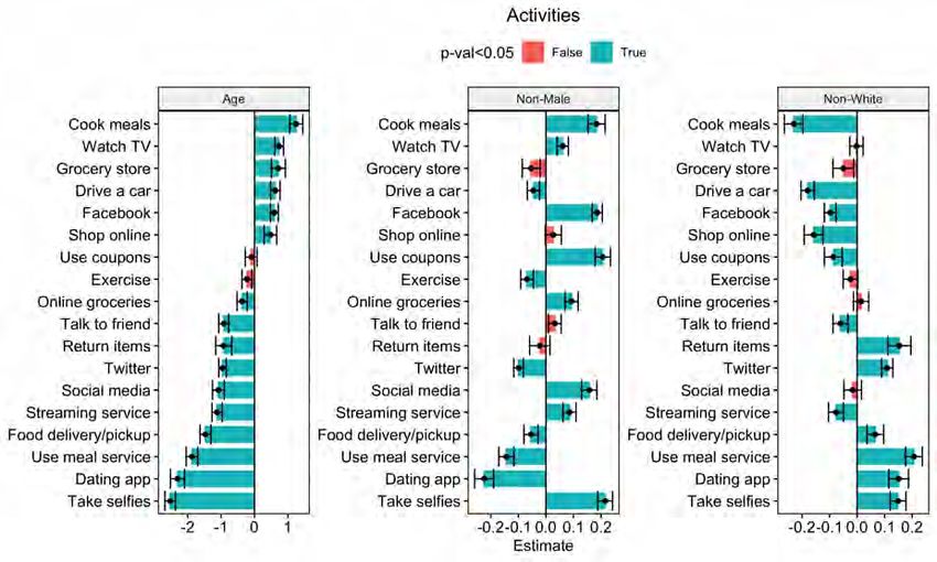
1     Introduction
In the era of algorithmic personalization, resources are often allocated based on individual-level
predictive models. For example, financial institutions allocate loans based on individuals’ expected
risk of default, advertisers display ads based on users’ likelihood to respond to the ad, hospitals
allocate organs to patients based on their chances to survive, and marketers allocate price discounts
based on customers’ propensity to respond to such promotions. The rationale behind these practices
is to leverage differences across individuals, such that a desired outcome can be optimized via
personalized or targeted interventions. For example, a financial institution would reduce risk of
default by approving loans to individuals with the lowest risk of defaulting, advertisers would
increase profits when targeting ads to users who are most likely to respond to those ads, and so
forth.

       There are, however, individual differences that firms may not want to leverage for person-
alization, as they might lead to disproportionate allocation to a specific group. These individual
differences may include gender, race, sexual orientation, or other protected attributes. In fact, sev-
eral countries have instituted laws against discrimination based on protected attributes in certain
domains (e.g., in voting rights, employment, education, and housing). However, discrimination in
other domains is lawful but is often still perceived as unfair or unacceptable (Pope and Sydnor
2011). For example, it is widely accepted that ride-sharing companies set higher prices during peak
hours, but these companies were criticized when their prices were found to be systematically higher
in non-white neighborhoods compared to white areas (Pandey and Caliskan 2021).

      In practice, personalized allocation decisions may lead to algorithmic bias towards a protected
group. Personalized allocation algorithms typically use data as input to a two-stage model: first,
the data are used to predict accurate outcomes based on the observed variables in the data (the
“Inference” stage). Then, these predictions are used to create an optimal targeting policy with a
particular objective function in mind (the “Allocation” stage). The (typically unintended) biases
in the policies might occur because the protected attributes are often correlated with the predicted
outcomes. Thus, using either the protected attributes themselves or variables that are correlated
with those protected attributes in the inference stage may generate a biased allocation policy.1

      Intuitively, a potentially attractive solution to this broad concern of protected attributes-
based discrimination may be to remove the protected attributes from the data and to generate a
personalized allocation policy based on the predictions obtained from models trained using only
the non-protected attributes. However, such an approach would not solve the problem as there
might be other variables that remain in the dataset and that are related to the protected attributes

   1
     Note, algorithmic bias may also occur due to unrepresentative or biased data. This paper focuses on bias that is
created due to underlying correlations in the data.

                                                         2
and therefore will still generate bias. Interestingly, as we show in our empirical section, remov-
ing protected attributes from the data can actually increase the degree of discrimination on the
protected attributes — i.e., a firm that chooses to exclude protected attributes from its database
might create a greater imbalance. This finding is particularly relevant today because companies
are increasingly announcing their plans to stop using protected attributes in fear of engaging in
discrimination practices. In our empirical section we show the conditions under which this finding
applies in practice.

       This biased personalization problem could be in principle solved using constrained optimiza-
tion, focusing on the allocation stage of the algorithm (e.g., Goh et al. 2016; Agarwal et al. 2018).
Using this approach, a constraint is added to the optimization problem such that individuals who
are allocated to receive treatment (the “targeted” group) are not systematically different in their
protected attributes from those who do not receive treatment. Although methods for constrained
optimization problems often work well in low dimensions, they are sensitive to the curse of dimen-
sionality (e.g., if there are multiple protected attributes). Another option would be to focus on
the data that are fed to the algorithm and “de-bias” the data before it is used. That is, transform
the non-protected variables such that they are independent of the protected attributes and use the
resulting data in the two-stage model (e.g., Feldman et al. 2015; Johndrow and Lum 2019). These
models are also sensitive to dimensionality (of protected attributes and of the other variables in
the data), thereby becoming impractical. Further, it is difficult to account for dependencies across
interactions of the different variables (and the outcome variables). Lastly, while these methods
ensure statistical parity, they often harm individual fairness (Castelnovo et al. 2021) because they
transform the value of the non-protected variables based on the protected attribute.2

       Instead, our approach focuses on the inference stage wherein we define a new object of in-
terest — “conditional balanced targetability” (CBT) — that measures the adjusted treatment effect
predictions, conditional on a set of unprotected variables. Essentially, we create a mapping from
unprotected attributes to a continuous targetability score that leads to balanced allocation of re-
sources with respect to the protected attributes. Previous papers that modified the inference stage
(e.g., Kamishima et al. 2012; Woodworth et al. 2017; Zafar et al. 2017; Zhang et al. 2018; Donini
et al. 2020) are limited in their applicability because they typically require additional assumptions
and restrictions and are limited in the type of classifiers they apply to. The benefits of our ap-
proach are noteworthy. First, we leverage computationally-efficient methods for inference that are
easy to implement in practice and also have desirable scalability properties. Second, out-of-sample
predictions for CBT do not require protected attributes as an input. In other words, firms or
institutions seeking allocation decisions that do not discriminate on protected attributes only need
to collect the protected attributes when calibrating the model. Once the model is estimated, future

   2
    Individual fairness ensures that individuals of different protected groups that have the same value of non-protected
attributes are treated equally.

                                                           3
allocation decisions can be based on out-of-sample predictions, which merely require unprotected
attributes.

       In this paper we propose a practical solution where the decision maker can leverage the
value of personalization without the risk of disproportionately targeting individuals based on pro-
tected attributes. The solution, which we name BEAT (Bias-Eliminating Adapted Trees), generates
individual-level predictions that are independent of any pre-selected protected attributes. Our ap-
proach builds on generalized random forests (GRF) (Wager and Athey 2018; Athey et al. 2019),
which are designed to efficiently estimate heterogenous outcomes. Our method preserves most of
the core elements of GRF, including the use of forests as a type of adaptive nearest neighbor esti-
mator, and the use of gradient-based approximations to specify the tree-split point. Importantly,
we depart from GRF in how we select the optimal split for partitioning. Rather than using diver-
gence between children nodes as the primary objective of any the partition, the BEAT algorithm
combines two objectives — heterogeneity in the outcome of interest and homogeneity in the pro-
tected attributes — when choosing the optimal split. Essentially, the BEAT method only identifies
individual differences in the outcome of interest (e.g., response to price) that are homogeneously
distributed in the protected attributes (e.g., race).

      Using a variety of simulated scenarios, we show that our method exhibits promising empirical
performance. Specifically, BEAT reduces the unintended bias while leveraging value of personalized
targeting. Further, BEAT allows the decision maker to quantify the trade-off between performance
and discrimination. We also examine the conditions under which the intuitive approach of removing
protected attributes from the data alleviates or increases the bias. Finally, we apply our solution
to a marketing context in which a firm decides which customers to target with a discount coupon.
Using an online sample of N=3,146 participants, we find strong evidence of correlations between
“protected” and “unprotected” attributes in real data. Moreover, applying personalized targeting
to these data leads to significant bias against a “protected” group (in our case, older population)
due to these underlying correlations. Finally, we demonstrate that the BEAT framework mitigates
the bias, generating a balanced targeting policy that does not discriminate against individuals based
on protected attributes.

       Our contribution fits broadly into the vast literature on fairness and algorithmic bias (e.g.,
Williams et al. 2018; Lambrecht and Tucker 2019; Cowgill 2019; Raghavan et al. 2020; Kleinberg
et al. 2020; Cowgill and Tucker 2020; Pandey and Caliskan 2021). Most of this literature has focused
on uncovering biases and their causes, and on conceptualizing the algorithmic bias problem and
potential solutions for researchers and practitioners. We complement this literature by providing
a practical solution that prevents algorithmic bias that is caused by underlying correlations. Our
work also builds on the growing literature on treatment personalization (e.g., Hahn et al. 2020;
Kennedy 2020; Nie et al. 2021; Simester et al. 2020; Yoganarasimhan et al. 2020; Athey and Wager
2021). This literature has mainly focused on the estimation of heterogenous treatment effects

                                                 4
and designing targeting rules accordingly but has largely ignored any fairness or discrimination
considerations in the allocation of treatment.

2     Illustrative example
We begin with a simulated example to illustrate how algorithmic personalization can create unin-
tended biases. Consider a marketing context in which a firm runs an experiment (N “ 10, 000) to
decide which customers should receive treatment (e.g., coupon) in the future. That is, the results of
the experiment will determine which customers are most likely to be impacted by future treatment.
We use Yi P R to denote the outcome (e.g., profitability) of individual i, Zi P RD to denote the vec-
tor of protected attributes (e.g., race, gender), Xi P RK to denote the set of non-protected variables
that the firm has collected about the individual (e.g., past purchases, channel of acquisition), and
Wi P r0, 1s to denote whether customer i has received the treatment.3 We generate individual-level
data as follows:
      Xik „ Normalp0, 1q for k P t1, . . . , 4u,                 Xik „ Bernoullip0.3q for k P t5, . . . , 10u,
                     `                ˘
      Zid „ Bernoulli p1 ` e´6X2 q´1 for d “ 1,
      Zid „ Normalp0, 1q for d P t2, . . . , 3u,                 Zid „ Bernoullip0.3q for d “ 4,

and we simulate individual behavior following the process:
                   Yi “ τ W i `                                                „ Normalp0, 1q,
                    τi “ maxp2Xi1 , 0q ´ 3Xi3 ` Zi1 .

The main patterns to highlight are that the protected attribute Xi2 and Zi1 are positively correlated,
individuals respond differently to treatment depending on Xi1 , Xi3 and Zi1 , and all other variables
have no (direct) impact on the treatment effect (τi ) nor on the outcome of interest (Yi ).

Case 1: Maximizing outcomes A firm maximizing the outcome (Yi ) via allocation of treat-
ment Wi would estimate τi , the conditional average treatment effect (CATE), as a function of the
observables Xi and Zi and would allocate treatment to the units with highest predicted CATE
(τ˜i ). We use generalized random forest (GRF) as developed in Athey et al. (2019) to estimate the
model and present the results in Figure 1. Figure (a) shows the distribution of τ˜i across the pop-
ulation, showing a rich variation across individuals. Figures (b) through (e) present the marginal
effect of each of the variables X1 through X4 , on τ˜i . GRF captures the true relationships (or lack
thereof) between the observables and the treatment effect very well. At first glance, the relationship

   3
     For simplicity, we consider a single allocation decision: yes/no. This can easily be extended to multiple treatment
assignment.

                                                           5
shown in Figure (c) is surprising given that, by construction, X2 does not impact τ˜i . However, the
correlation between Z1 and X2 causes this indirect relationship, which is revealed in the figure.

       Evidence of “unintended bias” is presented in Figure (f), where we plot the distribution of
τ˜i by the different values of the binary protected attribute Z1 .4 It clearly shows the systematic
difference in treatment effect between customers with Zi1 “ 0 and Zi1 “ 1, causing a disproportional
representation of customers with Zi1 “ 1 in the targeted group. For example, if the firm were to
target 50% of its customers in decreasing order of τ˜i , 10.8 times more individuals with Z “ 1
would be targeted compared to Z “ 0 individuals (i.e., the ratio is 10.8:1), and the outcome would
be 75.1% higher than that obtained from an average random policy. Specifically, to compute the
relative outcome, we compute the inverse probability score estimator (IPS) of the outcome generated
by each allocation policy if the firm were to target 50% of the population and normalize this metric
with respect to the outcome generated by a random allocation, such that 0% corresponds to the
outcome if the firm did not leverage any personalization.5

   Figure 1: Estimated CATE using GRF including protected and unprotected attributes.
                 Figure (a) shows the distribution of CATE, (b) through (e) show the relationships between unprotected
                 characteristics X1 through X4 (x-axis) and predicted CATE (y-axis), and (f) shows the distribution of
                 CATE by different values of the protected attribute Z1 .

Case 2: Maximizing outcomes, removing protected attributes A firm might try to avoid
discrimination by removing protected attributes from the data. To recreate that scenario, we
replicate the analysis using the GRF method, but we exclude all Z variables from the analysis. The
results are presented in Figure 2 and are remarkably similar to those in which protected attributes
are used. We direct attention to figure (f), which shows the persistent systematic differences
between individuals with Z1 “ 1 and Z1 “ 0, even when protected attributes Z were excluded
from the estimation. Here, the presence of X2 causes the unbalanced targeting, which in this case
translates to a ratio of 4.4:1 and an increase of 65.2% with respect to the average random policy.

   4
     In the interest of space, we do not report treatment effects or allocations for Z2 -Z4 , because they do not impact
τi or Yi .
   5
     The inverse probability score estimator (IPS) (Horvitz and Thompson 1952) is a popular metric for policy
counterfactual evaluation in computer science and statistics.

                                                           6
Figure 2: Estimated CATE using GRF including protected attributes only .                            Figure (a) shows
                 the distribution of CATE, (b) through (e) show the relationships between unprotected characteristics X1
                 through X4 (x-axis) and predicted CATE (y-axis), and (f) shows the distribution of CATE by different
                 values of the protected attribute Z1 .

Case 3: Maximizing outcomes and balance jointly We propose to optimize both objectives
jointly by using BEAT. The key idea of our approach is to be selective about which differences in
the data are “usable” for allocation. For example, even though empirically there is a relationship
between (τ˜i ) and Xi2 , BEAT will not leverage individual differences on X2 when estimating the tar-
getability scores because that would lead to unbalanced targeting.6 Importantly, our approach does
not require the user to know which unprotected variables are related to the protected attributes, or
the shape and strength of those relationships. Instead, it captures any kind of relationship between
them. The only information that the user needs a priori is the identity of the attributes that are
meant to be protected.

       Figure 3 shows the results of using BEAT. Starting from figure (f), it is remarkable how the
distribution of CBT is almost identical for the different values of Z1 , showing BEAT’s ability to
produce balanced outcomes. The ratio of targeted individuals by Z1 is 1:1, and the outcome is a
37.5% increase over that of the average random policy. Although Figures (b) and (d) show a clear
relationship between the unprotected attributes and CBT, Figure (c) highlights that the proposed
algorithm does not capture differences by unprotected variables (in this case X2 ) that lead to bias
in targeting.

       Finally, looking at Figure (a), the distribution of CBT is narrower than those obtained for
CATE in Figures 1(a) and 2(a). This is a direct result of how BEAT leverages heterogeneity.
Because the algorithm only extracts differences that are unrelated to protected attributes, it natu-
rally captures less variability in the outcome of interest than other algorithms (like GRF) that are
designed to achieve the single objective of exploring heterogeneity. Accordingly, the outcome in
Case 3 is lower than the previous cases, increasing the outcome by 30% among targeted customers.

   6
    In the illustrative example we use a linear relationship between X2 and Z for simplicity. Our algorithm corrects
any other form of relationship including non-linear specifications.

                                                            7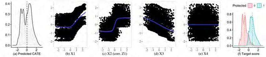
Figure 3: Estimated conditional balanced targetability (CBT) using BEAT. Figure (a) shows
               the distribution of CBT, (b) through (e) show the relationships between unprotected characteristics X1
               through X4 (x-axis) and predicted CBT (y-axis), and (f) shows the distribution of CBT by different
               values of the protected attribute Z1 .

3     Method

3.1    Overview
The primary goal of BEAT is to identify (observed) heterogeneity across individuals that is unre-
lated to their protected attributes. That heterogeneity is then used to implement targeted alloca-
tions that are, by construction, balanced on the protected attributes. Furthermore, we want our
method to be as general as possible, covering a wide variety of personalization tasks. In the example
presented in Section 2, we were interested in identifying differences in the effect of a treatment Wi
on an outcome Yi . This is commonly the case for personalized medicine, targeted firm interven-
tions, or personalized advertising. In other cases (e.g., approving a loan based on the probability
of default), the goal would be to extract heterogeneity on the outcome itself, Yi (e.g., Yi indicates
whether the individual will default in the future).

       We build on generalized random forests (GRF) (Wager and Athey 2018; Athey et al. 2019),
which are designed to efficiently estimate heterogenous outcomes. Generally speaking, GRF uses
forests as a type of adaptive nearest neighbor estimator and achieves efficiency by using gradient-
based approximations to specify the tree-split point. (See Athey et al. (2019) for details on the
method and https://github.com/grf-labs/grf for details on its implementation.) The key difference
between GRF and our method is the objective when partitioning the data to build the trees (and
therefore forests): Rather than maximizing divergence in the object of interest (either treatment
effect heterogeneity for causal forest or outcome variable for prediction forests) between the chil-
dren nodes, BEAT maximizes a quantity we define as “balanced divergence” which combines the
divergence of the outcome of interest (object from GRF) with a penalized distance between the
empirical distribution of the protected attributes across the children nodes.

                                                         8
Specifically, in the BEAT algorithm, trees are formed by sequentially finding the split that
maximizes the balanced divergence (BD) object:
ˆ 1 , C2 q ´ γDistpZ̄C |Xk,s , Z̄C |Xk,s q
BDpC1 , C2 q “ ∆pC (1)
loooomoooon 1 2
loooooooooooooooomoooooooooooooooon
GRF split BEAT added penalty
criterion
where C1 and C2 denote the children nodes in each split s, ∆pCˆ 1 , C2 q denotes the divergence in the
outcome of interest (as defined in equation (9) in Athey et al. (2019)7 ), γ is a non-negative scalar
denoting the balance penalty, which can be adjusted by the researcher (see discussion in section 3.2),
Dist is a distance function (e.g., Euclidean norm), and Xk,s is the splitting point for C1 and C2
at dimension k P K.8 When selecting splits to build a tree, Athey et al. (2019) optimizes the first
term of equation (1), indicated with “GRF split criterion,” and BEAT essentially adds a second
term to the equation, introducing a penalty when there are differences in the Z attributes between
the children nodes. Therefore, maximizing balanced divergence when sequentially splitting the
data ensures that all resulting trees (and hence, forests) are balanced with respect to the protected
attributes Z.
Once trees are grown by maximizing equation (1), we proceed exactly as GRF and use the
trees to calculate the similarity weights used to estimate the object of interest. More formally,
indexing the trees by b “ 1, . . . , B and defining a leaf Lb pxq as the set of training observations
falling in the same leaf as x, we calculate balanced weights α̃bi pxq as the frequency with which the
ith observation falls into the same leaf as x, and we calculate the conditional balanced targetability
score by combining the weights and the local estimate of the quantity estimated by GRF — i.e., the
treatment effect heterogeneity (τi ) for causal forest or expected outcome variable (µi ) for prediction
forests. For example, in the simplest case of prediction forest, we can express the conditional
balanced targetability (CBT) score as:
N
ÿ
CBT pxq “ α̃i pxqµ̂i (2)
i“1
řB 1
where α̃i pxq “ b“1 α̃b pxq and µ̂i is the leave-one-out estimator for E rYi | Xi “ xs.
B i
Note that the only difference between the CBT scores provided by BEAT and the estimates
provided by GRF are the similarity weights whereby α̃bi pxq (from BEAT) are balanced with respect
to Z, and αbi pxq from GRF do not depend on Z. For the special case in which variables X and Z
7
For brevity, we refer to the notation and expressions introduced in Athey et al. (2019)
8
To gain efficiency when computing Z̄Cc |Xk,s in each child c we pre-process the data. First, we split Xk into 256
equal bins and subtract the average of Z within the bin. Then, we take the average of Z for each splitting point Xk,s
and child node c to obtain Z̄Cc |Xk,s .
9are independent, maximizing equation (1) corresponds to maximizing ∆pC ˆ 1 , C2 q, exactly as GRF
does, and therefore CBTi pxq from equation (2) corresponds to the outcome of GRF, τ̂ pxq for causal
forests, and µ̂pxq for regression forests.
3.2 Efficiency/Balance trade-off
The penalty parameter γ in equation (1) determines how much weight the algorithm gives to
balance in protected attributes. Running BEAT while setting γ “ 0 would yield exactly the same
outcomes as running GRF without protected attributes. As γ increases, the imbalance in the
protected attributes would be reduced, but the main outcome to optimize may be lower as well.
Naturally, introducing an additional constraint in contexts where bias exists would necessarily
reduce efficiency while improving fairness. Because the penalty parameter in BEAT is flexible, one
can easily explore the efficiency/fairness trade-off of any particular context by adjusting the value
of γ. Figure 4 illustrates this trade-off using the illustrative example of Section 2.
The y-axis in the figure represents the efficiency of each method, measured as the value
obtained by personalization compared to the average random policy as described above, while the
x-axis captures the imbalance in protected attribute Z1 , which is the over-allocation proportion of
Z1 “ 1.
Figure 4: Efficiency/Balance trade-off for illustrative example.
Efficiency is the proportion increase in outcome compared to random allocation. Imbalance is the
Eucledian distance between the average value of the protected attribute (Z1 q) in treated and non-treated
units of each policy.
We compare causal forest (CF) with full data, causal forest without the protected attributes, and BEAT
with 0 ď γ ď 5. Select values of γ are reported.
10As illustrated in Section 2, when using the causal forest with the full data (case 1 above) both
the outcome and imbalance are the highest, at 75% over random and 0.70, respectively. Using a
causal forest without the protected attributes (case 2 above) yields lower results for both axes: 65%
and 0.42, respectively. Finally, the red line captures the performance of BEAT when using different
penalty weights γ and so captures the efficiency/balance trade-off in this particular example. If one
sets γ “ 0, the outcome is identical to that of case 2. Then, as γ increases (γ is increased by 0.05
intervals in the figure), there is a reduction in both outcome and imbalance, getting to a minimum
outcome of 38% when imbalance is reduced all the way to 0.9 Note that the relationship between
efficiency and balance in this example is not linear — for values of γ P r1.1, 1.25s BEAT can reduce
imbalance significantly without sacrificing too much efficiency. This gives the decision maker a
degree of freedom to allow a certain amount of imbalance while ensuring sufficient efficiency.
3.3 Simulation
We validate the effectiveness of BEAT by simulating a large variety of scenarios. Table 1 presents
simulation scenarios that illustrate BEAT’s performance compared to other personalization meth-
ods. Column (1) in the Table presents the Section 2 example. Then, in Column (2), we use this
baseline example and reduce the strength of the relationship between the protected attributes (Z)
and the unprotected attributes (X2 ). In Columns (3)-(4) we further vary the empirical relationship
between (X2 ,Z) and the variable of interest (τ ). Specifically, we allow both (X2 ,Z) to directly
affect τ , either with the same or the opposite sign. The Table compares the performance of BEAT
and other approaches including running GRF with and without the protected attributes (Cases 1
and 2 above), and running GRF using de-biased data X 1 , with X 1 “ X ´ fx pZq with fx being a
(multivariate) random forest with X as outcome variables and Z as features.
(1) (2) (3) (4)
Ò corr.; τ “ f pZq Ó corr.; τ “ f pZq Ó corr.; τ “ f pZ, Xi2 q Ó corr.; τ “ f pZ, ´Xi2 q
Imbalance Efficiency Imbalance Efficiency Imbalance Efficiency Imbalance Efficiency
CF-FD 100% 75% 100% 78% 100% 67% 100% 82%
CF-NP 61% 65% 4% 43% 34% 64% 110% 82%
De-biased 0% 31% 0% 34% 23% 61% 108% 80%
BEAT* 0% 38% 0% 37% 0% 37% 0% 44%
Table 1: Simulated scenarios: Comparing outcomes across methods
Reporting results comparing: CF-FD = CF with full data; CF-NP = CF without protected attributes;
De-biased uses regression forests to de-bias the data; BEAT is denoted with * to highlight that gamma is
set to maximum, yielding the most conservative estimates for efficiency and imbalance.
Imbalance is normalized to 100% for the imbalance obtained with CF-FD (e.g., in Column (1), CF-NP
generates 63% of the imbalance obtained when using the full data). Efficiency is measured as % increase
in outcome over random allocation.
9
Note that setting γ to values greater than 1.35 does not reduce the efficiency of the method, with 38% being the
lowest outcome obtained by the BEAT method.
11These scenarios illustrate several important patterns that highlight the benefits of the BEAT
framework compared to existing solutions. First, when the unprotected attributes do not directly
impact the variable of interest (Columns 1 and 2), de-biasing the X’s works almost as well as BEAT
— the imbalance is completely removed. However the outcome is also slightly less efficient compared
to BEAT. Second, comparing Columns 1 and 2, when the correlation between the protected and
unprotected attributes is relatively low, GRF without protected characteristics is almost as effective
as BEAT and de-biasing in removing the imbalance. Third, once the correlated variables impact the
variable of interest directly (Columns 3 and 4), de-biasing is no longer able to remove the imbalance,
while BEAT does. Further, when both unprotected and protected attributes impact the variable
of interest, but with opposite signs, both removing protected attributes and de-biasing the X’s
yield more imbalance compared to the baseline approach that uses all the data. From a practical
point of view, this insight is relevant because firms and organizations are increasingly eliminating
protected attributes from their databases (or are pressured to do so). Our analysis shows that doing
so could make things worse as there are cases when removing protected attributes (or trying to
de-bias data before using it for personalization) increases — rather than decreases — the imbalance
between protected and unprotected groups.
3.4 Experiment
We demonstrate the real-world applicability of our method using experimental data. As highlighted
in Table 1, the imbalance in outcomes depends on the strength of the relationships between pro-
tected and unprotected attributes as well as the underlying relationships between observables and
outcomes. Therefore, the goal of this analysis is twofold: (1) investigate the extent to which under-
lying correlations between “protected” and “unprotected” characteristics occur in real-world data,
and (2) explore whether those underlying relationships lead to imbalance against a “protected”
group, and if so, demonstrate how the BEAT framework mitigates the imbalance and generates
balanced outcomes when those relationships are ingrained in high-dimensional data, as is the case
in most real applications.
To that end, we ran an incentive compatible online experiment where 3,146 participants
were randomly assigned to different conditions of a marketing campaign akin to a situation where
some participants were offered a $5 discount and others were not (see SI Appendix A for details).
Participants were then asked to make a subsequent choice of buying from the company that offered
the coupon or the competitor. In addition, we collected behavioral and self-reported measures
about each participant (e.g., brand preferences, attitudes towards social issues, behavior in social
media sites) as well as demographic characteristics which are generally considered as protected
attributes (age, gender, and race) to explore the underlying correlations between unprotected and
protected attributes, and the relationship between these variables and the choice outcome.
12First, we explore the correlations between the protected attributes and other customer vari-
ables, for which we run a set of (univariate) regressions of each protected attribute on the (unpro-
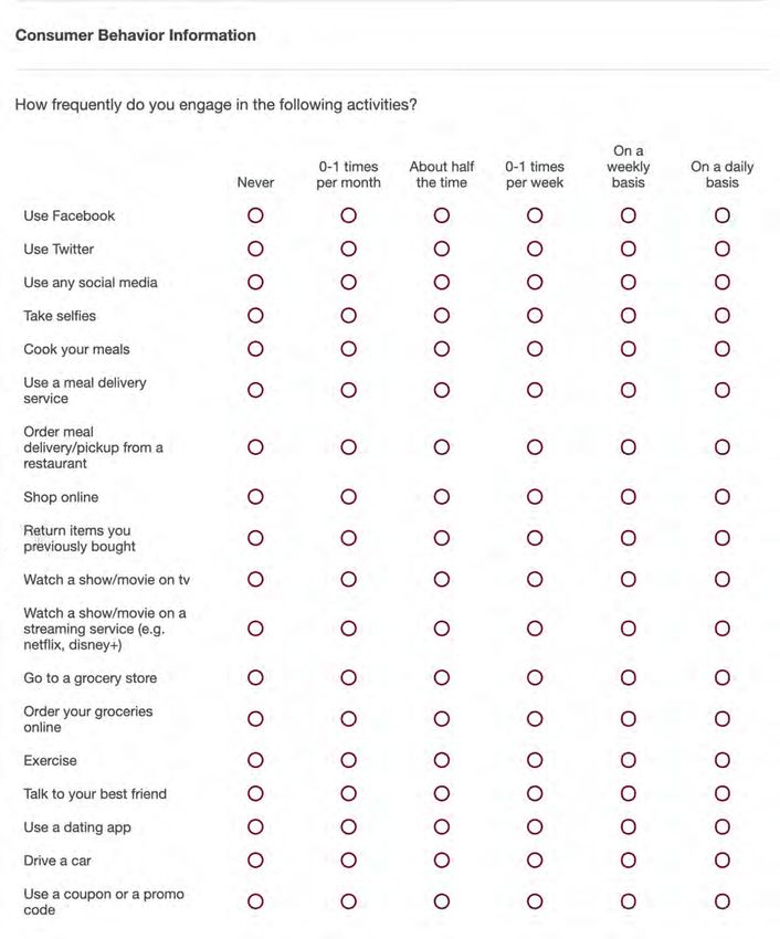
tected) variables. To illustrate the correlations, we report this analysis for the “activity” variables.10
Specifically, we use linear regression for age, and logistic regressions for gender (coded as non-male)
and race (coded as non-white). Figure 5 shows the coefficients from those regressions, revealing
that many of the non-protected attributes predict the ones that are protected. Note that most of
these activity-related variables capture very “seemingly innocent” behaviors such as how frequently
one cooks their own meals, or uses a dating app; behaviors that are easily captured by information
regularly collected by firms (e.g., past browsing activity). Importantly, the fact that these relation-
ships commonly occur in real life implies that, in cases where personalization leads to imbalance
in the protected attributes, simply removing those attributes from the data will not be enough to
mitigate such a bias.
Figure 5: Experimental data: Relationship between protected and unprotected at-
tributes
The figure shows regression coefficients (and 95% confidence intervals) of the protected attributes on
the activity-related variables. We use OLS regression for age, and logistic regression for non-male and
non-white. Blue bars indicate which regression coefficients are significantly different from zero at the
95% confidence level.
10
Please refer to the “Consumer Behavior Information” section in SI Appendix B for details about the collection
of the activity-related variables, and to the “Activity Frequency” section in SI Appendix C for the corresponding
summary statistics. These appendices include details about all variables included in the experiment.
13Second, we explore what would happened if the focal company used these data to design
personalized marketing policies. Specifically, we are interested in exploring whether a profit-
maximizing marketing campaign would lead to unbalanced policies (in the protected attributes)
and if so, how much bias would still remain even when those attributes are removed from the
data. Furthermore, we want to explore the performance of BEAT on the (real-world) marketing
example and demonstrate how BEAT can mitigate that unintended bias. Accordingly, we analyze
our experimental data emulating what a firm designing targeted campaigns would do in practice
(Ascarza 2018; Simester et al. 2020; Yoganarasimhan et al. 2020). Specifically, we randomly split
the data into train and test samples and use the training data to learn the optimal policy under
each approach. This corresponds to a firm running an experiment (or a pilot test) among a subset
of users to determine the optimal targeting policy. We then evaluate each policy using the test data,
mimicking the step when the firm applies the chosen policy to a larger population. We replicate
this procedure 100 times (using a 90/10 split for train and test samples) and report the average
outcomes of different methods in Table 2.11
Imbalance Efficiency
CF-FD 100% 2.0%
CF-NP 17% 1.8%
De-biased 20% 0.5%
BEAT (γ “ 3) 6% 1.8%
BEAT (γ “ 5) 5% 0.4%
BEAT (γ “ 8) 2% 0%
Table 2: Experimental data: Comparing outcomes across methods
Reporting results comparing: CF-FD = CF with full data; CF-NP = CF without protected attributes;
De-biased uses regression forests to de-bias the data; BEAT estimated with moderate and high penalties
for imbalance. Imbalance is normalized to 100% for the imbalance obtained with CF-FD with respect to
random allocation). Efficiency is measured as % increase in outcome over random allocation.
As can be seen in Table 2, BEAT preforms best in removing the imbalance, especially as we
increase the penalty. Unlike our simulated scenarios, the efficiency of any of the personalization
method is modest in this real-world setting.12 In turn, the efficiency fully dissipates as we remove
the imbalance, suggesting that all the value of personalization is driven by variables that are either
protected or related to those. Specifically, removing the protected attributes from the data still
results in positive levels of efficiency (1.8%), implying that there is incremental value to person-
alizing based on non-protected attributes. However, this method results in 17% imbalance, which
suggests that some of the variables that determine the allocation are related to protected attributes
(as illustrated in Figure 6 below). With BEAT, the imbalance is lowest, but the efficiency decreases
11
To calculate the efficiency and imbalance of the random policy, we select 50% of individuals in the test data to
target (at random) and compute the resulting outcomes. Then, we compute the efficiency and imbalance over the
random policy.
12
The finding that personalization may yield very little benefit in real settings is consistent with previous work
(Yoganarasimhan et al. 2020; Rafieian and Yoganarasimhan 2021).
14further, reaching 0%, suggesting that that there is little “inocent” variation (i.e., variation in the
data that is independent from protected attributes) to leverage for personalization. That is, in this
case, a firm concerned about imbalance may be better off by simply using a uniform policy rather
than personalizing the offers. Therefore, another way BEAT can be used is to help a decision maker
decide whether to use a uniform or a targeted policy.
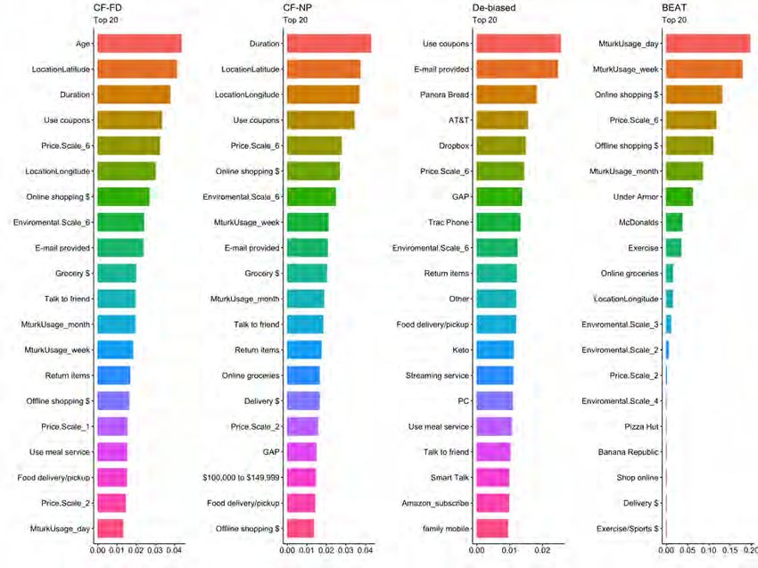
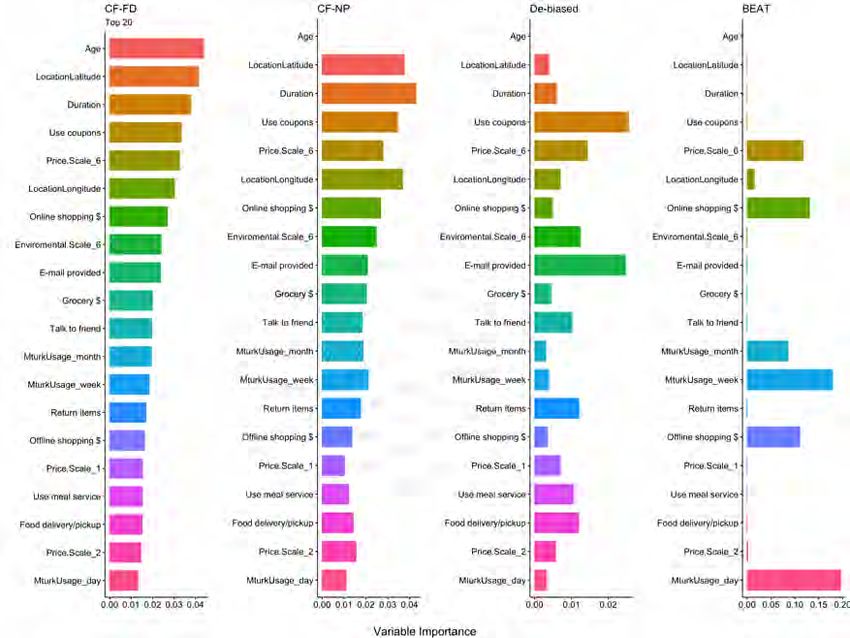
Finally, we explore in more depth the attributes that cause the imbalance in the most efficient
marketing allocation. We identify the 20 variables with the highest variable importance when
estimating the full causal forest,13 and then we examine their relative importance when applying
each of the other methods (Figure 6).14
Figure 6: Experiment results: Variable importance across methods.
The figure plots the variable importance of the top 20 variables for the causal forest with full data
(CF-FD), and the corresponding importance of these variables across the other methods: CF without
protected attributes (CF-NP), the De-biased method, and BEAT. Details about the experiment and the
different variables appear in SI Appendix A.
13
Variable importance indicates the relative importance of each attribute in the forest, and it is calculated as a
simple weighted sum of how many times each feature was split on at each depth when training the forest.
14
For completeness, we report the top 20 variables identified by each method in Figure S-1 of the SI Appendix.
15In the full causal forest, age (a protected attribute) is the most important variable, with
participant’s location, time spent responding to the experiment survey, and variables related to price
sensitivity (e.g., coupon usage, items on the price sensitivity scale, and spending across different
domains) also ranking among the high-importance variables. The relative importance of these
(unprotected) variables remains very similar when removing the protected attributes (CF-NP) —
where age is not used for personalization and therefore its importance is zero by construction.
In contrast, when using the De-biased method, where all the variables aside from age are still
used (albeit transformed to be independent from protected attributes), their importance varies
significantly compared to the previous two methods. Specifically, location and time spent on the
survey (duration) — variables likely to correlate with age — are less important, albeit still relatively
important. Finally, results from the BEAT method reveal that such variables should not be used
when training the model (i.e., splitting the trees), because doing so would create imbalance in
personalized policies. In other words, consistent with the results presented in Figure 5, many of
the unprotected variables used by the other methods were deemed to have a relationship with the
protected attributes, which then generated unintended imbalance in the other methods. That led
BEAT to eliminate these variables as a source of heterogeneity for personalization and use other
unprotected attributes instead.
4 Discussion
As personalized targeted policies become more prevalent, the risk of algorithmic bias and discrimi-
nation of particular groups grows. The more data used for personalization, underlying correlations
between protected and unprotected attributes are more likely to exist, thus generating unintended
bias and increasing the imbalance between targeted and non-targeted groups. As we have shown,
even existing methods of personalization that are supposed to tackle this issue tend to maintain — or
even exacerbate — imbalance between groups. This insight is especially important as firms imple-
ment policies that remove protected attribute or “de-bias” the data, presuming that doing so will
remove unintended biases or eliminate the risk of discrimination in targeted policies.
We introduce BEAT, a method to leverage unprotected attributes for personalization, while
maintaining balance between protected groups, thus eliminating bias. This flexible method can be
applied to multi-dimensional protected attributes, and to both discrete and continuous explanatory
and outcome variables, making it implementable in a wide variety of empirical contexts. Through
a series of simulations and also using real data, we show that our method indeed reduces the
unintended bias while allowing for benefits from personalization. We also demonstrate how our
method can be used to evaluate the trade-off between personalization and imbalance, and to decide
when a uniform policy is preferred over a personalized one.
16The goal of BEAT is to balance the allocation of treatments among individuals with respect
to protected attributes. When doing so, it may impact the efficiency of the outcome of interest
and/or increase prediction errors (compared to personalization algorithms that are built to optimize
these metrics). Moreover, the BEAT approach uses the distribution of protected attributes in the
data when balancing allocation to determine “fair” outcomes. Therefore, decision makers that
have different fairness or optimization objectives in mind may choose a different approach when
allocating treatments. As has been documented in the literature (Friedler et al. 2021; Miconi 2017),
different fairness definitions often yield different outcomes, and practitioners and researchers should
have a clear objective in mind when designing “fair” policies. In line with this issue, BEAT proposes
a solution to ensure equality of treatment among groups as well as individual parity, which may not
always be the desired outcome. This suggests future avenues for researchers to develop solutions
that allow optimization of multiple goals.
Regarding the applicability of BEAT, in our simulations and experiment, we used examples
in which the allocation was based on the treatment effect. Therefore, these included an initial phase
of random assignment into treatment,15 and we utilized BEAT in the second stage for inference.
It is important to note that BEAT can easily be applied to any type of allocation decision that
is based on prediction algorithms (such as medical treatments, hiring decisions, lending decisions,
recidivism prediction, product recommendations, or dynamic pricing), even without the random
assignment stage. For example, let us consider the case of lending when the decision depends on
the individual’s probability of default. In that case, the BEAT framework is applied to simple
regression forests (instead of causal forest) and similarly mitigates potential discrimination in the
allocation of loans.
To conclude, BEAT offers a practical solution to an important problem and allows a decision
maker to leverage the value of personalization while reducing the risk of disproportionately targeting
individuals based on protected attributes.
References
Agarwal, A., Beygelzimer, A., Dudik, M., Langford, J., and Wallach, H. (2018). A reductions
approach to fair classification. In Dy, J. and Krause, A., editors, Proceedings of the 35th Interna-
tional Conference on Machine Learning, volume 80 of Proceedings of Machine Learning Research,
pages 60–69. PMLR.
Ascarza, E. (2018). Retention futility: Targeting high-risk customers might be ineffective. Journal
of Marketing Research, 55(1):80–98.
15
Like GRF, BEAT does not require randomized assignment to be present prior to analyzing the data. It can be
used with observational data as long as there is unconfoundedness.
17Athey, S., Tibshirani, J., Wager, S., et al. (2019). Generalized random forests. Annals of Statistics,
47(2):1148–1178.
Athey, S. and Wager, S. (2021). Policy learning with observational data. Econometrica, 89(1):133–
161.
Castelnovo, A., Crupi, R., Greco, G., and Regoli, D. (2021). The zoo of fairness metrics in machine
learning. arXiv preprint arXiv:2106.00467.
Cowgill, B. (2019). Bias and productivity in humans and machines. SSRN Electronic Journal
3584916.
Cowgill, B. and Tucker, C. E. (2020). Algorithmic fairness and economics. SSRN Electronic Journal
3361280.
Donini, M., Oneto, L., Ben-David, S., Shawe-Taylor, J., and Pontil, M. (2020). Empirical risk
minimization under fairness constraints. arXiv preprint arXiv:1802.08626.
Feldman, M., Friedler, S. A., Moeller, J., Scheidegger, C., and Venkatasubramanian, S. (2015).
Mitigating unwanted biases with adversarial learning. In Proceedings of the 21th ACM SIGKDD
International Conference on Knowledge Discovery and Data Mining, pages 259––268. Association
for Computing Machinery.
Friedler, S. A., Scheidegger, C., and Venkatasubramanian, S. (2021). The (im)possibility of fairness:
Different value systems require different mechanisms for fair decision making. Communications
of the ACM, 64(4):136–143.
Goh, G., Cotter, A., Gupta, M., and Friedlander, M. (2016). Satisfying real-world goals with
dataset constraints. arXiv preprint arXiv:1606.07558.
Hahn, P. R., Murray, J. S., Carvalho, C. M., et al. (2020). Bayesian regression tree models for causal
inference: Regularization, confounding, and heterogeneous effects (with discussion). Bayesian
Analysis, 15(3):965–1056.
Horvitz, D. G. and Thompson, D. J. (1952). A generalization of sampling without replacement
from a finite universe. Journal of the American statistical Association, 47(260):663–685.
Johndrow, J. E. and Lum, K. (2019). An algorithm for removing sensitive information: Application
to race-independent recidivism prediction. Annals of Applied Statistics, pages 189–220.
Kamishima, T., Akaho, S., Asoh, H., and Sakuma, J. (2012). Fairness-aware classifier with prejudice
remover regularizer. In Flach, P. A., De Bie, T., and Cristianini, N., editors, Machine Learn-
ing and Knowledge Discovery in Databases, pages 35–50, Berlin, Heidelberg. Springer Berlin
Heidelberg.
Kennedy, E. H. (2020). Optimal doubly robust estimation of heterogeneous causal effects. arXiv
preprint arXiv:2004.14497.
Kleinberg, J., Ludwig, J., Mullainathan, S., and Sunstein, C. R. (2020). Algorithms as discrimina-
tion detectors. Proceedings of the National Academy of Sciences, 117(48):30096–30100.
18Lambrecht, A. and Tucker, C. E. (2019). Algorithmic bias? an empirical study of apparent gender-
based discrimination in the display of stem career ads. Management Science, 65(7):2966–2981.
Litman, L., Robinson, J., and Abberbock, T. (2017). Turkprime.com: A versatile crowdsourcing
data acquisition platform for the behavioral sciences. Behavior Research Methods, 49(2):433–442.
Miconi, T. (2017). The impossibility of “fairness”: A generalized impossibility result for decisions.
arXiv preprint arXiv:1707.01195.
Nie, X., Brunskill, E., and Wager, S. (2021). Learning when-to-treat policies. Journal of the
American Statistical Association, 116(533):392–409.
Pandey, A. and Caliskan, A. (2021). Disparate impact of artificial intelligence bias in ridehailing
economy’s price discrimination algorithms. AAAI/ACM Conference on Artificial Intelligence,
Ethics, and Society (AAAI/ACM AIES 2021).
Pope, D. G. and Sydnor, J. R. (2011). Implementing anti-discrimination policies in statistical
profiling models. American Economic Journal: Economic Policy, 3(3):206–31.
Rafieian, O. and Yoganarasimhan, H. (2021). Targeting and privacy in mobile advertising. Mar-
keting Science, 40(2):193–218.
Raghavan, M., Barocas, S., Kleinberg, J., and Levy, K. (2020). Mitigating bias in algorithmic
hiring: Evaluating claims and practices. In Proceedings of the 2020 conference on fairness,
accountability, and transparency, pages 469–481.
Simester, D., Timoshenko, A., and Zoumpoulis, S. I. (2020). Efficiently evaluating targeting policies:
Improving on champion vs. challenger experiments. Management Science, 66(8):3412–3424.
Wager, S. and Athey, S. (2018). Estimation and inference of heterogeneous treatment effects using
random forests. Journal of the American Statistical Association, 113(523):1228–1242.
Williams, B. A., Brooks, C. F., and Shmargad, Y. (2018). How algorithms discriminate based on
data they lack: Challenges, solutions, and policy implications. Journal of Information Policy,
8:78–115.
Woodworth, B., Gunasekar, S., Ohannessian, M. I., and Srebro, N. (2017). Learning non-
discriminatory predictors. In Proceedings of the 2017 Conference on Learning Theory, volume 65
of Proceedings of Machine Learning Research, pages 1920–1953. PMLR.
Yoganarasimhan, H., Barzegary, E., and Pani, A. (2020). Design and evaluation of personalized
free trials. SSRN Electronic Journal 3616641.
Zafar, M. B., Valera, I., Rodriguez, M. G., and Gummadi, K. P. (2017). Fairness constraints: Mech-
anisms for fair classification. In Proceedings of the 20th International Conference on Artificial
Intelligence Statistics (AISTATS), pages 962––970.
Zhang, B. H., Lemoine, B., and Mitchell, M. (2018). Mitigating unwanted biases with adversarial
learning. In Proceedings of the 2018 AAAI/ACM Conference on AI, Ethics, and Society, pages
335––340.
19SI Appendix
A Further details about the experiment
A.1 Experimental design
Consider Domino’s Pizza as an example of a firm which could leverage their customer data to
increase the profitability of their marketing campaigns via personalization.1 Our ideal data would
have replicated as closely as possible what Domino’s Pizza would do in this case, i.e., randomly
send coupons to individuals and then measure and compare revenues and profits among those who
x
received a coupon and those who did not, and design a targeting policy accordingly. However, due
to the request to have access to detailed data including protected characteristics, a collaboration
di
with a firm was not possible. Instead, we set up an experiment such that all individuals were offered
$5 gift cards, and those in the treatment condition were offered a higher value ($10) of the focal
company’s gift card (replicating a $5 coupon). Specifically, the experiment consisted of a simple
n
choice manipulation task akin to what companies call an “A/B Test.” Individuals in the control
condition were offered a choice between $5 gift cards to Panera Bread and to Domino’s Pizza. In
pe
the treatment condition, participants were given a similar choice, but the Domino’s Pizza gift card
had a value of $10. To ensure truth-telling, the experiment was incentive-compatible—participants
were informed that one of every 100 participants will receive the gift card of their choice.
In addition to the main experimental choice manipulation, we collected detailed information
Ap
from participants about their brand preferences and consumption behaviors, similar to data a
company may collect or infer about its consumers: (i) brands in four categories (sportswear, apparel,
chain restaurants, and technology and social media companies) are rated on a three-point scale of
dislike, indifferent, and like; (ii) consumption behaviors such as coupon usage, Facebook usage,
exercise frequency, and other daily behaviors are rated on a six-point scale between “never” and
“on a daily basis;” (iii) other general information such as subscription services usage, operating
system, mobile service provider, dietary restrictions, and mTurk usage frequency; and (iv) other
1
Any firm that collects individual-level customer data and that has the capability to personalize its marketing
promotional activity would be a valid candidate.
S-1personal information such as monthly budget of various activities, pet ownership, price sensitivity
scale, environmentally friendliness scale, education level, and monthly income. Those variables are
used in the analysis as the unprotected attributes. Some of these may turn out to be “guilty”
(i.e., related to the protected attributes) while others are “innocent” (unrelated to the protected
attributes). We also collected information from the Qualtrics survey session (each participant’s
latitude and longitude, and the duration of time they spent responding to the survey). Finally, we
also collected protected demographic attributes–gender, race, and age. We collected three different
types of protected attributes in order to maximize the potential relationships between those and
x
the unprotected attributes. The gift card task appeared at the end of the survey: after participants
learned about the lottery, the next page presented the experimental stimuli and asked them to
di
make a choice, and the final page asked them to enter their email to receive the gift card. Section B
in the Web Appendix provides the full details of the study.
The back story for the study was that we were conducting research to better understand
n
consumer preferences and choices, and the gift cards were presented as additional compensation for
the study. Via Cloud Research (Litman et al. 2017), we recruited 3,205 participants2 who completed
pe
the survey. In addition to the gift card of their choice that 32 of the participants received, each
participant was compensated $1.30 for their participation in the seven to eight minutes survey, a
standard market rate at the time the study was conducted. Seven participants did not complete
the gift card selection task and an additional 52 did not fill out their demographic information.
Therefore, the final sample included 3,146 participants.
Ap
A.2 Experimental results
In this subsection, we first present summary statistics of the data. We then calculate the effect of
the $10 gift card treatment in our experiment using a simple regression to demonstrate the average
2
To calculate the required sample size, we first ran a pretest with 100 participants in each condi-
tion. Using a linear regression, we observed a statistically significant main effect of an increase Domino’s
Pizza choice. We also saw some (not statistically significant) interactions between some of the pro-
tected variables and the treatment. We thus recruited 16 times the sample size to identify interac-
tion effects. See https://statmodeling.stat.columbia.edu/2018/03/15/need-16-times-sample-size-estimate-interaction-
estimate-main-effect/ for more details.
S-2You can also read