Development of tools for coastal management in Google Earth Engine: Uncertainty Bathtub Model and Bruun Rule
←
→
Page content transcription
If your browser does not render page correctly, please read the page content below
Preprints (www.preprints.org) | NOT PEER-REVIEWED | Posted: 23 February 2021                           doi:10.20944/preprints202102.0513.v1

     Article

     Development of tools for coastal management in Google Earth
     Engine: Uncertainty Bathtub Model and Bruun Rule
     Lucas Terres de Lima 1,*, Sandra Fernández-Fernández 2, João Francisco Gonçalves 3, Luiz Magalhães Filho 4 and
     Cristina Bernardes 1

                                       1 CESAM - Centre for Environmental and Marine Studies, Department of Geoscience, University of Aveiro,
                                         Campus de Santiago, 3810-193 Aveiro, Portugal; cbenardes@ua.pt
                                       2 CESAM- Centre for Environmental and Marine Studies, Department of Physics, University of Aveiro,

                                         Campus de Santiago, 3810-193 Aveiro, Portugal; sandrafernandez@ua.pt
                                       3 CIBIO-InBIO, Research Center in Biodioversity and Genetic Resources, University of Porto, Campus de

                                         Vairão, Rua Padre Armando Quintas, 4485-661 Vairão, Portugal; joaofgo@gmail.com
                                       4 CESAM- Centre for Environmental and Marine Studies, Department of Environment and Planning, Univer-

                                         sity of Aveiro, Campus de Santiago, 3810-193 Aveiro, Portugal; luizlacerda@ua.pt
                                       * Correspondence: lucasterres@ua.pt

                                       Abstract: Sea-level rise is a problem increasingly affecting coastal areas worldwide. The existence
                                       of Free and Open-Source Models to estimate the sea-level impact can contribute to better coastal
                                       management. This study aims to develop and to validate two different models to predict the
                                       sea-level rise impact supported by Google Earth Engine (GEE) – a cloud-based platform for plan-
                                       etary-scale environmental data analysis. The first model is a Bathtub Model based on the uncer-
                                       tainty of projections of the Sea-level Rise Impact Module of TerrSet - Geospatial Monitoring and
                                       Modeling System software. The validation process performed in the Rio Grande do Sul coastal
                                       plain (S Brazil) resulted in correlations from 0.75 to 1.00. The second model uses Bruun Rule for-
                                       mula implemented in GEE and is capable to determine the coastline retreat of a profile through the
                                       creation of a simple vector line from topo-bathymetric data. The model shows a very high correla-
                                       tion (0.97) with a classical Bruun Rule study performed in Aveiro coast (NW Portugal). The GEE
                                       platform seems to be an important tool for coastal management. The models developed have been
                                       openly shared, enabling the continuous improvement of the code by the scientific community.

                                       Keywords: Sea-Level Rise; GIS; Open-Source Software; Modeling

                                       1. Introduction
                                            More than 30% of the world population lives in coastal areas - which are three times
                                       densely populated as inland areas and are increasing exponentially [1,2] - and between
                                       80% and 100% of the total population of more than half of coastal countries live within
                                       100 km from the coastline. Depending on the geologic, climatic, and oceanographic con-
                                       ditions, coastal zones may present a high risk of subsidence in some areas, storms expo-
                                       sure, tsunami, overwash and flood, coastal erosion, and regional sea-level fluctuations.
                                       All these phenomena are natural and contributed to model present-day coastlines.
                                       However, in the last seventy years, the effect of these drivers has increased in both in-
                                       tensity and frequency [3,4], and it is expected that this increasing trend keeps up in the
                                       future [5], being the anthropogenic forcing the main reason for the global average sea
                                       level rise since 1970 [6].
                                            The sea-level rise is a common problem that affects about 70% of coastal zones
                                       worldwide [7]. The Total Global Mean Sea-level (GMSL) rose 0.16 m between 1902 and
                                       2015. However, in the period 2006–2015, the GMSL rise rate was 3.6 mm yr–1, about 2.5
                                       times higher than in the period 1901–1990 (1.4 mm yr–1). The ice sheet and glacier con-
                                       tributions over the period of 2006–2015 were the most important sources of sea-level rise

               © 2021 by the author(s). Distributed under a Creative Commons CC BY license.
Preprints (www.preprints.org) | NOT PEER-REVIEWED | Posted: 23 February 2021               doi:10.20944/preprints202102.0513.v1

                                 (1.8 mm yr–1), exceeding the influence of the thermal expansion of ocean water (1.4 mm
                                 yr–1) [8].
                                       Sea-level rise is accelerated due to the contribution of ice loss from the Greenland
                                 and Antarctic ice sheets. Mass losses from the Greenland and Antarctic ice sheet doubled
                                 and tripled, respectively, in the years from 2007 to 2016 when compared with the period
                                 between 1997 and 2006 [7]. According to the Special Report on Climate Change and
                                 Oceans and the Cryosphere (SROCC) of Intergovernmental Panel on Climate Change
                                 (IPCC), the rate of global mean sea-level rise is projected to reach 4 mm yr-1 under a
                                 Representative Concentration Pathway – RCP 2.6 scenario and 15 mm yr–1 under RCP 8.5
                                 scenario in 2100 [6]. In a global scale, the sea-level changes are not spatially uniform. For
                                 example, in the United States of America, the estimated sea-level rise for New York City
                                 is 0.87 m whereas for the Los Angeles area is 0.57 m by the end of the century under the
                                 same RCP 8.5 scenario [7].
                                       Considering the dimension and complexity of sea-level rise hazards, the use of Ge-
                                 ographic Information Systems (GIS) to organize and to analyze the information produced
                                 about those issues is crucial to improve coastal management. Desktop GIS applications
                                 such as ArcGIS [9], gvSIG [10], Terraview [11], or QGIS [12] have traditionally been used
                                 in coastal management, but the exponential increase of Google Earth Engine [13] in terms
                                 of available data, and capability to address a considerable volume of datasets with high
                                 spatial resolution has become this powerful cloud-based platform capable to connect
                                 large-scale problems on coastal management in a new point of view.

                                 1.1. Google Earth Engine (GEE)

                                      The Google Earth Engine is a cloud-based platform that offers high-performance
                                 computing resources for processing geospatial data [13]. It provides access to an in-
                                 creasing amount of remotely obtained datasets through its Application Programming
                                 Interfaces (API) for JavaScript and Python languages, which decrease the complexity of
                                 laborious desktop-based computations [14].
                                      GEE use is growing very fast in the last few years. Several applications were de-
                                 veloped such as MapBiomas [15] that provide a historical dataset of land use maps;
                                 CoastSat that allows extracting coastlines from Landsat and Sentinel images [16]; and the
                                 extraction of bathymetry from Sentinel 2 images [17]. One of the best benefits of creating
                                 models on GEE is the possibility to work efficiently and quickly in a large scale. These
                                 advantages can be integrated into scripts (based on GEE API) by implementing modeling
                                 frameworks and creating new tools and analysis methodologies, which can improve new
                                 knowledge and its application.

                                 1.2. The Uncertainty Bathtub Model (uBTM)

                                      The simple Bathtub method is a GIS technique that shows the areas below a specific
                                 elevation level as being flooded, like a bathtub or single value water surface [18]. Based
                                 on the former, the Uncertainty Bathtub Model (uBTM) [19] is a modified version of this
                                 technique that combines the uncertainty of sea-level projections and the vertical error of a
                                 Digital Elevation Model (DEM). Based on the Terrset Sea-level Impact tool [20], the
                                 model defines the probability of the sea-level to flood a considered zone, using the level
                                 of uncertainty associated with the DEM and the sea-level rise projections.

                                 1.3. Brunn Rule for GEE Model (BRGM)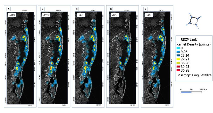
Preprints (www.preprints.org) | NOT PEER-REVIEWED | Posted: 23 February 2021                doi:10.20944/preprints202102.0513.v1

                                       The Brunn Rule for GEE Model (BRGM) [21] is based upon a formula created to es-
                                 timate the retreat of sandy beaches coastline in response to sea-level changes [22]. The
                                 Bruun Rule has some limitations, and its application requests precaution due to the sim-
                                 plicity of the formula; the equation does not include some essential variables such as ex-
                                 treme washover events, changes in sediment budget and anthropic action. However, the
                                 formulation shows accurate results in its applications history [23,24], and allows to obtain
                                 better results than those produced by modern models, such as the Profile Translation
                                 Model (PTM) [25].

                                       The main objective of this work is to explore the potential of GEE as support for two
                                 models - uBTM and BRGM - and its validation in the context of coastal management
                                 problems. The uBTM model uses the uncertainties of sea-level projections and the verti-
                                 cal digital elevation model error to create a coastal flooding scenario. The BRGM model is
                                 based on the Bruun Rule equation that generates a tool capable of determining the coast-
                                 line retreat in a coastal stretch.

                                 1.4. Study Sites
                                       The models were applied and validated using a morphological dataset of the
                                 southern Rio Grande do Sul, Brazil and of a region located in the northwest coast of
                                 Portugal.
                                       The Rio Grande do Sul coastal plain (RSCP) in the south of Brazil was chosen to
                                 validate the Uncertainty Bathtub Model (uBTM) (Figure 1 - A). The RSCP is characterized
                                 by an extensive NE-SW sandy barrier system of 620 km of length and a great variety of
                                 environments associated [26]. The coast is wave-dominated, and tides have a subordi-
                                 nated role in coastal hydrodynamics and present a mean amplitude of 0.5 m and a
                                 maximum of 1.2 m. The wave climate is dominated by two-wave propagation patterns,
                                 one composed of S-SE swell waves of higher amplitude and longer periods; the second
                                 comprising local generated waves, with shorter periods and a predominant E-SE direc-
                                 tion. Swell waves have a mean significant wave height of 1.5 m and periods of 12 s. Sea
                                 waves are characterized by a mean significant wave height of 1 m and a mean period of 8
                                 s [27].
                                       The continental shelf is wide (100 to 200 km), shallow (100 to 140 m) and slightly
                                 sloping (0.02° to 0.08°) [26]. Differences in width, slope and topographic features along
                                 the coastal region are a result of reworking action related to glacio-eustatic variations that
                                 occurred during the Quaternary [28]. The barrier system was formed in the last 7 Ka
                                 controlled by both sediment supply along the coast and morphology; coastal embayment
                                 promote the development of regressive barriers and steeper coastal slopes are dominated
                                 by transgressive barriers [29].
                                       Despite some erosional hotspots near the cities of Hermengildo [30], Rio Grande
                                 [31], Tramandaí [32], mainly due to human activities or extremes events ocurrence, the
                                 coastline shows in general a stable or accretionary trend [30,33] (Figure 1 - A).

                                      The second site considered, in order to validate the Bruun Rule for GEE Model
                                 (BRGM), is located in the northwest coast of Portugal (Figure 1 - B). The stretch is situated
                                 south of the Aveiro lagoon entrance and is morphologically characterized by a sandy
                                 barrier extending in NNE–SSW direction. Nowadays, this area is highly vulnerable to
                                 erosion due to the very low and flat topography, combine with high wave conditions and
                                 a meso-tidal regime [34]. The sector considered, from Barra to Poço da Cruz beaches, is
                                 backed by a degraded foredune ridge partially destroyed by erosive processes and re-
                                 placed by sand dykes. In general, the beaches show pronounced seasonal behavior, with
                                 a range of morphodynamical states. This variation reveals the important exchange of
                                 sediments between the upper and lower foreshore [35]. Despite this cross-shore
                                 transport, significant littoral drift causes major alongshore motion of sediments along the
                                 southward direction [36]. However, the presence of several cross-shore structures (jetties
                                 and groins) contributes to changes in the sediment transport patterns.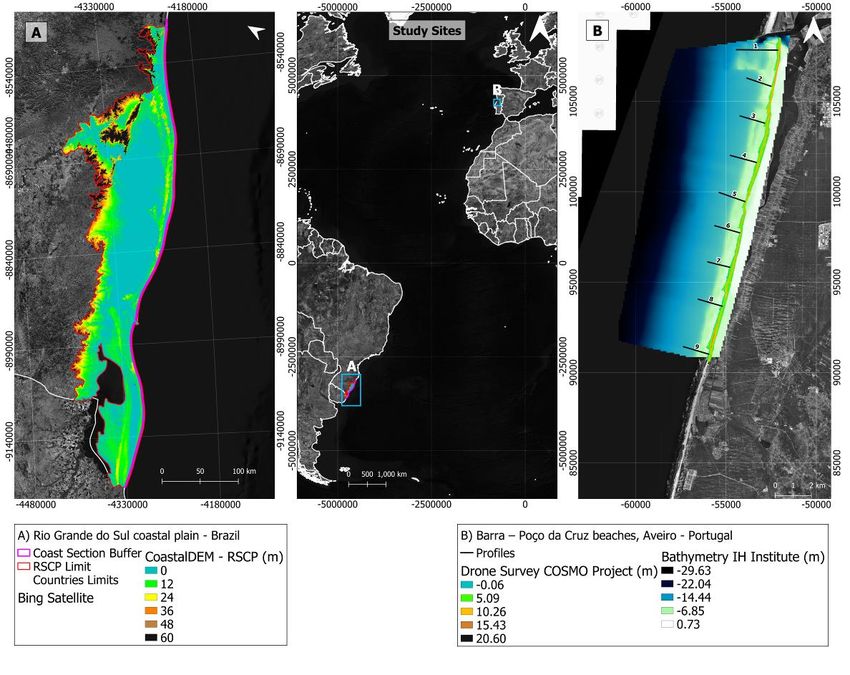
Preprints (www.preprints.org) | NOT PEER-REVIEWED | Posted: 23 February 2021                        doi:10.20944/preprints202102.0513.v1

                                          The coast is exposed to highly energetic waves from WNW–NNW [37]. In maritime
                                     summer (June to September) significant wave heights and mean periods are less than 3 m
                                     and 8 s, respectively. During winter and transitions periods, the mean significant wave
                                     heights and periods exceed 3 m (most common values of 3–4 m) and 8 s (most frequent
                                     mean periods of 8–9 s), with storms defined by a mean significant wave height greater
                                     than 5 m (often exceeding 7 m) and mean wave periods of 13 s, which can reach maxi-
                                     mum 18 s [38]. The average values for the spring and neap tidal ranges are 2.8 m and 1.2
                                     m, respectively.

                                          Despite the considerable differences between the two study sites, regarding the ge-
                                     ological, climatic, and oceanographic frameworks, both are sensitive areas to trigger
                                     events, e.g., storms and sea-level changes.

     Figure 1. Study sites: A) Rio Grande do Sul coastal plain - Brazil; B) South Aveiro lagoon entrance (Barra – Poço da Cruz strecht) -
     Portugal.

                                     2. Materials and Methods

                                     2.1. Uncertainty Bathtub Model

                                          The model was entirely implemented on the GEE using the JavaScript API. The
                                     model exams the uncertainty of sea-level rise projections with vertical errors in the DEM,
                                     creating a frequency from 0 to 100%, which indicates the probability of a specific area to
                                     be affected by sea-level rise (Figure 2 - a). The model assumes the lowest vertical error of
                                     a DEM and the highest sea-level rise projection (Figure 2 – b). The areas that appear
                                     emerged are considered locals with 0% of probability to be affected by sea-level rise
                                     flooding. On the other hand, a region has a 100% probability of being submerged when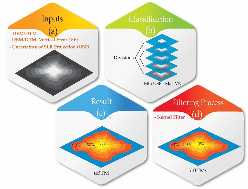
Preprints (www.preprints.org) | NOT PEER-REVIEWED | Posted: 23 February 2021               doi:10.20944/preprints202102.0513.v1

                                  the maximum error of DEM elevation is compared with the lowest sea-level rise projec-
                                  tion and the area appears submerged, even with optimistic settings (Figure 2 - c).

     Figure 2. a) Model inputs: DEM/DTM in raster format, vertical error of DEM/DTM, and uncertainty of SLR. b) Classi-
     fication process: maximum values of uncertainty of SLR projection with minimum vertical error of DEM/DTM, and a
     minimum of uncertainty of SLR with maximum vertical error of DEM/DTM and created other combinations of these
     scenarios by divisions. c) Result: all scenarios grouped into a single raster classified from 0% to 100% named uBTM. d)
     Filter process (optional) is applied a Kernel filter on uBTM creating a smoothed uBTM (uBTMs).

                                       The uBTM passed through a filtering process with different Kernel Filters, in order to
                                  choose the best option to smooth the data and to reduce both the pixelization and the
                                  image grain for a better delimitation of the waterline boundaries. All 3x3 Kernel Filters
                                  available on GEE (i.e. Cross, Plus, Gaussian, Diamond, Circle, Square, Octagon, Cheby-
                                  shev, Euclidean, and Manhattan) were tested and compared. The geometric aspect of the
                                  circular Kernel Filter seems more adequate for the waterline shapes of the study area.
                                  However, this filter can be easily changed on the code and to be selected the one that is
                                  more appropriate to the coastal characteristics (for example, a square filter is reasonably
                                  proper in the case of rocky cliff coasts). The result of the uBTM combined with the fil-
                                  tering process is called the uncertainty Bathtub Model smoothed (uBTMs) (Figure 2 – d).

                                  2.2 uBTM Validation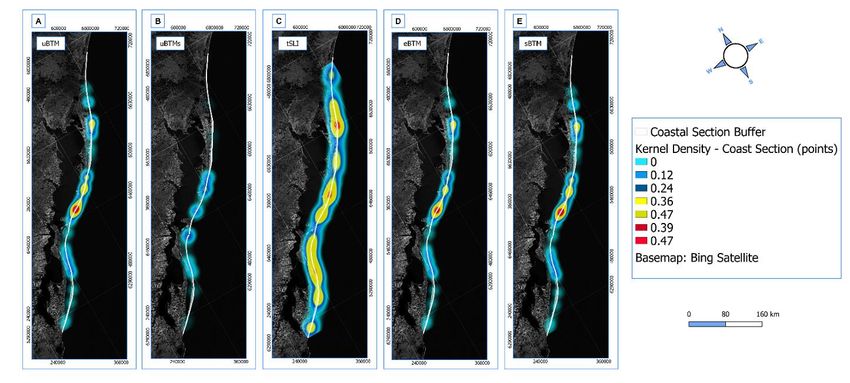
Preprints (www.preprints.org) | NOT PEER-REVIEWED | Posted: 23 February 2021                doi:10.20944/preprints202102.0513.v1

                                       The validation of the uBTM consists of performing a comparison between three
                                 similar GIS models (i) Simple Bathtub Model (sBTM), (ii) Enhanced Bathtub Model
                                 (eBTM), and (iii) Terrset Sea-level Impact (tSLI), which are briefly described below.
                                       The sBTM is a user-defined static inundation water level that does not consider ei-
                                 ther the hydrological framework or physical barriers.
                                       The eBTM includes a roughness coefficient and the beach slope, to perform a more
                                 realistic representation of the area and coastal flooding conditions. The eBTM needs the
                                 surface roughness coefficient as input [39]. The surface roughness acts as a critical varia-
                                 ble that influences the water movement. In the present case, the study region (RSCP) is
                                 characterized by mainly sandy substrate in the first meters above the surface [40–44] and
                                 according to [45] sands are characterized by a uniform roughness coefficient of 1.
                                       The tSLI yields the effect of a sea-level rise integrating both the uncertainties of the
                                 projection and the DEM, using a PCLASS algorithm, which produces a probability image
                                 where values are between zero and one [20].
                                       The calculation of the area by itself is not a good indicator of the similarity between
                                 the models because it ignores the spatial distribution. For this reason, a different meth-
                                 odology was developed allowing the quantification of spatial differences to check spatial
                                 similarities between models.
                                       Several algorithms, including Artificial Intelligence, use heatmaps and statistical
                                 analyses to recognize objects and identify differences between images [46–48]. The
                                 method used to quantify the similarity of the spatial distribution consists of transforming
                                 the pixels values of model into a density map and applying a correlation matrix to assess
                                 the similarities and their distribution. An ArcMap graphical model was created to select
                                 only the impact by using the Extract by Mask, a tool that cuts the raster cells related to the
                                 area defined by a polygon [9]. In the case of uBTM, uBTMs and tSLI - that show the
                                 impact from 0 to 100% - 50% is the point that expresses the value of sea-level on DEM
                                 without the influence of vertical error and uncertainties of sea-level projections. The use
                                 of the same values for sBTM and eBTM allows comparing both models. The process to
                                 extract the area below 50% is represented in the graphical model by the Raster Calculator
                                 Tool, which allows to create and perform a map algebra expression that results in an
                                 output raster [9]. After that, the affected area of all models is transformed into points by
                                 the Raster to Points Tool. Then, it is applied the Kernel Density tool to create a heatmap of
                                 pixel changes for each model (Appendix A).
                                       It was necessary to remove the effect of lagoon areas (in the case of RSCP) and un-
                                 derstanding the spatial distribution near to the coastline. For this reason, the same pro-
                                 cedure (Extract by mask > Raster to Point > Kernel Density) was performed by creating a
                                 small sector through a buffer area of 500 m from the coastline vector. The final step was
                                 applied the Raster Correlations and Summary Statistics of SDM Toolbox v.2.4 [49], which
                                 creates a correlation matrix of the Kernel Density.
                                       The accuracy of the method was verified by using two accessible APIs for image
                                 comparison: i) DeepAI – Image Similarity [50] which uses an artificial neural network
                                 algorithm to identify the differences, ii) Resemble.js based on Visual Regression method
                                 [51]. The heatmap images of spatial distribution used for comparison were created by
                                 exporting from ArcGIS 10.6 the images of the Kernel Density in a white background. In the
                                 end, the density points created on ArcGIS, the outcomes of the process of DeepAI and
                                 Resemble.js, and the results of the area differences calculation were correlated using pyplot
                                 library and GoogleColab [52]. Matplotlib is a library for producing visualizations (i.e.
                                 charts) in Python [53]. The GoogleColab platform allows writing and executing python
                                 code through the web browser in a cloud environment [54].
                                       The DEM used to perform the analysis was the CoastalDEM Free Version (resolu-
                                 tion of 90 m), a product created with a multilayer perceptron (MLP) artificial neural
                                 network to reduce the vertical error of Shuttle Radar Topography Missions (SRTM) to ca.
                                 2.5 m [54].
                                       The values of sea-level rise were extracted from the regional data of Special Report
                                 on the Ocean and Cryosphere in a Changing Climate (SROCC) [5] under Representative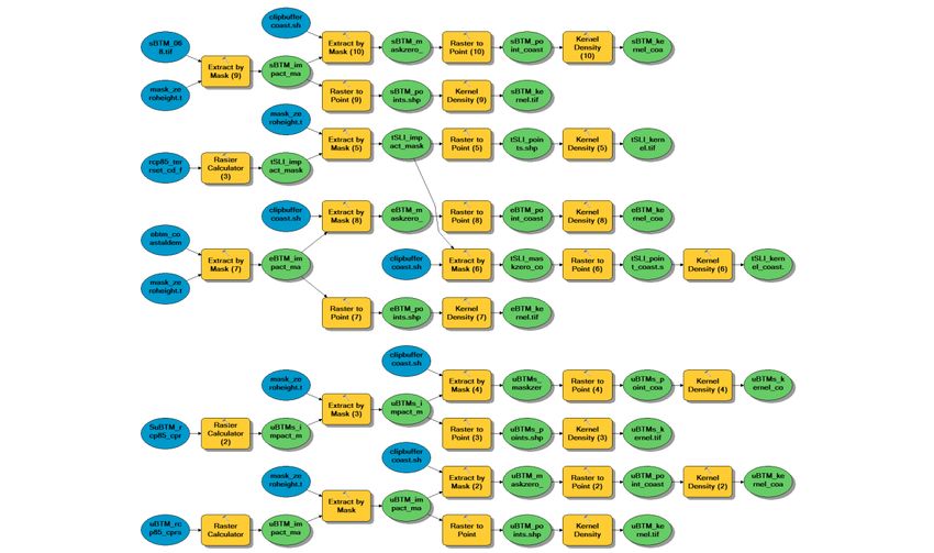
Preprints (www.preprints.org) | NOT PEER-REVIEWED | Posted: 23 February 2021               doi:10.20944/preprints202102.0513.v1

                                 Concentration Pathway-RCP 8.5. The value adopted is 0.68 m with the uncertainties of
                                 0.50 m to 0.90 m, for the period 2081-2100.

                                 2.3. Bruun Rule implementation on Google Earth Engine

                                       The Bruun formula [22] uses the berm height, the horizontal length after the berm
                                 ridge towards the backshore, or the beach face [55]. If the profile does not have a berm,
                                 the dune foot is considered. The code developed on GEE requires the sea-level rise pro-
                                 jection, DEM (raster format) of topography and bathymetry (Figure 3 – a) in order to
                                 create the topo-bathymetric profile, i.e. a line that allows obtain the values of the berm
                                 height and depth of closure (Figure 3 – b). After that, Equation 1 was used with the values
                                 extracted from the created line. The displacement representation in the future is repre-
                                 sented by using a simple buffer, with the extreme edge of the polygon being the final
                                 position of the coastline (Figure 3 - c).

                                      R=S(W/h+B)                                                                          (1)

                                       Bruun’s classic equation where R is the coastline retreat, S is the predicted sea-level
                                 rise, W is the profile length; h is the depth of closure and B the berm elevation.

                                      In the last years, modifications to the original Bruun equation were proposed by [56]
                                 in order to incorporate the landwards transport, and [57], that included the contributions
                                 of the cross and longshore sedimentary processes and the sediment budget (Appendix B).
                                 These variables were included in the code, but its precision was not evaluated in the
                                 present study.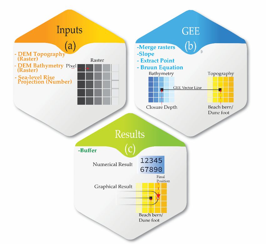
Preprints (www.preprints.org) | NOT PEER-REVIEWED | Posted: 23 February 2021                         doi:10.20944/preprints202102.0513.v1

     Figure 3. a) Model inputs: DEM of topography and DEM of bathymetry, both in raster format, and the value number of sea-level

     rise projection. b) Google Earth Engine: the rasters are merged and to calculate the slope. The closure depth and beach berm values

     are extracted directly from GEE. c) Numerical and graphical result, in the last case symbolized by a buffer.

                                           In this study, the classic Bruun equation (Eq. 1) was applied on the Portuguese
                                      coastal stretch, between Barra and Poço da Cruz beaches (Aveiro region), using bathym-
                                      etry and UAV photogrammetry DEM data (Figure 1). The results were compared with
                                      [58]’s study, which performed a Bruun Rule analysis in the same region. Profiles for the
                                      GEE Model (BRGM) were created with the values detailed in this study. However there
                                      are some bathymetric and topographic differences between the profiles performed by
                                      [58] and the present analysis because it was necessary to adapt the length of some profiles
                                      to get similar values of height and depth. The topographic and bathymetric data used
                                      have two sources, the COSMO Program [59] (topography) with 1 m of spatial resolution
                                      and the Portuguese Hydrographic Institute [60] (bathymetry) with 82.4 m of spatial res-
                                      olution. Subsequently, a Spearman correlation analysis between the results of the GEE
                                      Bruun Rule and the previous study [58] was performed. After the validation process, was
                                      tested for the area a scenario of sea level rise of 1.21 m, considering the contribution of the
                                      ice sheets melting process (AIS = 60 cm) [61].

                                      3. Results
                                           The results section is divided in two subsections: i) the validation process of the
                                      Uncertainty Bathub Model (uBTM) and ii) Bruun Rule validation for Google Earth En-
                                      gine Model (BRGM) through Spearman correlation analysis and the example of the ap-
                                      plication of the BRGM under a climate change scenario.

                                      3.1. uBTM Validation
                                           The subsection presents the results of the comparison of the areas between the dif-
                                      ferent models, and those obtained with the spatial similarity using Kernel Density and
                                      machine learning APIs.

                                      3.1.1. Comparison of the areas between models

                                            In Figure 4, the red color shows the areas with more than 50% of probability to be
                                      affected by a climate change scenario. The results are very similar in all the models per-
                                      formed, which means the outcomes of uBTM and uBTMs are coherent (Figure 4 – A and
                                      B). The regions in red color correspond to the total results of eBTM and sBTM (Figure 4 –
                                      D and E). Additionally, it is possible to observe the result of the Kernel filter smooth effect
                                      by using the uBTMs (Figure 4 - B, small frame). Besides, the Terrset Sea-level Impact
                                      (tSLI) showed the different spatial distribution of areas from 0 to 40% of impact (Figure 4
                                      – C).
Preprints (www.preprints.org) | NOT PEER-REVIEWED | Posted: 23 February 2021 doi:10.20944/preprints202102.0513.v1
Figure 4. Rio Grande coastal plain impact results. A) Uncertainty Bathtub Model (uBTM). B) Uncertainty Bathtub Model smoothed
(uBTMs). C) Terrset Sea-Level Impact (tSLI). D) Enhanced Bathtub Model (eBTM) in red. E) Simple Bathub Model (sBTM) in red.
The tSLI yields the most significant area affected, but the difference between tSLI
and uBTM represents only 0.63% of the total area of Rio Grande do Sul coastal plain
(RSCP) and 2.99% of the coastal stretch or section (CS). Furthermore, the total areas ob-
tained by the uBTM and sBTM are similar (Figure 5). In the coast section, the eBTM,
uBTM and sBTM show also similar results.Preprints (www.preprints.org) | NOT PEER-REVIEWED | Posted: 23 February 2021 doi:10.20944/preprints202102.0513.v1
Figure 5. Calculated areas representing the results of the models on Rio Grande do Sul coastal
area (RSCP) and coastal section (units in km2)
3.1.2. Spatial Similarity Analysis
3.1.2.1 Rio Grande do Sul coastal plain (RSCP)
The visual distribution of the impacts obtained by Kernel Density filter shows com-
parable patterns of clusters points regarding the lagoon margins and the coastline. Only
in eBTM the spatial distribution is quite different due to the model characteristics. The
hydrological features do not include the water bodies without connection to the ocean
(Figure 6 - D).Preprints (www.preprints.org) | NOT PEER-REVIEWED | Posted: 23 February 2021 doi:10.20944/preprints202102.0513.v1
Figure 6. Spatial distribution through Kernel Density for the totally of Rio Grande do Sul coastal plain.
The correlation matrix of Kernel Density results is presented in Table 1. The uBTM
model shows a correlation of 0.99 and 1 with tSLI and sBTM, respectively. Moreover, the
uBTMs display 0.97 of correlation with tSLI and sBTM.
Table 1. Correlation matrix of models in RSCP.
uBTM uBTMs tSLI eBTM sBTM
uBTM 1 0.97 0.99 0.78 1
uBTMs 0.97 1 0.97 0.79 0.97
tSLI 0.99 0.97 1 0.74 0.99
eBTM 0.78 0.79 0.74 1 0.78
sBTM 1 0.97 0.99 0.78 1
The correlation matrix of the area differences, density correlation, Deep AI, and Re-
semble.js recognized the eBTM singularity. The method also identified similar values for
the other models (Figure 7- A to D).Preprints (www.preprints.org) | NOT PEER-REVIEWED | Posted: 23 February 2021 doi:10.20944/preprints202102.0513.v1
Figure 7. Correlation matrix in RSCP. A) Area differences; B) Kernel Density correlation ma-
trix; C) Deep AI image similarity API; D) Resemble.js image similarity API.
3.1.2.2 Coast section
In the coastal stretch, the differences between models is more evident, especially in
uBTMs and tSLI models, thatshow different spatial distributions of density points (Fig-
ure 8). The uBTMs smooth process deleted the loose pixels that influenced the Kernel
Density results (Figure 8 – E).
Figure 8. Spatial distribution with Kernel Density on coastal section.
The uBTM and sBTM has a correlation factor of 1 while with tSLIthe correlation
value is 0.77. The eBTM presents high correlation values (0.99) with both uBTM and
sBTM models (Table 2).
Table 2. Correlation matrix of models on the coast section.
uBTM uBTMs tSLI eBTM sBTM
uBTM 1 0.75 0.77 0.99 1
uBTMs 0.75 1 0.70 0.73 0.75
tSLI 0.77 0.70 1 0.75 0.77
eBTM 0.99 073 0.75 1 0.99
sBTM 1 0.75 0.77 0.99 1
The singularities of uBTMs and tSLI on the coastal section are evident on Image
Similarity APIs as well. The Deep AI and Resemble.js also recognized the uBTM, eBTM,
and sBTM spatial similarities (Figure 9 – C and D). This situation makes it clear that the
area differences analysis on its own cannot accurately distinguish the spatial distribution
between models as reached by the density correlation method and image similarity APIs.Preprints (www.preprints.org) | NOT PEER-REVIEWED | Posted: 23 February 2021 doi:10.20944/preprints202102.0513.v1
Figure 9. Correlation matrix of the coast section. A) Area differences; B) Kernel Density corre-
lation matrix; C) Deep AI image similarity API; D) Resemble.js image similarity.
3.2. BRGM Validation
The results presented in Table 3 compare the numeric characteristics of the profiles
(i.e., berm high, profile length, depth of closure profile and coastline retreat) obtained by
[58] and Bruun Rule for GEE model (BRGM). The results of the BRGM with the projection
for 2100 (RCP 8.5, 1.21 m) points to a maximum coastline retreat of about 146.6 m close to
the south jetty (Profile 1) and a minimum of 78.5 m (Profile 8) (Figure 1) (Table 3).
Table 3. Comparison between morphological variables obtained by [58] and in the present work. The coastline retreat results
(SRR) in both situations are calculated using a sea level rise (SLR) of 0.50 m. The 2100 RCP 8.5 AIS uses an SLR of 1.21 m. The units of
the berm, profile length (W), and closure depth are in meters (m).
Profiles Berm W Closure depth SRR 2100
[58] BRGM [58] BRGM BRGM [58] BRGM RCP 8.5
1 5.6 5.9 2240 2291 -12.76 63.3 61.2 146.6
2 4 4.5 1440 1404 -11.78 44.7 43.2 105.8
3 1.5 0.1 1440 1412 -12.31 52.9 56.8 135.5
4 1.9 2.1 1483 1494 -12.17 53.0 52.2 124.7
5 4 4.0 1450 1514 -12.18 45.0 46.7 112.0
6 2.4 2.6 1483 1435 -12.10 51.1 48.9 116.5
7 3.2 3.2 1333 1251 -11.80 43.6 41.6 99.5
8 8.2 9.0 1434 1387 -12.12 35.3 32.9 78.5
9 4.8 4.2 1420 1454 -12.60 42.0 43.2 105.5
According to projections for 2100 under the RCP 8.5 scenario the coastline will might
suffer a total retreat of about 100 m (Figure 10).Preprints (www.preprints.org) | NOT PEER-REVIEWED | Posted: 23 February 2021 doi:10.20944/preprints202102.0513.v1
Figure 10. Results of Bruun Rule to the year 2100 with the projection RCP 8.5 AIS 60 cm (1.21 m). The green line represents the
dune foot in 2018 and the red line the probable position in 2100.
The nine profiles used to estimate the coastline retreat with BRGM are compared
with those of [58]’s study. There is a strong correlation between them (r = 0.97), showing a
coefficient of determination (R2) of 0.93, t-test (9.49), and p-value equals zero, which in-
dicates a very-high coherence between the results of both studies (Figure 11).Preprints (www.preprints.org) | NOT PEER-REVIEWED | Posted: 23 February 2021 doi:10.20944/preprints202102.0513.v1
Figure 11. Spearman correlation coefficient between coastline retreat along the profiles of GEE
model and [58]’s study (R2 = 0.93, r = 0.97).
4. Discussion
The two models presented in this paper (uBTM and BRGM) may correctly operate
and were positively validated with the other well-known GIS-based models and previ-
ous studies. It is suitable to affirm that both models can produce appropriate outcomes
according to their objectives.
The uBTM and uBTMs can be defined as being a hybrid between sBTM and tSLI.
The uBTM has the advantage of representing the sBTM in a probabilistic form related to
uncertainties and reducing the computational complexity. The main difference between
tSLI and the remaining models is due to the PCLASS algorithm used by Terrset that op-
erates with a different reclassification, which calculates the area under a normal curve
defined by the threshold value using the uncertainties as standard deviation [20]. The
Circle Kernel filter applied to the uBTMs model reduced the scarce pixels and improved
the delimitation of the Rio Grande do Sul coastal plain (RSCP) coastline contour. Fur-
thermore, the pixels removed reduced the correlation with the sBTM in the coast stretch
but when the totally of the RSCP is considered the uBTMs presents 0.97 of correlation.
Zones of high vulnerability like as salt marshes [62], low altitude and flat areas [63], and
places prior recognized as a priority for coastal management [64,65] were coherently
recognize by all the models as areas with a high risk in flood situations caused by
sea-level rise.
Combining the results of the correlation matrix with the Kernel Density and the im-
age similarities APIs it is possible to recognize the spatial patterns of eBTM and tSLI and
similarities to other models in general. The inclusion of artificial intelligence as a tool to
compare images and recognize spatial designs and trends can bring useful algorithms to
the existing GIS software available nowadays. Additionally, it is essential to highlight
that the eBTM results reveal the hydrological connectivity of the lagoons with success. In
this case, as in uBTMs, the low correlations do not necessarily determine inferior quality
results.
Regarding the BRGM, the high correlation of 0.97 with [58]’s results proves that this
model can perform the Bruun Rule on Google Earth Engine with success. Recently, [66]
published a study using the Bruun Rule, and [67] criticized the authors for using the
‘Bruun Rule’ without considering the offshore sediment transport. It is always essential
to remember that the analysis may not be conclusive because the original equation ig-
nores some factors such as the overwash events and changes in sediment supply. Overall,
the implementation of the original Bruun Rule in GEE can turn easier to apply, helping toPreprints (www.preprints.org) | NOT PEER-REVIEWED | Posted: 23 February 2021 doi:10.20944/preprints202102.0513.v1
get a better understanding of the formula and providing a new environment in GIS that
can encourage the creation of more realistic modifications of the Bruun Rule itself.
Both methods, uBTM [19] and BRGM [21] can be found to download in the refer-
ences. Therefore, the models should be used with caution due to their inherent simplicity
it is sufficient to conclude about sea-level impact by using these analyses alone. However,
this methodology takes few minutes to run and is useful for an initial assessment, to be
supported by more detailed studies combined with other models and including more
variables.
5. Conclusions
This work presents and validates two models for the assessment of sea-level rise
created on Google Earth Engine (GEE). The GEE has shown to be a useful analytical
platform to develop models that can be performed in different studies of coastal dy-
namics.
The Uncertainty Bathtub Model (uBTM) reveals high similarities and correlations
with tested models. This proved uBTM as a reasonable option to represent the impact of
the sea-level flood. The study also provided a data analysis of the sea-level rise impact for
the Rio Grande do Sul coastal plain. Likewise, the Bruun Rule for GEE Model (BRGM)
validation allowed a high degree of confidence that guarantee the model is well adjusted.
Besides, by the characteristics of GEE, this model can now run efficiently in a cloud-based
GIS environment, promoting improvements of Bruun Rule by calibrations, modifica-
tions, and enhancing its base formulation.
The uBTM and BRGM codes are in open access for the scientific community, and
thus, they can make improvements and adapt the code to its applications and scientific
investigations.
Funding: L.T. Lima is grateful to the Brazilian National Council for Scientific and Technological
Development (CNPq) for the CSF’s (Ciência sem Fronteiras) program doctoral fellowship granted
(249636/2013-1). Thanks are due to FCT/MCTES for the financial support to CESAM
(UIDP/50017/2020+UIDB/50017/2020), through national funds. J.F.Gonçalves was financially sup-
ported by the Fundação para a Ciência e a Tecnologia (FCT) through contract number: CEEC-
IND/02331/2017/CP1423/CT0012.
Appendix A
Graphical model for the validation process in ArcGIS (version 10.6). Blue circles are the
inputs; yellow rectangles are the tools; green circles are the outputs.Preprints (www.preprints.org) | NOT PEER-REVIEWED | Posted: 23 February 2021 doi:10.20944/preprints202102.0513.v1
Appendix B
Others equations included in the BRGM:
The Bruun equation can be re-written as:
R=S/(tan(β))
Where is the average beach slope between the berm ridge or dune foot and the closure depth.
- [56] to extend landwards transport that adds the variant that represents the deposited sand volume;
R=S (W+VD/S)/(h+B)
Additional modifications in the Cozannet equation [57] add contributions of the cross and longshore sedimentary
processes, and the sediment budget was also included.
R=S/tan(β) +fcross+flong
and are the contributions of processes causing losses or gains of sediments in the active
beach profile.Preprints (www.preprints.org) | NOT PEER-REVIEWED | Posted: 23 February 2021 doi:10.20944/preprints202102.0513.v1
References
1. Barbier, E.B.; Koch, E.W.; Silliman, B.R.; Hacker, S.D.; Wolanski, E.; Primavera, J.; Granek, E.F.; Polasky, S.; Aswani, S.; Cramer,
L.A.; et al. Coastal ecosystem-based management with nonlinear ecological functions and values. Science (80-. ). 2008.
10.1126/science.1150349.
2. Rao, N.S.; Ghermandi, A.; Portela, R.; Wang, X. Global values of coastal ecosystem services: A spatial economic analysis of
shoreline protection values. Ecosyst. Serv. 2015. 10.1016/j.ecoser.2014.11.011.
3. Van Rijn, L.C. Coastal erosion and control. Ocean Coast. Manag. 2011. 10.1016/j.ocecoaman.2011.05.004.
4. Stocker, T.F.; Qin, D.; Plattner, G.K.; Tignor, M.M.B.; Allen, S.K.; Boschung, J.; Nauels, A.; Xia, Y.; Bex, V.; Midgley, P.M. Climate
change 2013 the physical science basis: Working Group I contribution to the fifth assessment report of the intergovernmental panel on
climate change; 2013; ISBN 9781107415324. 10.1017/CBO9781107415324.
5. IPCC IPCC Special Report on the Ocean and Cryosphere in a Changing Climate. In Proceedings of the IPCC Summary for
Policymalers; 2019. https://www.ipcc.ch/report/srocc/.
6. Intergovernmental Panel on Climate Change, I. The Ocean and Cryosphere in a Changing Climate. Press 2019.
7. Feagin, R.A.; Sherman, D.J.; Grant, W.E. Coastal erosion, global sea-level rise, and the loss of sand dune plant habitats. Front.
Ecol. Environ. 2005. 10.1890/1540-9295(2005)003[0359:CEGSRA]2.0.CO;2.
8. Slater, T.; Hogg, A.E.; Mottram, R. Ice-sheet losses track high-end sea-level rise projections. Nat. Clim. Chang. 2020.
10.1038/s41558-020-0893-y.
9. ESRI (Environmental Systems Resource Institute) ArcGIS Desktop: Release 10.8. Redlands CA 2021.
10. GvSIG, A. gvSIG Available online: gvsig.com (accessed on Aug 24, 2020).
11. INPE TerraLib and TerraView Wiki Page Available online: http://www.dpi.inpe.br/terralib5/wiki/doku.php?id=start
(accessed on Aug 24, 2020).
12. QGIS Development Team QGIS Geographic Information System. Open Source Geospatial Found. Proj. 2021.
http://www.qgis.org/.
13. Gorelick, N.; Hancher, M.; Dixon, M.; Ilyushchenko, S.; Thau, D.; Moore, R. Google Earth Engine: Planetary-scale geospatial
analysis for everyone. Remote Sens. Environ. 2017. 10.1016/j.rse.2017.06.031.
14. Tian, H.; Meng, M.; Wu, M.; Niu, Z. Mapping spring canola and spring wheat using Radarsat-2 and Landsat-8 images with
Google Earth Engine. Curr. Sci. 2019. 10.18520/cs/v116/i2/291-298.
15. MapBiomas Project MapBiomas - Collection 5.0 of Brazilian Land Cover & Use Map Series Available online:
https://mapbiomas.org/en (accessed on Jan 2, 2021).
16. Vos, K.; Splinter, K.D.; Harley, M.D.; Simmons, J.A.; Turner, I.L. CoastSat: A Google Earth Engine-enabled Python toolkit to
extract shorelines from publicly available satellite imagery. Environ. Model. Softw. 2019. 10.1016/j.envsoft.2019.104528.
17. Traganos, D.; Poursanidis, D.; Aggarwal, B.; Chrysoulakis, N.; Reinartz, P. Estimating satellite-derived bathymetry (SDB)
with the Google Earth Engine and sentinel-2. Remote Sens. 2018. 10.3390/rs10060859.
18. NOAA Mapping coastal inundation primer. United States of America; 2012;
19. de Lima, L.T.; Bernardes, C. Uncertainty Bathtub Model (uBTM). 2019. 10.5281/ZENODO.3378019.
20. Eastman, J.R. TerrSet: Geospatial Monitoring and Modeling Software; 2015; ISBN 9788578110796. 10.1017/CBO9781107415324.004.
21. de Lima, L.T.; Bernardes, C. Brunn Rule for GEE Model (BRGM). 2019. 10.5281/ZENODO.3378026.
22. Bruun, P. Sea-Level Rise as a Cause of Shore Erosion. J. Waterw. Harb. Div. 1962.
23. Dubois, R.N. A re-evaluation of Bruun’s rule and supporting evidence. J. Coast. Res. 1992.
24. Zhang, K.; Douglas, B.C.; Leatherman, S.P. Global warming and coastal erosion. Clim. Change 2004.
10.1023/B:CLIM.0000024690.32682.48.
25. Atkinson, A.L.; Baldock, T.E.; Birrien, F.; Callaghan, D.P.; Nielsen, P.; Beuzen, T.; Turner, I.L.; Blenkinsopp, C.E.; Ranasinghe,
R. Laboratory investigation of the Bruun Rule and beach response to sea level rise. Coast. Eng. 2018.Preprints (www.preprints.org) | NOT PEER-REVIEWED | Posted: 23 February 2021 doi:10.20944/preprints202102.0513.v1
10.1016/j.coastaleng.2018.03.003.
26. Dillenburg, S.R.; Roy, P.S.; Cowell, P.J.; Tomazelli, L.J. Influence of antecedent topography on coastal evolution as tested by
the shoreface translation-barrier model (STM). J. Coast. Res. 2000.
27. Figueiredo, S.A. de; Calliari, L.J.; Machado, A.A. Modelling the effects of sea-level rise and sediment budget in coastal retreat
at Hermenegildo Beach, Southern Brazil. Brazilian J. Oceanogr. 2018, 66, 210–219. 10.1590/s1679-87592018009806602.
28. Villwock, J.A.; Tomazelli, L.J. Geologia Costeira do Rio Grande do Sul 1995, 1–45.
29. Dillenburg, S.R.; Roy, P.S.; Cowell, P.J.; Tomazelli, L.J. Influence of antecedent topography on coastal evolution as teted by
shoreface translation-barrier model (STM). J Coast Res 2000, 16, 71–81.
30. Esteves, L.S. Variabilidade Espaço-Temporal Dos Deslocamentos Da Linha De Costa No Rio Grande Do Sul, Universidade
Federal do Rio Grande do Sul, 2004.
31. Conceição, T.F.; Albuquerque, M.G.; Espinoza, J.M.A. Uso do método do polígono de mudança para caracterização do
comportamento da linha de costa do município do Rio Grande, entre os anos de 2004 a 2018. Rev. GeoUECE 2020, 9, 123–134.
ISSN: 2317-028X.
32. Guimarães, P. V.; Farina, L.; Toldo Jr., E.E. Analysis of extreme wave events on the southern coast of Brazil. Nat. Hazards
Earth Syst. Sci. 2014, 14, 3195–3205. 10.5194/nhess-14-3195-2014.
33. Dillenburg, S.R.; Barboza, E.G.; Tomazelli, L.J.; Rosa, M.L.C.C.; Maciel, G.S. Aeolian deposition and barrier stratigraphy of
the transition region between a regressive and a transgressive barrier: An example from Southern Brazil. J. Coast. Res. 2013,
464–469. 10.2112/SI65-079.
34. Ponte Lira, C.; Silva, A.N.; Taborda, R.; De Andrade, C.F. Coastline evolution of Portuguese low-lying sandy coast in the last
50 years: An integrated approach. Earth Syst. Sci. Data 2016. 10.5194/essd-8-265-2016.
35. Rey, S.; Bernardes, C. Short-term morphodynamics of intertidal bars the case of Areão Beach (Aveiro, northwest Portugal). J.
Coast. Res. 2006.
36. Santos, F.; A.M., L.; Moniz, G.; Ramos, L.; Taborda, R. Coastal zone management. The challenge of the changing; Lisbon, Portugal,
2014;
37. Baptista, P.; Coelho, C.; Pereira, C.; Bernardes, C.; Veloso-Gomes, F. Beach morphology and shoreline evolution: Monitoring
and modelling medium-term responses (Portuguese NW coast study site). Coast. Eng. 2014. 10.1016/j.coastaleng.2013.11.002.
38. Vitorino, J.; Oliveira, A.; Jouanneau, J.M.; Drago, T. Winter dynamics on the northern portuguese shelf. Part 1: Physical
processes. Prog. Oceanogr. 2002. 10.1016/S0079-6611(02)00003-4.
39. Williams, L.L.; Lück-Vogel, M. Comparative assessment of the GIS based bathtub model and an enhanced bathtub model for
coastal inundation. J. Coast. Conserv. 2020. 10.1007/s11852-020-00735-x.
40. Lima, L.G. De; Dillemburg, S.R. Estratigrafia e evolução da barreira holocênica na praia do Hermenegildo (RS). 2008, 72.
41. Martinho, C.T. Morfodinâmica e Evolução de Campos de Dunas Transgressivos Quaternários do Litoral do Rio Grande do
Sul, Universidade Federal do Rio Grande do Sul, 2008.
42. Lima, L.G.; Dillenburg, S.R.; Medeanic, S.; Barboza, E.G.; Rosa, M.L.C.C.; Tomazelli, L.J.; Dehnhardt, B.A.; Caron, F. Sea-level
rise and sediment budget controlling the evolution of a transgressive barrier in southern Brazil. J. South Am. Earth Sci. 2013, 42,
27–38. 10.1016/j.jsames.2012.07.002.
43. Caron, F. Estratigrafia e evolução da barreira holocênica na Região Costeira de Santa Vitória do Palmar, Planície Costeira do
Rio Grande do Sul, Brasil. 2014.
44. dos Santos, N.B.; Lavina, E.L.C.; Paim, P.S.G. High-resolution stratigraphy of Holocene lagoon terraces of Southern Brazil.
Quat. Res. (United States) 2015, 83, 52–65. 10.1016/j.yqres.2014.08.007.
45. FEMA Guidelines and specifications for flood Hazard mapping partners. United States of America; 2007;
46. Li, D.; Xu, L.; Goodman, E. A fast foreground object detection algorithm using Kernel Density Estimation. In Proceedings of
the 2012 IEEE 11th International Conference on Signal Processing; 2012; Vol. 1, pp. 703–707. 10.1109/ICoSP.2012.6491583.Preprints (www.preprints.org) | NOT PEER-REVIEWED | Posted: 23 February 2021 doi:10.20944/preprints202102.0513.v1
47. Zeng, L.; Xu, X.; Cai, B.; Qiu, S.; Zhang, T. Multi-scale convolutional neural networks for crowd counting. In Proceedings of
the Proceedings - International Conference on Image Processing, ICIP; 2018. 10.1109/ICIP.2017.8296324.
48. Ilyas, N.; Shahzad, A.; Kim, K. Convolutional-neural network-based image crowd counting: Review, categorization, analysis,
and performance evaluation. Sensors (Switzerland) 2020. 10.3390/s20010043.
49. Brown, J.L. SDMtoolbox: A python-based GIS toolkit for landscape genetic, biogeographic and species distribution model
analyses. Methods Ecol. Evol. 2014. 10.1111/2041-210X.12200.
50. DeepAI DeepAI – Image Similarity API 2020.
51. Zorrilla, M.; Martin, A.; Tamayo, I.; Aginako, N.; Olaizola, I.G. Web Browser-Based Social Distributed Computing Platform
Applied to Image Analysis. In Proceedings of the 2013 International Conference on Cloud and Green Computing; 2013; pp.
389–396. 10.1109/CGC.2013.68.
52. Bisong, E.; Bisong, E. Google Colaboratory. In Building Machine Learning and Deep Learning Models on Google Cloud Platform;
2019. 10.1007/978-1-4842-4470-8_7.
53. Hunter, J.D. Matplotlib: A 2D graphics environment. Comput. Sci. Eng. 2007. 10.1109/MCSE.2007.55.
54. Kulp, S.A.; Strauss, B.H. CoastalDEM: A global coastal digital elevation model improved from SRTM using a neural network.
Remote Sens. Environ. 2018. 10.1016/j.rse.2017.12.026.
55. CIRIA Beach Management Manual 2010, 860.
56. Rosati, J.D.; Dean, R.G.; Walton, T.L. The modified Bruun Rule extended for landward transport. Mar. Geol. 2013.
10.1016/j.margeo.2013.04.018.
57. Cozannet, G. Le; Oliveros, C.; Castelle, B.; Garcin, M. Uncertainties in Sandy Shorelines Evolution under the Bruun Rule
Uncertainties in Sandy Shorelines Evolution under the Bruun Rule Assumption. 2016. 10.3389/fmars.2016.00049.
58. Coelho, C.D.B. Riscos de Exposição de Frentes Urbanas para Diferentes Intervenções de Defesa Costeira, University of
Aveiro, 2005.
59. APA. Núcleo de Monitorização Costeira e Risco Programa de Monitorização da Faixa Costeira de Portugal Continental -
COSMO Available online: https://cosmo.apambiente.pt/ (accessed on Feb 9, 2020).
60. Instituto Hidrográfico Português Instituto Hidrográfico Português Available online: https://www.hidrografico.pt/.
61. Frederikse, T.; Buchanan, M.K.; Lambert, E.; Kopp, R.E.; Oppenheimer, M.; Rasmussen, D.J.; Wal, R.S.W. van de Antarctic Ice
Sheet and emission scenario controls on 21st-century extreme sea-level changes. Nat. Commun. 2020.
10.1038/s41467-019-14049-6.
62. Marangoni, J.C.; Costa, C.S.B. Natural and anthropogenic effects on salt marsh over five decades in the patos lagoon
(Southern Brazil). Brazilian J. Oceanogr. 2009. 10.1590/S1679-87592009000400009.
63. Marques, W.C.; Fernandes, E.H.L.; Moraes, B.C.; Möller, O.O.; Malcherek, A. Dynamics of the Patos Lagoon coastal plume
and its contribution to the deposition pattern of the southern Brazilian inner shelf. J. Geophys. Res. Ocean. 2010, 115, 1–22.
10.1029/2010JC006190.
64. Tagliani, P.R.A.; Landazuri, H.; Reis, E.G.; Tagliani, C.R.; Asmus, M.L.; Sánchez-Arcilla, A. Integrated coastal zone
management in the Patos Lagoon estuary: Perspectives in context of developing country. Ocean Coast. Manag. 2003.
10.1016/S0964-5691(03)00063-2.
65. Silva, T.S.; Tagliani, P.R.A. Environmental planning in the medium littoral of the Rio Grande do Sul coastal plain - Southern
Brazil: Elements for coastal management. Ocean Coast. Manag. 2012, 59, 20–30. 10.1016/j.ocecoaman.2011.12.014.
66. Vousdoukas, M.I.; Ranasinghe, R.; Mentaschi, L.; Plomaritis, T.A.; Athanasiou, P.; Luijendijk, A.; Feyen, L. Sandy coastlines
under threat of erosion. Nat. Clim. Chang. 2020. 10.1038/s41558-020-0697-0.
67. Cooper, A.; Gerd, J.; Derek, P.; Giovanni, M.; Andy, C.; Bruno, S.; Kerrylee, C.; Edward, R.; Orrin, K.; Andrew, A.; et al.
Sandy beaches can survive sea-level rise. EarthArXiv 2020.You can also read