Learning Accurate, Comfortable and Human-like Driving
←
→
Page content transcription
If your browser does not render page correctly, please read the page content below
Learning Accurate, Comfortable and Human-like Driving

                                                      Simon Hecker                           Dengxin Dai                             Luc Van Gool
                                                    Computer Vision Lab                   Computer Vision Lab                      Computer Vision Lab
                                                       ETH Zürich                           ETH Zürich                              ETH Zürich
                                                heckers@vision.ee.ethz.ch                dai@vision.ee.ethz.ch                 vangool@vision.ee.ethz.ch
arXiv:1903.10995v1 [cs.CV] 26 Mar 2019

                                                                 Abstract                                   style driver would somehow be superior, but rather that hu-
                                                                                                            mans will find it easier to interact and feel at ease with au-
                                             Autonomous vehicles are more likely to be accepted if          tonomous cars in such case. This concern is especially im-
                                         they drive accurately, comfortably, but also similar to how        portant for the near future, when autonomous vehicles are
                                         human drivers would. This is especially true when au-              new and share the road with human-driven vehicles. De-
                                         tonomous and human-driven vehicles need to share the               spite its importance, this topic has not received much at-
                                         same road. The main research focus thus far, however, is           tention. The current research focus is only on developing
                                         still on improving driving accuracy only. This paper for-          more accurate driving methods. This paper formalizes the
                                         malizes the three concerns with the aim of accurate, com-          three concerns into a single learning framework aiming at
                                         fortable and human-like driving. Three contributions are           accurate, comfortable and human-like driving.
                                         made in this paper. First, numerical map data from HERE               Driving Accuracy. The last years have seen tremendous
                                         Technologies are employed for more accurate driving; a set         progress in academia on learning driving models [16, 23].
                                         of map features – which are believed to be relevant to driv-       However, many of these systems are deficient in terms of
                                         ing – are engineered to navigate better. Second, the learn-        the sensors used, when compared to the driving systems de-
                                         ing procedure is improved from a pointwise prediction to           veloped by large companies. For instance, many algorithms
                                         a sequence-based prediction and passengers’ comfort mea-           only use a front-facing camera [32, 46] (with few excep-
                                         sures are embedded into the learning algorithm. Finally,           tions [23]); Maps are exploited only for simple directional
                                         we take advantage of the advances in adversary learning to         commands [16] or video rendering [23]. While these setups
                                         learn human-like driving; specifically, the standard L1 or         are sufficient to allow the community to study many chal-
                                         L2 loss is augmented by an adversary loss which is based on        lenges, developing algorithms for fully autonomous cars re-
                                         a discriminator trained to distinguish between human driv-         quires the use of numerical maps of high fidelity.
                                         ing and machine driving. Our model is trained and evalu-              Ride Comfort. Current driving algorithms [16, 23, 32,
                                         ated on the Drive360 dataset, which features 60 hours and          46] mostly treat driving as a regression problem with i.i.d
                                         3000 km of real-world driving data. Extensive experiments          individual training samples, e.g. regressing the low-level
                                         show that our driving model is more accurate, more com-            steering angle and speed for a given data sample. Yet, driv-
                                         fortable and behaves more like a human driver than previ-          ing is a continuous sequence of events over time. Longitudi-
                                         ous methods. The resources of this work will be released on        nal and lateral control need to be coupled and these coupled
                                         the project page.                                                  operations need to be combined over time for a comfort-
                                                                                                            able ride [4, 21]. Thus, driving models need to be learned
                                                                                                            with continuous data sequences and proper passenger com-
                                         1. Introduction                                                    fort measures need to be embedded into the learning sys-
                                            The deployment of autonomously driven cars is immi-             tem. While research on passenger comfort started to re-
                                         nent, given the advances in perception, robotics and sensor        ceive some attention [18], it hardly did so in learning driv-
                                         technologies. It has been hyped that autonomous vehicles           ing models. To the best of our knowledge, no published
                                         of multiple companies have driven millions of miles. Yet,          work on learning driving models has incorporated passen-
                                         their platforms, algorithms and assessment results are not         ger comfort measures. This work minimizes both longitudi-
                                         shared with the whole community. It is believed that au-           nal and lateral oscillations, as they contribute significantly
                                         tonomous vehicles are more likely to be accepted if they           to passengers’ motion sickness [18, 44].
                                         drive accurately, comfortably and drive the same way as               Human-like Driving. It is believed that autonomous
                                         human drivers would. The rationale is not that human-              vehicles will be better received if they behave like human

                                                                                                        1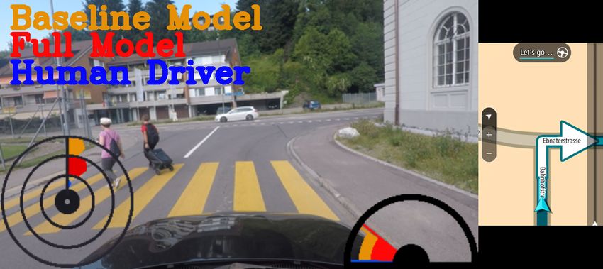
drivers [1, 2, 20]. During the last years, several human-         ing in an end-to-end learning framework, are complemen-
driven cars crashed into autonomous cars. Thankfully, dam-        tary to all methods developed before.
ages were limited. Although there were too few of these              There are also methods dedicated to robust transfer of
cases yet to clearly reveal the underlying causes, experts        driving policies from a synthetic domain to the real world
believe that part of the problem lies with non-human-like         domain [8, 34]. Some other works study how to better eval-
driving behaviours of the autonomous cars. In this work, we       uate the learned driving models [15, 28]. Those works are
take advantage of adversary learning to teach the car about       complementary to our work. Other contributions have cho-
human-like driving. Specifically, a discriminator is trained,     sen the middle ground between traditional pipe-lined meth-
together with our driving model, to distinguish between hu-       ods and the monolithic end-to-end approach. They learn
man driving and our machine driving. The driving model            driving models from compact intermediate representations
is trained to be accurate, comfortable, and at the same time      called affordance indicators such as distance to the front car
to fool the discriminator so that it believes that the driving    and existence of a traffic light [12, 39]. Our engineered fea-
performed by our method was by a human driver. A new              tures from numerical maps can be considered as some sort
evaluation criterion is proposed to score the human-likeness      of affordance indicators. Recently, reinforcement learning
of a driving model.                                               for driving has received increased attention [27,38,42]. The
    This work makes four major contributions: 1) obtaining        trend is especially fueled by the release of multiple driving
numerical map data for real-world driving data, engineering       simulators [17, 41].
map features and showing their effectiveness in a learning           Navigation Maps. Increasing the accuracy and robust-
to drive task; 2) incorporating ride comfort measures into        ness of self-localization on a map [11, 37, 40] and comput-
an end-to-end driving framework; 3) incorporating human-          ing the fastest, most fuel-efficient trajectory from one point
like driving style into an end-to-end driving framework; and      to another through a road network [7, 13, 47, 48, 51] have
4) improving the learning procedure of end-to-end driving         both been popular research fields for many years. By now,
from pointwise predictions to sequence-based predictions.         navigation systems are widely used to aid human drivers or
As a result, we formalize the three major concerns about au-      pedestrians. Yet, their integration for learning driving mod-
tonomous driving into one learning framework. The result          els has not received due attention in the academic commu-
is experimentally demonstrated be a more accurate, com-           nity, mainly due to limited accessibility [23]. We integrate
fortable and human-like driving model.                            industrial standard numerical maps – from HERE Technolo-
                                                                  gies – into the learning of our driving models. We show the
2. Related Work                                                   advantage of using numerical maps and further combine the
Learning Driving Models. Significant progress has been            engineered features of our numerical maps with the visually
made in autonomous driving in the last few years. Classical       rendered navigation routes by [23].
approaches require the recognition of all driving-relevant           Ride Comfort. Cars transport passengers. This has
objects, such as lanes, traffic signs, traffic lights, cars and   led to passenger comfort research for human-driven vehi-
pedestrians, and then perform motion planning, which is           cles [10]. Driver comfort is also considered when devel-
further used for final vehicle control [45]. These type of sys-   oping the control system of human-driven vehicles [3, 50].
tems are sophisticated, represent the current state-of-the-art    Autonomous cars can lead to concerns about how well-
for autonomous driving, but they are hard to maintain and         controlled such a car is [5], motion sickness [18] and ap-
prone to error accumulation over the pipeline.                    parent safety [18]. While research on passenger comfort
    End-to-end mapping methods on the other hand con-             started to receive more attention [18], it is still missing in
struct a direct mapping from the sensory input to the maneu-      current driving models. To address this problem, this work
vers. The idea can be traced back to the 1980s [36]. Other        incorporates passenger comfort measures into learned au-
more recent end-to-end examples include [9, 14, 16, 23, 25,       tonomous driving models.
31, 32, 46]. In [9], the authors trained an end-to-end method        Human-like Driving. A large body of work has stud-
with a collection of front-facing videos. The idea was ex-        ied human driving styles [33, 43]. Statistical approaches
tended later on by using a larger video dataset [46], by          were employed to evaluate human drivers and to suggest
adding side tasks to regularize the training [25,46], by intro-   improvements [35, 49]. This line of research inspired us
ducing directional commands [16] and route planners [23]          to ask whether one can learn and improve machine driv-
to indicate the destination, by using multiple surround-view      ing behaviour such that it is very human-like?. Human-like
cameras to extend the visual field [23], by adding synthe-        driving is hard to quantify. Fortunately, recent advances in
sized off-the-road scenarios [6], and by adding modules to        adversarial learning provide the tools to extract the gist of
predict when the model fails [24]. The main contributions         human-like driving, using it to adjust machine driving so
of this work, namely using numerical map data, incorporat-        that it becomes more human-like. Some work has stud-
ing ride comfort measures, and rendering human-like driv-         ied human-like motion planning of autonomous cars, but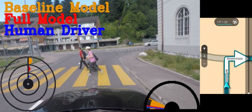
it was constrained to simulated scenarios [1, 2]. The clos-       V = {V |0 ≤ V ≤ 180 for speed and S = {S| − 720 ≤
est work to ours was done by Kuderer et al. [30] where a set      S ≤ 720} for steering angle in our case. Here, kilometer
of manually-crafted features are used to characterize human       per hour (km/h) is the unit of v, and degree (◦ ) the unit of
driving style. Our method learns the features directly from       s. Mt is either a rendered video frame from the TomTom
the data using adversarial neural networks.                       route planner [23], or the engineered features for the numer-
                                                                  ical maps from HERE Technologies (defined in Sec. 3.4), or
3. Approach                                                       the combination of both.
                                                                     In order to keep notations concise, we denote the syn-
   In this section we describe our contributions to improve
                                                                  chronized data (I, M ) as D. Without loss of generality, we
end-to-end driving models: in terms of driving accuracy,
                                                                  assume our training data to consist of a long sequence of
rider comfort, and human-likeness.
                                                                  driving data with T frames in total. Then the basic driv-
3.1. Accurate Driving                                             ing model is to learn the prediction function for the steering
                                                                  angle
    End-to-end driving has allowed the community to de-
                                                                                    ŝt+1 ← fst (D[t−k+1,t] ),               (2)
velop promising driving models based on camera data [16,
23, 46]. The focus has mainly been on perception, not so          and the velocity
much navigation. Thus far, the representations for naviga-
tion are either primitive directional commands in a simu-                            v̂t+1 ← fve (D[t−k+1,t] ),             (3)
lation environment [16, 39] or rendered videos of planned
routes in real-world environments [23].                           with the objective
    We contribute 1) augmenting real-world driving data                      T −1
with numerical map data from HERE Technologies; and 2)
                                                                             X
                                                                                   (|ŝt+1 − st+1 | + λ|v̂t+1 − vt+1 |),    (4)
designing map features believed to be relevant for driving                   t=1
and integrating them into a driving model. To the best of
our knowledge, this work is the first to introduce large-scale    where ŝ and v̂ are predicted values, and s and v are the
numerical map data to driving models in real-world scenar-        ground truth values.
ios. Data acquisition and feature design are discussed in            The learning under Eq. 4 is straightforward and can be
Sec. 3.4, and the usefulness of the map data is validated in      implemented with any standard deep network. This objec-
Sec. 4.                                                           tive, however, assumes the driving decisions at each time
    We adopt the driving model developed in [23]. Given the       step are independent from each other. We believe this is
video I , the map information M, and the vehicle’s location       an over-simplification because driving decisions indeed ex-
L, a deep neural network is trained to predict the steering       hibit strong temporal dependencies within a relatively short
angle s and speed v for a future time step. All data in-          time range. In the following section, we reformulate the ob-
puts are synchronized and sampled at the same sampling            jective by introducing a ride comfort and a human-likeness
rate f , meaning the vehicle makes a driving decision every       score to better model the temporal dependency of driving
1/f seconds. The inputs and outputs are represented in this       actions.
discretized form.
    We use t to indicate the time stamp, such that all data can   3.2. Accurate and Comfortable Driving
be indexed over time. For example, It indicates the current          Multiple concepts relating to driving comfort have been
video frame and vt the vehicle’s current speed. Similarly,        proposed and discussed [10, 18], such as apparent safety,
It−k is the k th previous video frame and st−k is the k th pre-   motion comfort (sickness), level of controllability and re-
vious steering angle. Since predictions need to rely on data      sulting force. While those are all relevant, some are hard to
of previous time steps, we denote the k recent video frames       quantify. We choose to work on motion comfort, which is
by I[t−k+1,t] ≡ hIt−k+1 , ..., It i, and the k recent map rep-    largely influenced by the vehicle’s longitudinal and lateral
resentations by M[t−k+1,t] ≡ hMt−k+1 , ..., Mt i. Our goal        jerk [18, 26, 44]. Due to the short-term predictive nature of
is to train a deep network that predicts desired driving ac-      most end-to-end driving models, substantial jerking is an
tions from the visual observations and the planned route.         inherent problem. Our comfort component aims at reduc-
The learning task can be defined as:                              ing jerk by imposing a temporal smoothness constraint on
                                                                  the longitudinal and lateral oscillations, by minimizing the
       F : (I[t−k+1,t] , M[t−k+1,t] ) → St+1 × Vt+1        (1)
                                                                  second derivative of consecutive steering angle and speed
where St+1 represents the steering angle space and Vt+1 the       predictions.
speed space for future time t + 1. S and V can be defined            Before introducing ride comfort and human-like driving,
at several levels of granularity. We consider the continu-        we reformulate Eq. 4. If the number of consecutive predic-
ous values directly recorded from the car’s CAN bus, where        tions that need to be optimized jointly is denoted by O, then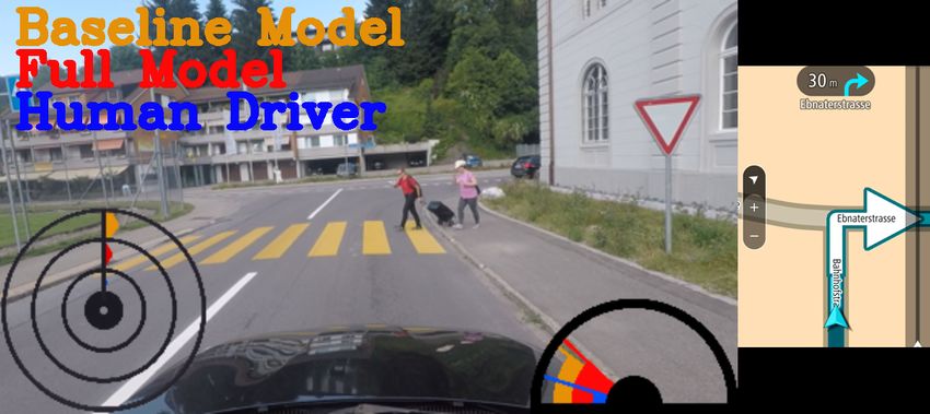
minimizing Eq. 4 is equivalent to minimizing
          −O X
         TX  O
                    (|ŝt+o − st+o | + λ|v̂t+o − vt+o |).        (5)
          t=1 o=1

Then for every O consecutive frames starting at time t, the
loss of driving accuracy will be
                 O
                 X
        Lacc
         t =       (|ŝt+o − st+o | + λ|v̂t+o − vt+o |)          (6)
                 o=1
.
   We can now present the objective function for accurate
                                                                        Figure 1. An illustration of HERE map features used in this work.
and comfortable driving as                                              Please refer to Table 1 for a detailed feature description.
                     −O X
                    TX  O
                                                                           We forward the drivelet at t to G to obtain the driving
                              (Lacc     com
                                t + ζ1 Lt ),                     (7)
                    t=1 o=1
                                                                        actions B̂t . To make autonomous driving more human-like
                                                                        is equivalent to letting the distribution of B̂t approximate
where                                                                   that of Bt . We thus define our loss for human-like driving
                    O−1
                                                                        as an adversarial loss:
                    X     |ŝt+o−1 − 2ŝt+o + ŝt+o+1 |
          Lcom
           t   =                                                                          Lhum = −log(D(B̂t )1 ),                    (9)
                                    (1/f )2                                                t
                    o=2                                   .      (8)
                          |v̂t+o−1 − 2v̂t+o + v̂t+o+1 |                 where D(B̂t )1 is the probability of classifying B̂t as human
                     +λ
                                    (1/f )2                             driving.
                                                                           Putting everything together, our objective for accurate,
ζ1 is a trade-off parameter to balance the two costs. By opti-          comfortable and human-like driving is as follows:
mizing under the objective in Eq. 7, consecutive predictions
are learned and optimized together for accurate and com-                                −O X
                                                                                       TX  O
                                                                                                                     hum
fortable driving.                                                                L=              (Lacc     com
                                                                                                   t + ζ1 Lt ) + ζ2 Lt   .          (10)
                                                                                       t=1 o=1
3.3. Accurate, Comfortable & Human-like Driving
                                                                        ζ2 is a trade-off parameter to control the contributions of the
   If autonomous cars behave differently from human-
                                                                        costs. In keeping with adversarial learning, our training is
driven cars, it is hard for humans to predict their future ac-
                                                                        conducted under the following min-max criterion:
tions. This unpredictability can cause accidents. Also, if
a car behaves more the way its passengers expect, the ride                                   min max L(I, M ).                      (11)
will feel more reassuring. Thus, we argue that it is impor-                                    G     D

tant to design human-like driving algorithms from the very
                                                                        3.4. HERE Navigation
start. Hence, we introduce a human-likeness score. The
higher the value, the closer to human driving. Since it is                 In this section, we first describe how we augment real-
hard to manually define what a human driving style is – as              world driving data, specifically the Drive360 dataset [23]
was done for general comfort measures (Sec. 3.2), we adopt              with map data from HERE Technologies. Then, we present
adversarial learning to model it.                                       our feature extraction to translate obtained map data to fea-
   An adversarial learning method consists of a generator               ture vectors M ’s in order to be used by our driving model.
and discriminator. Our driving model defined in Eq. 4 or                   Obtaining HERE Map Data. Drive360 features 60
in Eq. 7 is the generator G. We now describe the train-                 hours of real-world driving data over 3000 km. We augment
ing objective for the discriminator. For convenience, we                Drive360 with HERE Technologies map data. Drive360
name the short trajectories of O frames used in Sec. 3.2                offers a time stamped GPS trace for each route recorded.
as drivelets. Given the outputs of our driving model for                We use a path-matcher based on a hidden markov model
a drivelet B̂t = (ŝt+1 , ..., ŝt+O , v̂t+1 , ..., v̂t+O ) and its     employing the Viterbi algorithm [19] to calculate the most
corresponding ground truth from the human driver Bt =                   likely path traveled by the vehicle during dataset record-
(st+1 , ..., st+O , vt+1 , ..., vt+O ), the goal is to train a fully-   ing, snapping the GPS trace to the underlying road network.
connected discriminator D using the cross-entropy loss to               This improves our localization accuracy significantly, espe-
classify the two classes (i.e. machine and human).                      cially in urban environments where the GPS signal may be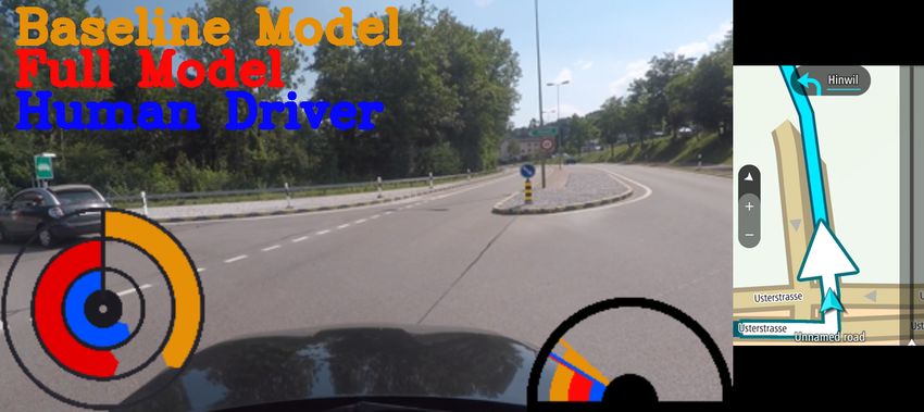
Category and Name                     Range                     Description
 1.a distanceToIntersection            [0m, 250m]                Road-distance to next intersection encounter.
 1.b distanceToTrafficLight            [0m, 250m]                Road-distance to next traffic light encounter.
 1.c distanceToPedestrianCrossing      [0m, 250m]                Road-distance to next pedestrian crossing encounter.
 1.d distanceToYieldSign               [0m, 250m]                Road-distance to next yield sign encounter.
 2.a speedLimit                        [0km/h, 120km/h]          Legal speed limit for road sector.
 2.b freeFlowSpeed                     [0km/h, ∞km/h)            Average driving speed based on underlying road geometry.
 3.a curvature                         [0m−1 , ∞m−1 )            Inverse radius of the approximated road geometry by means
 4.a turnNumber                        [0, ∞)                    Index of road at next intersection to travel (counter-clockwise).
 5.a ourRoadHeading                    [−180◦ , 180◦ )           Relative heading of road that car will take at next intersection.
 5.b otherRoadsHeading                 (−180◦ , 180◦ )           Relative heading of all other roads at next intersection.
                                              ◦   ◦              Relative heading of map matched GPS coordinate in
 6.a - 6.e futureHeadingXm            [−180 , 180 )
                                                                 X ∈ {1, 5, 10, 20, 50} meters.
                                    Table 1. A summary of HERE map data used in this work.
weak and noisy. Through the path matcher we obtain a map           Camera: Our core model consists of a fine-tuned
matched GPS coordinate for each time stamp, which is then          Resnet34 [22] CNN to process sequences of front facing
used to query the HERE Technologies map database to ob-            camera images, followed by two regression networks to pre-
tain the various types of map data.                                dict steering wheel angle and vehicle speed. The architec-
    HERE Technologies has generated an abundant amount             ture is similar to the baseline model from [23]. The model in
of map data. We selected 15 types of data of 6 cate-               this work requires training with a drivelet of O consecutive
gories, as described in Table 1. All features belonging            instances, each having K frames. It means that O + K − 1
to category 1 will be capped at 250m, for example no               frames are used for each camera in each optimization step.
distanceT oT raf f icLight feature is given if the next traf-      This leads to memory issues when using multiple surround-
fic light on route is further than 250m from the current map       view cameras. Thus we choose to proceed with a single
matched position. The features of category 5 specify the           front-facing camera for this work.
relative heading of all roads exiting the next approaching         TomTom: Following [23], a fine-tuned AlexNet [29] is
intersection, with regard to the map matched entry heading,        used to process the visual map representation from the Tom-
see Fig. 1. The features of category 6 specify the relative        Tom Go App.
heading of the planned route a certain distance in advance.        HERE: An LSTM nework with 20 hidden states to process
This relative heading is only calculated with map matched          M [1 − 4] and one fully connected network with three layers
positions. The relative heading is dependent on the road ge-       of size 10 to process M [5 − 6].
ometry and the route taken, see Fig. 1. Using more types           Comfort: No extra network is needed. The loss is com-
of map data constitutes our future work. These augmented           puted according to Eq. 7 and gradients are back propagated
map data will be made publicly available.                          to adjust the driving network.
    Deploying Map Data. Features belonging to categories           Human-like: A fully-connected, three-layer discriminator
1-4 are denoted as M [1 − 4]. At each time step t we sample        network to model human-like driving. The loss is computed
M [1 − 4][t−k,t] with k set to 2s into the past with a step        according to Eq. 9 to adjust the driving network.
size of 0.1s. This gives us a feature vector of 160 elements           This in turn allows us to define a total of five DNN mod-
that we subsequently feed into a small LSTM network. We            els that are composed of combinations of our sub-modules,
found that an LSTM network yields a better performance             see Table 2. Each model is trained on the same 50 hours of
than a fully connected network for these feature categories.       training data of the Drive360 dataset. We employ a discrim-
It is worth noticing that for features belonging to category       inator network D consisting of three fully connected layers
1 we supply the inverse distance capped at 1, effectively al-      each of size 10 to enforce human-like driving by our mod-
lowing for a value range of [0, 1]. Features belonging to          els. D is tasked with classifying maneuvers either as being
categories 5 and 6 are denoted as M [5 − 6]. At each time          human or machine created using a binary cross entropy loss.
t we sample M [5 − 6]t , obtaining a feature vector of size        D is trained using an Adam optimizer with a learning rate
7 that we feed into a small fully connected layer network          of 10−4 . We train with a batch size of 16 for one epoch on
which works well for these two types of features. The engi-        a Titan X GPU. Training for more epochs does not signifi-
neered map features will be publicly released.                     cantly improve convergence, and thus allows us to limit our
                                                                   maximum model training time to around 26 hours. In terms
4. Experiments                                                     of parameter values, we set O to 5, k to 3, λ to 1, ζ1 to 0.1
                                                                   and ζ2 to 1. A larger value for O and k might lead to better
4.1. Implementation Details
                                                                   performance but it requires more computational power and
   The modules of our method are implemented as follows:           GPU memory. Values for the other three parameters are set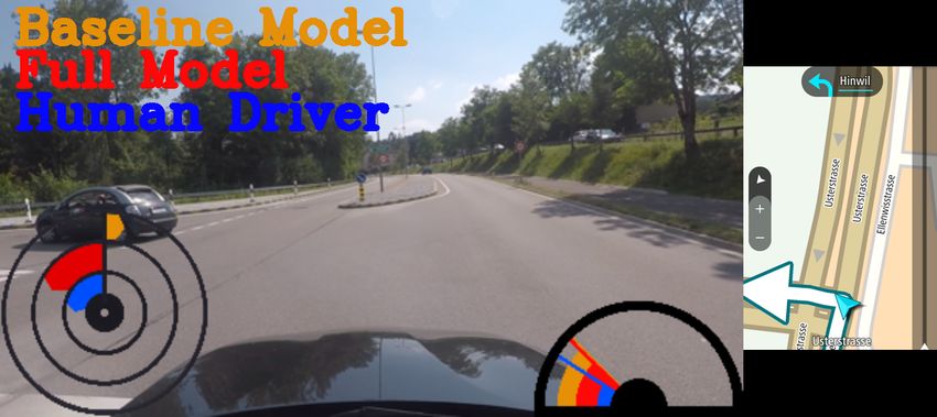
so that the costs are ‘calibrated’ to the same range. The                      (see Table 3). All detailed discussions are given in the fol-
optimal values can be found by cross-validation if needed.                     lowing sections, where we also compare against ablations
                                                                               of our full model (id: 5).
4.2. Evaluation
    A driving model should drive as accurately as possible in                  4.2.1   Driving Accuracy
a wide range of scenarios. As our models are trained via im-
itation learning, we define accuracy as how close the model                    By comparing the performance of M odel1−3 in Table 2,
predictions are to the human ground truth maneuver under                       one can find that driving accuracy improves significantly
the L1 distance metric. We define As as the absolute mean                      when using maps. M odel1 and M odel2 are in fact the same
error in the steering angle prediction and Av as the absolute                  models as used in [23]. The best results are achieved by
mean error in the vehicle speed prediction. Specifically, we                   using HERE numerical features and TomTom visual maps
predict the steering wheel angle St+0.5s and vehicle speed                     together. This implies that the two ways of using map data
Vt+0.5s 0.5s into the future 1 . We use a SmoothL1 loss to                     are to some extent complementary. We reason that the Tom-
jointly train St+0.5s and Vt+0.5s using the Adam Optimizer                     Tom module offers a complete world view, in other words,
with an initial learning rate of 10−4 .                                        an aggregation of all available TomTom map data, rendered
    Evaluation Sets. Our whole test set, denoted by S, con-                    into a video. It is designed to facilitate human driving, but
sisting of around 10 hours of driving, covers a wide range                     it seems that neural networks benefit from having this intu-
of situations including city and countryside driving. While                    itive representation as well. Yet, while the rendered video
one overall number on the whole set is easier to follow, eval-                 is quite effective for representing route information, there
uations on specific scenarios can highlight the strengths and                  is little room left for further improvement towards accurate
weaknesses of driving models at a finer granularity. By en-                    navigation – it is very challenging to reverse engineer all
riching the Drive360 dataset with HERE map data, we can                        exact map information from the rendered videos.
filter our test set S for specific scenarios. We have chosen                       The designed features out of our numerical map data are
three interesting scenarios in this evaluation2 :                              in stark contrast to the rendered video representation. They
                                                                               are accurate and unequivocal. By using numerical map fea-
   • A ⊂ S where the distance to the next traffic light is                     tures, our method M odel3 outperforms [23] which only
     less than 40m or the distance to the next pedestrian                      uses rendered visual maps. It also outperforms [46] which
     crossing is less than 40m and the speed limit is less                     uses no map information. Our engineered HERE map fea-
     than or equal to 50km/h. Translates to approaching a                      tures show marked improvement for challenging driving
     traffic light or pedestrian crossing in the city.                         scenarios. For instance, the error (mse) of steering angle
   • B ⊂ S where the curvature is greater than 0.01 and                        prediction is reduced from 19.69 to 16.83 for scenario ap-
     the speed limit is 80 km/h and the distance to the next                   proaching intersections by using our engineered map fea-
     intersection greater than 100m. Translates to winding                     tures, and the error for speed prediction is reduced from
     road where road radius is less than 100m and no inter-                    4.20 to 3.75 for traffic light or pedestrian crossing. In this
     sections in the vicinity.                                                 work, only fifteen numerical features are hand selected from
   • C ⊂ S where the distance to the next intersection is                      the vast amount of available HERE map features. Logically,
     less than 20m, named approaching an intersection.                         this leaves plenty of room for improving the use of numer-
                                                                               ical map features. This is especially true as the quality of
   Comparison to state-of-the-art. We compare our                              navigation maps keeps improving. For rendered videos, one
method to two start-of-the-art end-to-end driving meth-                        has almost exhausted the ability for further improvement.
ods [46] and [23]. They are trained under the same set-                        Part of our future work will be on incorporating a much
tings as our method is trained. The results are shown at                       larger set of numerical map features.
the top of Table 2. The results show that our method per-
forms better than the two competing methods. It is more
                                                                               4.2.2   Ride Comfort
accurate, more comfortable and behaves more like a human
driver than previous methods. This is due to our numeri-                       By imposing an additional comfort loss, we are able to sig-
cal map features, the sequence-based learning, and two new                     nificantly improve ride comfort by reducing lateral and lon-
learning objectives, namely ride comfort and human-like                        gitudinal oscillations, at a modest loss of driving accuracy.
style. We also compare our method to the classical pro-                        This can be confirmed by comparing the performance of
portional–integral–derivative (PID) controller for improv-                     M odel3 and M odel4 in Table 2. For models that use no
ing ride comfort and show that our method performs better                      map data, we observe a similar trend – significant gains in
   1 Predicting further into the future is possible and our experiments have   comfort at a modest cost in driving accuracy. One direc-
shown a growing degradation in accuracy the further one predicts.              tion to address this issue is to design and learn an adap-
   2 more will be include in the supplementary material.                       tive loss for ride comfort such that it only takes effect when
Model id
Tomtom
Comfort
Camera
Hu-like
S: the whole A: traffic light B: curved C: approaching
HERE evaluation set or pedestrian line mountain road intersections
As ↓ Av ↓ Clat ↓ Clon ↓ H↑ As ↓ Av ↓ H↑ As ↓ Av ↓ H↑ As ↓ Av ↓ H↑
[46] 3 9.81 6.50 2.92 1.46 23.30 14.39 4.97 20.77 10.99 5.12 36.36 21.15 5.41 28.31
[23] 3 3 8.67 4.92 1.60 0.76 27.24 11.94 4.20 24.02 11.10 4.85 36.23 19.69 4.49 33.34
Ours 3 3 3 3 3 7.96 4.79 1.46 0.34 29.31 12.68 3.62 31.56 8.39 3.46 46.64 17.12 4.38 35.68
1 3 10.20 5.84 2.29 0.91 20.20 13.24 4.40 20.85 9.04 4.81 35.86 21.37 4.99 28.34
2 33 8.67 4.92 1.60 0.76 27.24 11.94 4.20 24.02 11.10 4.85 36.23 19.69 4.49 33.34
3 333 8.41 4.81 1.69 0.78 27.72 10.22 3.75 28.72 9.33 4.24 38.62 16.83 4.40 37.21
4 3333 8.81 5.24 1.66 0.41 27.75 11.72 4.51 27.87 12.65 4.99 28.49 18.19 4.85 35.42
5 33333 7.96 4.79 1.46 0.34 29.31 12.68 3.62 31.56 8.39 3.46 46.64 17.12 4.38 35.68
Table 2. The performance of all variants of our method evaluated on the four evaluation sets defined. Driving accuracy is denoted by Av &
As for speed (km/h) and steering angle (degree), comfort measure by Clat & Clon for latitude and longitudinal, and the human-likeliness
score by H (%). ↑ means that higher is better and ↓ the opposite.
Method As ↓ Av ↓ Clat ↓ Clon ↓ H↑ 100
Error for Steering Angle
Relative Error Rate (%)
Yes
[46]+PID 10.72 6.76 1.46 0.34 22.73 80
[23]+PID 8.81 4.85 1.46 0.34 27.56
Left Bend
Yes
Inside
Right Bend
Ours 7.96 4.79 1.46 0.34 29.31 60
Table 3. The performance of [46] and [23] with an additional PID
Approach
30
No
controller evaluated on the full set S. To be read like Table 2 40
50
No
Straight
Depart
None
80
120
20
the driving model is accurate. That is to say, ride comfort
measures are only applied when driving scenarios are easy. 0 Speed Limit (km/h) Traffic Light Cross Walk Road Type Intersection
Otherwise, safety considerations must take prevalence. Us-
100
ing road attributes from our map features can help identify Error for Speed Control
Relative Error Rate (%)
such scenarios. We have also investigated in how far a clas- 80
sical proportional–integral–derivative (PID) controller can
Yes
Yes
Right Bend
60
achieve similar comfort levels to our learned approach. To
Left Bend
No
No
Approach
Straight
this end, we process the network predictions of [46] and
30
Inside
40
Depart
None
50
[23] with tuned (exhaustive grid search for parameters) PID
120
80
controllers such that their comfort score is the same as our 20
learned approach. We report these results in Table 3. This 0 Speed Limit (km/h) Traffic Light Cross Walk Road Type Intersection
shows that reaching similar levels of comfort to our learned Figure 2. Relative Error Rate (%) for five road attributes.
approach with a PID controller comes at the price of de-
graded driving performance and thus our way of including gle and vehicle speed predictions. We observe, again in
comfort in the driving model is preferable. Table 2, that our adversarial learning designed for model-
4.2.3 Human-likeness ing a human-like driving style significantly improves over-
all performance and in particular boosts driving accuracy
A driving style to be human-like is hard to quantify. It is and the human-likeness score, see M odel5 vs M odel4 . In-
also hard to evaluate. In order to evaluate it quanlitatively, terestingly, when a model drives more accurately, due to
we propose a new evaluation criterion – the human-likeness the presence of a navigation component, its human-likeness
score. This score is calculated by clustering human driv- score improves as well. This is evidenced by the perfor-
ing maneuvers (s and v concatenated) from the evaluation mance of M odel1 and M odel3 . This is because the model
set S, over a 0.5s window with a step size of 0.1s, into has a clearer understanding of the driving environment and
75 unique clusters using the Kmeans algorithm. Predicted consequently yields quite comfortable and human-like driv-
model maneuvers are then considered human-like if, for ing already. Overall, the model trained using our human
the same window, they are associated with the same clus- likeness loss, along with the accuracy loss and ride com-
ter as the human maneuver. We chose our window and step fort loss, drives more accurate, more comfortable and more
size to be consistent with our model training. The human- human-like than all previous methods.
likeness score is then defined as the percentage of driving
maneuvers given by an algorithm being associated to the
same cluster as the human driving maneuvers for the same 4.2.4 Error Diagnosis
time window. To this end, and similar to the comfort train-
ing procedure, we generate model driving maneuvers via a It is notoriously difficult to evaluate and understand driving
sequence of five (O = 5) consecutive steering wheel an- model performance solely based on a global quantitative(1)
(2)
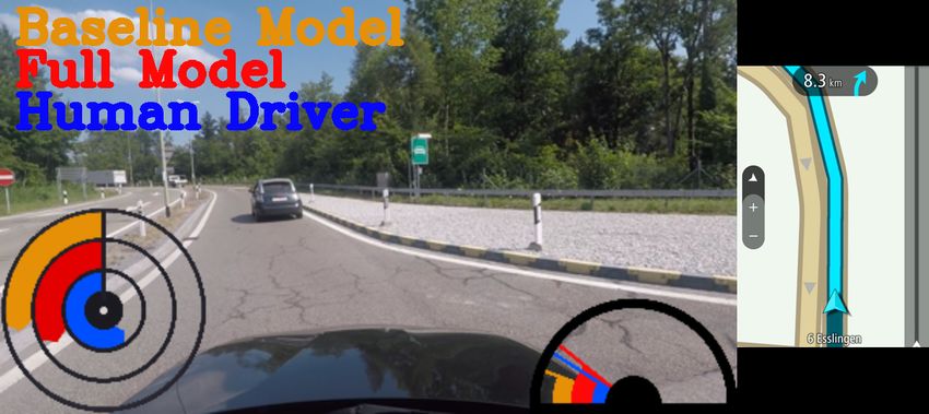
(a) t (b) t +1s (c) t +2s
Figure 3. Qualitative results for future driving action prediction, to compare our full driving model (id: 5) to the baseline of front camera-
only-model (id: 1). Decisions at three time steps over around 2 seconds are shown for two driving scenarios. Better seen on screen.
evaluation. For example, a model with the lowest overall to the human gauge.
test steering error might perform terribly in certain specific Fig. 3 (1) shows the benefit of using maps. M odel1
scenarios. The ability to automatically generate meaningful falsely predicts continuing straight on the road and tries to
evaluation subsets using numerical map features is tremen- compensate for leaving the lane, see (3,b), while M odel5
dously helpful and allows for scenario targeted evaluations accurately predicts the left turn. By using this example, we
as demonstrated in Table 2. In this section, we propose a would like to emphasize again that due attention should be
new evaluation scheme to visualize the correlation of the paid to map data when learning driving models. Fig. 3 (2)
error rate (frequency of making errors) of our final model to shows the benefit of using HERE features. While one may
road attributes. More specifically, five major road attributes claim that M odel5 , being aware of distance to pedestrian
(speed limit, traffic light, cross walk, road type, and inter- crossings, accurately slowed down for the pedestrians in (2,
section) are chosen; for each of them, we define exclusive b) and would, in a real setting not have had an accident,
subsets that collectively complete the test set. We then cal- M odel1 clearly did no such thing. Thus a great benefit of
culate the error-rate for each subset, where, as in [24], error HERE features is that we can automatically filter for these
is defined when steering prediction is off by more than 10 scenarios and evaluate models at a finer granularity. This
deg or speed prediction by more than 5 km/h. For each greatly improves model understanding. Please see the sup-
road attribute, we normalize the error-rates over its subsets. plementary material for a video of animated sequences.
The results are shown in Fig. 2. As can be seen, the model
generally makes more mistakes in more challenging situ- 5. Conclusion
ations. For instance, it makes more mistakes on winding
roads than on straight roads, and makes more mistakes at This paper has extended the objective of autonomous
intersections than along less taxing stretches of road. We driving models from accurate driving to accurate, comfort-
can also see that the model works better on highways than able and human-like driving. The importance of the three
in cities. The results of this error diagnosis provide new in- objectives has been thoroughly discussed, mathematically
sights for the further improvement of existing methods and formulated, and then translated into one neural network
is therefore advisable to include. which is end-to-end trainable. This work made three con-
tributions. First, numerical maps from the leading mapping
company HERE Technologies are employed to augment the
4.2.5 Qualitative Evaluation 3000km real-world driving data of the Drive360 dataset. A
set of driving-relevant features have been extracted to ef-
In Fig. 3 we present two unique driving sequences with fectively use the map information for autonomous driving.
respective model predictions. The steering wheel angle Second, the learning of end-to-end driving models is im-
gauge, on the left, is a direct map of the steering wheel an- proved from pointwise prediction to sequence-based pre-
gle to degrees, whereas the speed gauge, on the right, is diction and a passengers’ comfort measure is included to
from 0km/h to 130km/h. Gauges should be used for relative reduce motion sickness. Finally, adversary learning was in-
model comparison, with our baseline M odel1 prediction in troduced such that the learned driving model behaves more
orange, our most accurate M odel5 prediction in red and the like human drivers. Extensive experiments have shown that
human maneuver in blue. We consider a model to perform our driving model is more accurate, more comfortable and
well when the magnitude of a gauge is identical (or similar) more human-like than previous methods.Acknowledgement This work is funded by Toyota Mo- [14] Y. Chen, J. Wang, J. Li, C. Lu, Z. Luo, H. Xue, and C. Wang.
tor Europe via the research project TRACE-Zurich. We are Lidar-video driving dataset: Learning driving policies effec-
grateful for the support by HERE Technologies for grant- tively. In The IEEE Conference on Computer Vision and Pat-
ing us the access of their map data, without their support tern Recognition (CVPR), June 2018.
this project would not have been possible. We would like [15] F. Codevilla, A. M. Lopez, V. Koltun, and A. Dosovitskiy.
to thank in particular Dr. Harvinder Singh for his insightful On offline evaluation of vision-based driving models. In
ECCV, 2018.
discussions of using HERE map data.
[16] F. Codevilla, M. Müller, A. López, V. Koltun, and A. Doso-
vitskiy. End-to-end driving via conditional imitation learn-
References
ing. 2018.
[1] T. Al-Shihabi and R. R. Mourant. A framework for mod- [17] A. Dosovitskiy, G. Ros, F. Codevilla, A. Lopez, and
eling human-like driving behaviors for autonomous vehicles V. Koltun. CARLA: An open urban driving simulator. In
in driving simulators. In International Conference on Au- Proceedings of the 1st Annual Conference on Robot Learn-
tonomous Agents, 2001. ing, pages 1–16, 2017.
[2] T. Al-Shihabi and R. R. Mourant. Toward more realistic driv- [18] M. Elbanhawi, M. Simic, and R. Jazar. In the passenger
ing behavior models for autonomous vehicles in driving sim- seat: Investigating ride comfort measures in autonomous
ulators. Transportation Research Record, (1):41 – 49, 2003. cars. IEEE Intelligent Transportation Systems Magazine,
[3] N. H. Amer, H. Zamzuri, K. Hudha, and Z. A. Kadir. Mod- 7(3):4–17, 2015.
elling and control strategies in path tracking control for au- [19] G. D. Forney. The viterbi algorithm. Proceedings of the
tonomous ground vehicles: A review of state of the art IEEE, 61(3):268–278, 1973.
and challenges. Journal of Intelligent & Robotic Systems, [20] Y. Gu, Y. Hashimoto, L.-T. Hsu, M. Iryo-Asano, and
86(2):225–254, 2017. S. Kamijo. Human-like motion planning model for driving
[4] R. Attia, R. Orjuela, and M. Basset. Combined longitudinal in signalized intersections. IATSS research, 41(3):129–139,
and lateral control for automated vehicle guidance. Vehicle 2017.
System Dynamics, 52(2):261–279, 2014. [21] L. Han, H. Yashiro, H. T. N. Nejad, Q. H. Do, and S. Mita.
[5] A. Balajee Vasudevan, D. Dai, and L. Van Gool. Object re- Bézier curve based path planning for autonomous vehicle in
ferring in videos with language and human gaze. In CVPR, urban environment. In IEEE Intelligent Vehicles Symposium,
2018. 2010.
[6] M. Bansal, A. Krizhevsky, and A. Ogale. ChauffeurNet: [22] K. He, X. Zhang, S. Ren, and J. Sun. Deep residual learning
Learning to Drive by Imitating the Best and Synthesizing the for image recognition. In 2016 IEEE Conference on Com-
Worst. arXiv e-prints, 2018. puter Vision and Pattern Recognition (CVPR), 2016.
[7] H. Bast, D. Delling, A. V. Goldberg, M. Müller-Hannemann,
[23] S. Hecker, D. Dai, and L. Van Gool. End-to-end learning of
T. Pajor, P. Sanders, D. Wagner, and R. F. Werneck. Route
driving models with surround-view cameras and route plan-
planning in transportation networks. In Algorithm Engineer-
ners. In ECCV, 2018.
ing - Selected Results and Surveys, pages 19–80. 2016.
[24] S. Hecker, D. Dai, and L. Van Gool. Failure prediction for
[8] A. Bewley, J. Rigley, Y. Liu, J. Hawke, R. Shen, V.-D. Lam,
autonomous driving. In IEEE Intelligent Vehicles Symposium
and A. Kendall. Learning to drive from simulation without
(IV), 2018.
real world labels. In ICRA, 2019.
[25] Y. Hou, Z. Ma, C. Liu, and C. C. Loy. Learning to steer by
[9] M. Bojarski, D. Del Testa, D. Dworakowski, B. Firner,
mimicking features from heterogeneous auxiliary networks.
B. Flepp, P. Goyal, L. D. Jackel, M. Monfort, U. Muller,
In AAAI, 2018.
J. Zhang, et al. End to end learning for self-driving cars.
arXiv preprint arXiv:1604.07316, 2016. [26] I. D. Jacobson, L. G. Richards, and A. R. Kuhlthau. Models
[10] J. C. Castellanos and F. Fruett. Embedded system to evalu- of human comfort in vehicle environments. Human factors
ate the passenger comfort in public transportation based on in transport research, 20, 1980.
dynamical vehicle behavior with user’s feedback. Measure- [27] A. Kendall, J. Hawke, D. Janz, P. Mazur, D. Reda, J.-M.
ment, 47:442–451, 2014. Allen, V.-D. Lam, A. Bewley, and A. Shah. Learning to drive
[11] A. Chen, A. Ramanandan, and J. A. Farrell. High-precision in a day. In ICRA, 2019.
lane-level road map building for vehicle navigation. In [28] P. Koopman and M. Wagner. Challenges in autonomous ve-
IEEE/ION Position, Location and Navigation Symposium, hicle testing and validation. SAE Int. J. Trans. Safety, 2016.
2010. [29] A. Krizhevsky, I. Sutskever, and G. E. Hinton. Imagenet
[12] C. Chen, A. Seff, A. Kornhauser, and J. Xiao. Deepdriving: classification with deep convolutional neural networks. In
Learning affordance for direct perception in autonomous Advances in Neural Information Processing Systems. 2012.
driving. In Proceedings of the IEEE International Confer- [30] M. Kuderer, S. Gulati, and W. Burgard. Learning driv-
ence on Computer Vision, pages 2722–2730, 2015. ing styles for autonomous vehicles from demonstration. In
[13] C. Chen, D. Zhang, B. Guo, X. Ma, G. Pan, and Z. Wu. ICRA, 2015.
Tripplanner: Personalized trip planning leveraging heteroge- [31] Y. LeCun, U. Muller, J. Ben, E. Cosatto, and B. Flepp. Off-
neous crowdsourced digital footprints. IEEE Transactions on road obstacle avoidance through end-to-end learning. In
Intelligent Transportation Systems, 16(3):1259–1273, 2015. NIPS, 2005.[32] A. I. Maqueda, A. Loquercio, G. Gallego, N. Garcı́a, and [46] H. Xu, Y. Gao, F. Yu, and T. Darrell. End-to-end learning of
D. Scaramuzza. Event-based vision meets deep learning on driving models from large-scale video datasets. In Computer
steering prediction for self-driving cars. In The IEEE Confer- Vision and Pattern Recognition (CVPR), 2017.
ence on Computer Vision and Pattern Recognition (CVPR), [47] B. Yang, C. Guo, Y. Ma, and C. S. Jensen. Toward personal-
June 2018. ized, context-aware routing. The VLDB Journal, 24(2):297–
[33] G. A. M. Meiring and H. C. Myburgh. A review of intelli- 318, 2015.
gent driving style analysis systems and related artificial in- [48] J. Yuan, Y. Zheng, X. Xie, and G. Sun. Driving with knowl-
telligence algorithms. In Sensors, 2015. edge from the physical world. In ACM SIGKDD Interna-
[34] M. Müller, A. Dosovitskiy, B. Ghanem, and V. Koltun. Driv- tional Conference on Knowledge Discovery and Data Min-
ing policy transfer via modularity and abstraction. In Con- ing, pages 316–324, 2011.
ference on Robot Learning, 2018. [49] H. Zhao, H. Zhou, C. Chen, and J. Chen. Join driving: A
[35] J. Paefgen, F. Kehr, Y. Zhai, and F. Michahelles. Driving be- smart phone-based driving behavior evaluation system. In
havior analysis with smartphones: Insights from a controlled IEEE Global Communications Conference (GLOBECOM),
field study. In International Conference on Mobile and Ubiq- 2013.
uitous Multimedia, 2012. [50] P. Zhao, J. Chen, Y. Song, X. Tao, T. Xu, and T. Mei. De-
[36] D. A. Pomerleau. Nips. chapter ALVINN: An Autonomous sign of a control system for an autonomous vehicle based
Land Vehicle in a Neural Network. 1989. on adaptive-pid. International Journal of Advanced Robotic
Systems, 9(2):44, 2012.
[37] A. Rizaldi and M. Althoff. Formalising traffic rules for ac-
[51] Y.-T. Zheng, S. Yan, Z.-J. Zha, Y. Li, X. Zhou, T.-S. Chua,
countability of autonomous vehicles. In International Con-
and R. Jain. Gpsview: A scenic driving route planner. ACM
ference on Intelligent Transportation Systems, 2015.
Trans. Multimedia Comput. Commun. Appl., 9(1):3:1–3:18,
[38] A. E. Sallab, M. Abdou, E. Perot, and S. Yogamani. Deep 2013.
reinforcement learning framework for autonomous driving.
Electronic Imaging, 2017(19):70–76, 2017.
[39] A. Sauer, N. Savinov, and A. Geiger. Conditional affordance
learning for driving in urban environments. In Conference
on Robot Learning, 2018.
[40] A. Schindler, G. Maier, and F. Janda. Generation of high
precision digital maps using circular arc splines. In IEEE
Intelligent Vehicles Symposium, 2012.
[41] S. Shah, D. Dey, C. Lovett, and A. Kapoor. Airsim: High-
fidelity visual and physical simulation for autonomous vehi-
cles. In Field and Service Robotics conference, 2017.
[42] S. Shalev-Shwartz, S. Shammah, and A. Shashua. Safe,
multi-agent, reinforcement learning for autonomous driving.
arXiv preprint arXiv:1610.03295, 2016.
[43] K. Takeda, J. H. L. Hansen, P. Boyraz, L. Malta, C. Miya-
jima, and H. Abut. International large-scale vehicle corpora
for research on driver behavior on the road. IEEE Trans-
actions on Intelligent Transportation Systems, 12(4):1609–
1623, 2011.
[44] G. M. Turner M1. Motion sickness in public road transport:
the effect of driver, route and vehicle. Ergonomics, (1646-
64), 1999.
[45] C. Urmson, J. Anhalt, H. Bae, J. A. D. Bagnell, C. R. Baker,
R. E. Bittner, T. Brown, M. N. Clark, M. Darms, D. Demitr-
ish, J. M. Dolan, D. Duggins, D. Ferguson, T. Galatali, C. M.
Geyer, M. Gittleman, S. Harbaugh, M. Hebert, T. Howard,
S. Kolski, M. Likhachev, B. Litkouhi, A. Kelly, M. Mc-
Naughton, N. Miller, J. Nickolaou, K. Peterson, B. Pilnick,
R. Rajkumar, P. Rybski, V. Sadekar, B. Salesky, Y.-W. Seo,
S. Singh, J. M. Snider, J. C. Struble, A. T. Stentz, M. Taylor,
W. R. L. Whittaker, Z. Wolkowicki, W. Zhang, and J. Ziglar.
Autonomous driving in urban environments: Boss and the
urban challenge. Journal of Field Robotics Special Issue on
the 2007 DARPA Urban Challenge, Part I, 25(8):425–466,
June 2008.You can also read