Exploring deep learning for air pollutant emission estimation
←
→
Page content transcription
If your browser does not render page correctly, please read the page content below
Geosci. Model Dev., 14, 4641–4654, 2021
https://doi.org/10.5194/gmd-14-4641-2021
© Author(s) 2021. This work is distributed under
the Creative Commons Attribution 4.0 License.

Exploring deep learning for air pollutant emission estimation
Lin Huang1, , Song Liu2,3, , Zeyuan Yang4 , Jia Xing2,3 , Jia Zhang1 , Jiang Bian1 , Siwei Li5,6 , Shovan Kumar Sahu2,3 ,
Shuxiao Wang2,3 , and Tie-Yan Liu1
1 Microsoft Research Lab – Asia, Beijing, China
2 State Key Joint Laboratory of Environmental Simulation and Pollution Control, School of Environment,
Tsinghua University, Beijing, China
3 State Environmental Protection Key Laboratory of Sources and Control of Air Pollution Complex, Beijing, China
4 School of Economics and Management, Tsinghua University, Beijing, China
5 School of Remote Sensing and Information Engineering, Wuhan University, Wuhan, China
6 State Key Laboratory of Information Engineering in Surveying, Mapping and Remote Sensing,

Wuhan University, Wuhan, China
 These authors contributed equally to this work.

Correspondence: Jia Xing (xingjia@tsinghua.edu.cn) and Jia Zhang (zhangjia@microsoft.com)

Received: 16 March 2021 – Discussion started: 29 March 2021
Revised: 25 May 2021 – Accepted: 1 July 2021 – Published: 28 July 2021

Abstract. The inaccuracy of anthropogenic emission inven-       by −1.34 %, −2.65 %, −11.66 %, −19.19 % and 3.51 %, re-
tories on a high-resolution scale due to insufficient basic     spectively, in China for 2015. Such ratios of NOx and PM2.5
data is one of the major reasons for the deviation between      are even higher (∼ 10 %) in regions that suffer from large un-
air quality model and observation results. A bottom-up ap-      certainties in original emissions, such as Northwest China.
proach, which is a typical emission inventory estimation        The updated emission inventory can improve model perfor-
method, requires a lot of human labor and material resources,   mance and make it closer to observations. The mean absolute
whereas a top-down approach focuses on individual pollu-        error for NO2 , SO2 , O3 and PM2.5 concentrations are reduced
tants that can be measured directly as well as relying heav-    significantly (by about 10 %–20 %), indicating the high fea-
ily on traditional numerical modeling. Lately, the deep neu-    sibility of NN-CTM in terms of significantly improving both
ral network approach has achieved rapid development due to      the accuracy of the emission inventory and the performance
its high efficiency and nonlinear expression ability. In this   of the air quality model.
study, we proposed a novel method to model the dual rela-
tionship between an emission inventory and pollution con-
centrations for emission inventory estimation. Specifically,
                                                                1   Introduction
we utilized a neural-network-based comprehensive chemical
transport model (NN-CTM) to explore the complex corre-          Clean air policies have been implemented by the Chinese
lation between emission and air pollution. We further up-       government since 2010 and have been effectively reducing
dated the emission inventory based on back-propagating the      pollutant concentrations, such as sulfur dioxide (SO2 ) and
gradient of the loss function measuring the deviation be-       nitrogen oxides (NOx ) (Zheng et al., 2018). Nevertheless,
tween NN-CTM and observations from surface monitors.            China still faces challenges in addressing O3 and PM2.5 pol-
We first mimicked the CTM model with neural networks            lution. In particular, the level of ozone (O3 ) in China in-
(NNs) and achieved a relatively good representation of the      creased by 1.3 % from 2013 to 2017 (Li, 2019); moreover,
CTM, with similarity reaching 95 %. To reduce the gap be-       concentrations of PM2.5 (particulate matter with an aero-
tween the CTM and observations, the NN model suggests           dynamic diameter less than 2.5 µm) in most Chinese cities
updated emissions of NOx , NH3 , SO2 , volatile organic com-    still far exceed the limits (< 10 µg m−3 ) recommended by
pounds (VOCs) and primary PM2.5 changing, on average,           the World Health Organization (WHO), leading to frequent

Published by Copernicus Publications on behalf of the European Geosciences Union.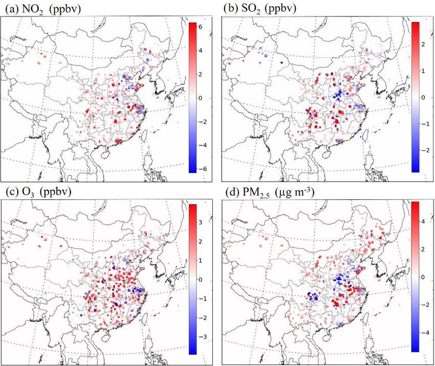
4642                                         L. Huang et al.: Exploring deep learning for air pollutant emission estimation

heavy-pollution events (Guo et al., 2014; Richter et al., 2005;
Vesilind et al., 1988). Such high pollutant concentrations
may substantially affect human health given that air pollu-
tion has being ranked fifth among global risk factors with
respect to mortality (Health Effects Institute, 2019).
   A prerequisite for effectively controlling air pollution lies
in accurate knowledge of the related emission sources. A
well-established emission inventory should summarize the
amount of pollutants emitted into the atmosphere from all
sources in a specific region and during a specific time span
(Health Effects Institute, 2019). A typical bottom-up ap-          Figure 1. Framework of this study.
proach is adopted to develop the emission inventory through
investigation of emission sources in the Air Benefit and
Cost and Attainment Assessment System Emission Inventory           et al., 2019; Wen et al., 2019) have combined recurrent NN
(ABaCAS-EI; Zheng et al., 2019) and the Multi-resolution           (RNN) and convolutional NN (CNN) to capture spatial and
Emission Inventory (MEIC; He, 2012) developed by Ts-               temporal features in air-pollution-related questions, as RNN
inghua University, wherein the activity rate of each source        is skillful with respect to mining temporal patterns from time
is multiplied by an emission factor (Vallero, 2018). Such          series data (Cho et al., 2014; Chung et al., 2014; Hochreiter
technology-oriented bottom-up emission inventories can re-         and Schmidhuber, 1997) and has the ability to handle miss-
flect the types of technology operated in China but are limited    ing values efficiently (Fan et al., 2017), and CNN exhibits po-
with respect to their actual application due to the human la-      tential with respect to leveraging spatial dependencies (e.g.,
bor and material resource requirements, especially in cities       in meteorological prediction; Krizhevsky et al., 2012). Fur-
where thorough investigation is are difficult to support (Xing     thermore, Xing et al. (2020c) applied NN to a response sur-
et al., 2020b). Furthermore, varied assumptions regarding the      face model (RSM), thereby significantly enhancing its com-
activity rate and emission factor from different studies result    putational efficiency and demonstrating the utility of deep
in large uncertainties (Aardenne and Pulles, 2002). There-         learning approaches for capturing the nonlinearity of atmo-
fore, the development of a method for efficient, low-cost and      spheric chemistry and physics. The application of deep learn-
sufficiently accurate grid emission information is being con-      ing improves the efficiency of air quality simulation and can
sidered.                                                           quickly provide data support for the formulation of emission
   The top-down method, as another typical emission inven-         control policies in order to adapt to the dynamic pollution sit-
tory estimation approach, can be used to constrain emission        uation and international circumstances. However, the use of
estimations by combining observation results from surface          deep NN to estimate emission inventories is more complex
monitors and satellite retrievals. Brioude et al. (2012) esti-     than traditional machine learning problems because there are
mated the emissions of anthropogenic CO, NOx and CO2               no precise emission observations that can be used as super-
in the Los Angeles Basin using the FLEXible PARTicle dis-          vision for model training.
persion model (FLEXPART) Lagrangian particle dispersion               To address all of these issues, we proposed a novel method
model based on the top-down method. Recently, Yang et al.          based on dual learning (He et al., 2016), which leverages
(2021) linked the bottom-up China Multi-pollutant Abate-           the primal-dual structure of artificial intelligence (AI) tasks
ment Planning and Long-term benefit Evaluation (China-             to obtain informative feedback and regularization signals,
MAPLE), model with the top-down computable general                 thereby enhancing both the learning and inference process.
equilibrium (CGE) model to evaluate the comprehensive im-          In terms of emission inventory estimation, if we have a pre-
pacts of deep decarbonization pathways (DDPs) in China.            cise relationship between the emission inventory and pollu-
However, most of the previous studies have merely fo-              tion concentrations, we can use the pollution concentrations
cused on individual pollutants that can be measured directly       as a constraint to obtain an accurate emission inventory. In
(Brioude et al., 2012; Xing et al., 2020a; Yang et al., 2021)      particular, we proposed employing a neural-network-based
and have relied on traditional numerical modeling.                 chemical transport model (NN-CTM) with a delicately de-
   On the contrary, neural networks (NNs), as a more effi-         signed architecture, which is efficient and differentiable com-
cient tool, can also model complex nonlinear relations in the      pared with the chemical transport model (CTM). Further-
atmospheric system, thereby converting precursor emissions         more, when a well-trained NN-CTM can accurately reflect
into ambient concentrations. Due to their end-to-end learn-        the direct and indirect physical and chemical reactions be-
ing ability, NNs can automatically extract key features of in-     tween the emission inventory and pollutant concentrations,
put data and capture the behavior of target data; thus, they       the emission inventory can be updated by back-propagating
have recently been widely used in atmospheric science (Fan         the gradient of the error between observed and NN-CTM-
et al., 2017; Tao et al., 2019; Wen et al., 2019; Xing et al.,     predicted pollutant concentrations. Figure 1 shows the frame-
2020a, c). For example, many studies (Fan et al., 2017; Tao        work of this study.

Geosci. Model Dev., 14, 4641–4654, 2021                                             https://doi.org/10.5194/gmd-14-4641-2021
L. Huang et al.: Exploring deep learning for air pollutant emission estimation                                                 4643

Figure 2. The whole process of emission inventory estimation.

   The remainder of this paper is structured as follows: the          g indirectly by leveraging function f . The framework of this
method used for this study is described in Sect. 2; Sect. 3 uses      process is illustrated in Fig. 2. In particular, the whole pro-
the emission inventory estimation over China as an example            cess of emission inventory estimation includes the following
to demonstrate the superiority of our method; in Sect. 4, we          steps:
make a conclusion and discuss some possible future work.
                                                                       1. use the existing emission inventory which is still not ac-
                                                                          curate enough as the initial emission data X̂;
2     Method
                                                                       2. given X̂, calculate the corresponding predicted pollutant
2.1    Main framework                                                     concentration data Ŷ ;
                                                                       3. calculate the loss between the observed values of pollu-
The task of emission inventory estimation can be naturally                tants Y and the predicted pollutant concentrations Ŷ ;
formalized into a typical dual learning framework. Con-
cretely, we denote xt as the data of emission volumes and              4. adjust the estimated emission inventory X̂ by back-
meteorological conditions and yt as the corresponding pollu-              propagating the gradient of the loss based on function
tant concentration at time t. In addition, we denote the map-             f;
ping function from emission to pollutant concentration as f
and that from pollutant concentration to emission as g. As             5. repeat steps 2–4 until achieving sufficient accuracy for
the transformation from emission to pollutant concentration               predicted concentration.
is a continuous process in time, approximately, we have the              Although the CTM system can handle the transition from
following equations:                                                  emission to pollutant concentration, it is not differentiable,
                                                                      which makes it quite hard to update the emission inventory
yt = f (x[(t − k + 1) : t]),                                    (1)   through the back-propagation algorithm in the dual learning
xt = g(y[(t − k + 1) : t]),                                     (2)   framework. In order to establish a differentiable CTM, we
                                                                     propose building a NN-CTM as the system approximation.
where x[i : j ] is defined as  xi , xi+1 , . . ., xj for conve-      More details will be described in the following subsections.
nience, and y[i : j ] represents yi , yi+1 , . . ., yj .
   The formulas above are based on two assumptions:                   2.2   Deep-neural-network-based chemical transition
                                                                            model approximation
    1. The pollutant concentration is only dependent on the
       emission and meteorological conditions in the past k           The pollutant concentration is usually estimated using a
       time steps (e.g., hours or days).                              CTM, which employs the emission inventory as input. In the
    2. There is a bijective relationship between emission and         dual learning framework, this input will, in turn, be updated
       pollutant concentration. This is a necessary prerequisite      based on observed concentrations via the back-propagation
       for the existence of function g.                               algorithm. This requires the CTM to be differentiable. To
                                                                      this end, we propose using deep neural networks to approx-
The first assumption will hold true as long as a sufficiently         imate the CTM system. Concretely, to train this NN-CTM,
large k value is set. The second assumption may not be true           we apply a supervised learning approach that leverages the
unless we introduce more external constraints on the emis-            training data, whose input is the same as that of CTM and
sion inventory, as an information loss exists in the emission-        whose corresponding label is the output of CTM. The whole
to-pollutant concentration process.                                   architecture is shown in Fig. 3.
   In fact, it is quite difficult to obtain the function g di-           The input data for our NN-CTM are similar to that of a
rectly without emission observations as supervision. Hence,           CTM, including emission inventory, meteorology and geo-
we employ a dual learning framework to obtain the function            graphical data. The first two are time dependent, whereas the

https://doi.org/10.5194/gmd-14-4641-2021                                                Geosci. Model Dev., 14, 4641–4654, 2021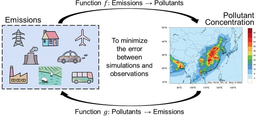
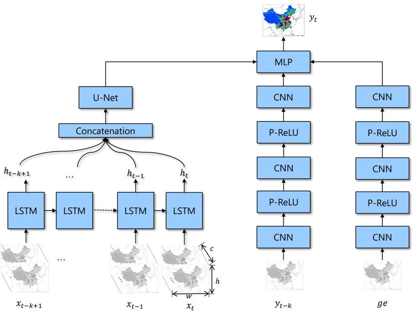
4644                                           L. Huang et al.: Exploring deep learning for air pollutant emission estimation

Figure 3. NN-CTM structure. c represents channel, which consists of the emission inventory and meteorological data. h and w represent the
height and width of input, respectively. ge is geographic information. We employ long short-term memory (LSTM) to capture the temporal
information and U-Net to capture the spatial information. CNN represents the convolution network. P-ReLU (He et al., 2015b) is a nonlinear
activation function. MLP means multiple layers of perceptrons with threshold activation. The model structure is also named LSTM-U-Net.

last one, denoted as ge, is static. In the Eulerian grid-based         The aggregated sequence of hidden states ht−k+1 . . ., ht will
CTM system, for each time step t, the dynamic input data xt            be concatenated and entered into the U-Net block. U-Net is
is a matrix with the following dimensions: w×h×c. The con-             a widely adopted pixel-to-pixel model which can effectively
centration is simulated continuously in a continuous time se-          utilize neighbor information. In U-Net, the stacking of con-
quence. Unlike CTM, the NN-CTM cannot deal with overly                 volution can get neighbor information with a bigger recep-
long data sequences. Thus, we only use the data from past k            tive field (e.g., stacking 5 × 5 convolution and 5 × 5 con-
time steps (i.e, x[t − k + 1 : t]) as input for the pollutant con-     volution can get a 9 × 9 convolution), the nonlinear func-
centration estimation yt . At the same time, we add yt−k as            tion (P-RELU) is employed to improve model fitting with
supplementary input data into the network. The output yt of            nearly zero extra computational cost and little overfitting
NN-CTM is a matrix with the dimensions w × h × l, where l              risk, and the batch normalization and dropout are employed
is the number of pollutant species concerned.                          to enhance the robustness of the model. We calculate that
   The NN-CTM consists of three branches: two CNN                      the receptive field of our model is a 38 × 38 grid. In other
branches for yt−k and ge, and one long short-term mem-                 words, the predicted pollutant concentration is related to its
ory (LSTM; Hochreiter and Schmidhuber, 1997) with U-Net                surrounding 38 × 38 grid’s information, which represents the
(Ronneberger et al., 2015) branch. The CNN branches are                transmission between different grids. Meanwhile, the closer
used to extract features for yt−k and geographical informa-            the distance, the greater the contribution. We employ a two-
tion. We employ a parametric rectified linear unit (P-RELU;            layer U-Net (as shown in Fig. 4) to capture the spatial infor-
He et al., 2015b) as the nonlinear activation function in these        mation between grids.
branches to improve model fitting with nearly zero extra                  In the training process, we take (XCTM , YCTM ) as the
computational cost and little overfitting risk. We adopt the           training dataset, where XCTM denotes the input data of the
architecture of combining LSTM and U-Net based on the un-              CTM system, and YCTM is the corresponding output. As rel-
derstanding of the temporal–spatial relationship in the emis-          ative changes in pollutant concentrations are the metric often
sion inventory. In the temporal dimension, pollutants are the          used by policymakers, we adopt an objective function that
accumulation of historical emissions. In the spatial dimen-            measures the relative loss between NN-CTM-predicted and
sion, adjacent grids will affect each other because of mete-           CTM-simulated pollutant concentrations. We denote the out-
orological and diffusion factors. The LSTM layer is used to
aggregate information from time series data x[t − k + 1 : t].

Geosci. Model Dev., 14, 4641–4654, 2021                                                  https://doi.org/10.5194/gmd-14-4641-2021
L. Huang et al.: Exploring deep learning for air pollutant emission estimation                                                     4645

                                                                         2.3    Emission inventory estimation based on NN-CTM

                                                                         Given a well-trained NN-CTM whose approximation accu-
                                                                         racy is high enough for predicting pollutant concentrations,
                                                                         the emission inventory can be updated based on the error be-
                                                                         tween the observed and NN-CTM-predicted pollutant con-
                                                                         centrations. The observation data will help update the sur-
                                                                         rounding grids’ emission inventory within the receptive field.
                                                                         However, in extreme circumstances, if we have no observa-
                                                                         tion data, our method will not work because we have no more
                                                                         information to adjust the emission inventory. If the obser-
                                                                         vation data are denser, the emission inventory estimation is
                                                                         more accurate because it can consider more observation data.
                                                                            In particular, we make the relationship between emission
Figure 4. U-Net structure (two layers). The model structure yields a     and pollutant concentration more robust by fixing the trained
u-shaped architecture. 3 × 3 conv is a convolution function (Huang       LSTM-U-Net model parameter. By training NN-CTM pa-
et al., 2016). P-ReLU (Huang et al., 2016) is a nonlinear activation     rameter, we then adjust the input emission inventory to mini-
function. Max pooling is a down sample function. Up convolution          mize the loss between the NN-CTM output and the observa-
(Zeiler et al., 2010) is a deconvolution function, which is also named
                                                                         tions. Such loss can be formally defined as follows:
as up sample function.
                                                                                                    N X

                                                                                   ∗
                                                                                              1 X
                                                                                                                    (n)      ∗(n)

                                                                         L ŶNN , Yobs   =                   Mi,j ŷi,j,c − yi,j,c , (5)
put of NN-CTM as ŶNN , and have                                                             N hwl n=1 i,j,c

                             N X
                      1 X             (n)      (n)

L ŶNN , YCTM =                       ŷi,j,c − yi,j,c ,          (3)
                                                                                           ∗

                      N hwl n=1 i,j,c                                           ∂L ŶNN , Yobs
                                                                         ge =                      ,                                 (6)
                                                                                      ∂e

                                                                         where Yobs ∗ represents the observed pollutant concentration
       ∂L ŶNN , YCTM
gw =                       ,                                      (4)    (we use an average value in case of multiple observation sta-
               ∂w                                                        tions in a grid), and Mi,j is a binary indicator variable indi-
                                                                         cating whether or not there is site monitoring equipment in
where N is the number of samples, i ∈ [1, h], j ∈ [1, w] and
                 (n)                                                     grid (i, j ). The emission inventory will be updated by back-
c ∈ [1, l], and yi,j,c represents the concentration of the cth
                                                                         propagating the gradient ge . The stochastic gradient descent
pollutant in the grid with location (i, j ) in the nth sample.
                                                                         (SGD) method (Bottou, 2010) is used as the optimizer.
The parameters of NN-CTM will be updated based on the
                                                                            Meanwhile, aiming at ensuring the reasonableness and ef-
gradients given by gw , and the adaptive moment (Adam) es-
                                                                         fectiveness of the estimated emission inventory, we set two
timation (Kingma and Ba, 2014) is used as the optimizer.
                                                                         constraints. The first is that the update rate of the emission
Model robustness                                                         inventory must be a maximum of 200 % compared with the
                                                                         prior emission for each grid. Biases exist in meteorological
We ensure the robustness of the model from three aspects:                conditions and chemical mechanism, and this determines that
                                                                         we cannot attribute all of the errors to the emission inventory.
  1. model structure – inspired by computer vision tasks, we             If the update ratio is very large, the NN-CTM cannot reflect
     adopt batch normalization (Ioffe and Szegedy, 2015),                the correlation of the unseen data well. Furthermore, the prior
     dropout (Srivastava et al., 2014), L2 regularization                emission is accurate to a certain extent in terms of the spatial
     (Zhang et al., 2016) to improve the generalization and              and temporal dimensions. The second constraint is that the
     robustness;                                                         updated emission inventory must be positive.

  2. early stop – when we train the NN-CTM, we split the
     data into training and validation datasets, and we stop             3     Experiments and the analysis of results
     the model training when the evaluation in the validation
     dataset does not improve within 1000 iterations;                    In this section, we apply our proposed method to emission
                                                                         inventory estimation in China in 2015. In the following, we
  3. data augmentation – during training, we employ the                  will first describe the data and CTM configuration. Subse-
     noise injection, random rescaling, random rotation                  quently, we will show the experimental results in terms of the
     method to avoid the overfitting in training dataset.                accuracy of NN-CTM. We will then conduct further analysis

https://doi.org/10.5194/gmd-14-4641-2021                                                     Geosci. Model Dev., 14, 4641–4654, 2021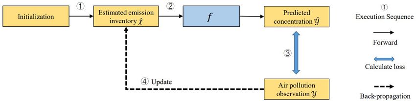
4646                                        L. Huang et al.: Exploring deep learning for air pollutant emission estimation

on the prior emission inventory and our emission inventory       formed in January, April, July and October 2015 to repre-
estimation results.                                              sent winter, spring, summer and autumn, respectively. A 5 d
                                                                 simulation spin-up was performed to minimize the effects of
3.1    Data and CTM configuration                                initial conditions. Pollutant concentrations are analyzed as
                                                                 monthly averages.
The prior high spatial and temporal resolution emission in-
ventory ABaCAS-EI is based on the bottom-up method, in-          3.2   NN-CTM training and evaluation
cluding primary pollutants such as NOx , ammonia (NH3 ),
SO2 , volatile organic compounds (VOCs) and primary              Training parameters
PM2.5 . ABaCAS-EI is a grid-unit-based emission inventory
including sources of power, cement, the steel industry and       The NN-CTM parameters were optimized using the Adam
mobile sources. It also takes technical progress and more        optimizer with a mini-batch size of eight. A learning rate of
stringent emission standards into consideration (Zheng et al.,   0.001 was used. To reduce the risk of over-fitting, we ap-
2019). The prior emission inventory is initially used for NN-    plied weight regularization on all trainable parameters dur-
CTM training and then updated as per the proposed method         ing training and fine-tuning. The NN-CTM was trained for
of dual learning.                                                30 000 epochs.
   Geographical data are a fixed attribute of one grid, like
land type, mountains, depressions or elevation, and they are     Metrics
obtained from the Moderate Resolution Imaging Spectrora-
diometer (MODIS) with a 15 s resolution in this study (Friedl    Model performance was evaluated using the mean absolute
et al., 2002).                                                   error (MAE), which is calculated using the following equa-
   Meteorological conditions are simulated from the Weather      tion:
Research and Forecasting (WRF, version 3.7) model. The                                1 X  (n)              (n)

WRF configuration includes the Morrison microphysics             L ŶNN , YCTM =                    ŷi,j,c − yi,j,c ,           (7)
scheme (Morrison et al., 2009), the RRGM radiation scheme                             N hwl n,i,j,c
(Mlawer et al., 1998, 1997), the Pleim–Xiu land surface
scheme (Pleim and Xiu, 1995; Xiu and Pleim, 2001),               where N , h, w and l are the number of samples, height, width
the Asymmetric Convective Model, version 2 (ACM2)                and the number of observed pollutants in each grid, respec-
planetary boundary layer (PBL) physics scheme (Pleim,            tively. Further, n ∈ [1, N ], i ∈ [1, h], j ∈ [1, w] and c ∈ [1, l].
2007) and the Kain–Fritsch cumulus cloud parameteriza-
tion (Kain, 2004), which matches our previous studies (Ghil      Evaluation
and Malanotte-Rizzoli, 1991; Wikle, 2003). Data assimila-
tion is adopted in WRF simulations based on observation          We examined the performance of NN-CTM to check whether
data for the upper air and surface from the National Cen-        it had learned the relationship between emission and pollu-
ters for Environmental Prediction (NCEP) datasets. The sim-      tant concentration.
ulated temperature, humidity, wind speed and direction show         We trained NN-CTM on the data from the first 22 d in Jan-
good agreement with the observations from the National           uary, April, July and October 2015, and we tested it on the
Climatic Data Center (NCDC, https://www.ncdc.noaa.gov/           remaining successive 8 d of each month. As listed in Table 1,
data-access/land-based-station-data/, last access: 26 Decem-     NN-CTM (with LSTM-U-Net) can reproduce the spatial and
ber 2020) (Ding et al., 2019; Liu et al., 2019; Zhao et al.,     temporal relation well, with a small MAE of 0.27, 0.17,
2013).                                                           1.39 ppbv and 1.46 µg m−3 for NO2 , SO2 , O3 and PM2.5 , re-
   The Community Multiscale Air Quality (CMAQ, ver-              spectively, on average for the 4 months. Results suggest that
sion 5.2) model configured with the AERO6 aerosol mod-           the NN-CTM can reproduce the CTM well within an accept-
ule (Appel et al., 2013) and the Carbon Bond 6 (CB6) gas-        able bias, and thus it can be used for emission adjustment.
phase chemical mechanism (Sarwar et al., 2008) is chosen as      Such a bias (< 4 %) is much smaller than that of the simu-
the representative CTM to simulate pollutant concentrations      lation compared with the observations, which are normally
(Appel et al., 2018; Byun, 1999). Hourly observation data        more than 10 % or even 20 %.
for air pollution (including SO2 , NO2 , O3 and PM2.5 ), which      In order to further verify the superiority of our model
are used to adjust the emission inventory, are obtained from     architecture, we employed ResNet (He et al., 2015a), an-
the China National Environmental Monitoring Centre (http:        other widely adopted deep NN method in image process-
//beijingair.sinaapp.com/, last access: 26 December 2020).       ing. Compared with ResNet, the performance of NN-CTM
   The simulation domain covers mainland China and por-          (with LSTM-U-Net) was superior, with an improved MAE of
tions of surrounding countries with a 27 km × 27 km hori-        0.02, 0.02, 0.10 ppbv and 0.02 µg m−3 for NO2 , SO2 , O3 and
zontal resolution (with h = 182 and w = 232) and 14 verti-       PM2.5 , respectively, on average for the 4 months (as listed in
cal layers from the ground to 100 hPa. Simulations are per-      Table 1).

Geosci. Model Dev., 14, 4641–4654, 2021                                            https://doi.org/10.5194/gmd-14-4641-2021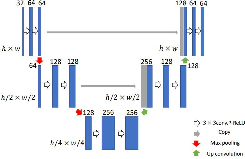
L. Huang et al.: Exploring deep learning for air pollutant emission estimation 4647
Table 1. Evaluation of the NN-CTM simulation in China (mean absolute error between CTM and NN-CTM). LSTM-U-Net is our proposed
method. To compare the model performance, we then select another professional deep neural network method – residual network (ResNet;
He et al., 2015a).
Model NN-CTM (with LSTM-U-Net) NN-CTM (with ResNet)
PM2.5 O3 NO2 SO2 PM2.5 O3 NO2 SO2
Variables (µg m−3 ) (ppbv) (ppbv) (ppbv) (µg m−3 ) (ppbv) (ppbv) (ppbv)
January 1.65 1.39 0.34 0.25 1.65 1.44 0.36 0.26
April 1.74 1.46 0.25 0.16 1.73 1.64 0.26 0.18
July 1.04 1.38 0.23 0.12 1 1.45 0.25 0.13
October 1.43 1.34 0.27 0.16 1.53 1.44 0.29 0.17
Average 1.46 1.39 0.27 0.17 1.48 1.49 0.29 0.19
Error (%) 3.6 3.9 1.9 2.2 3.7 4.3 2.1 2.5
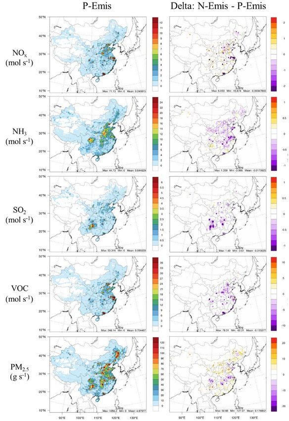
3.3 Emission inventory updating and analysis Table 2. Change ratios of N-Emis compared with P-Emis for the
4 months (given as a percentage).
A well-trained NN-CTM is used to update the emission in-
ventory via back-propagation with the stochastic gradient de- Month Variables
scent (SGD; Bottou, 2010) optimizer with a mini-batch size NOx NH3 SO2 VOCs PM2.5
of two. The learning rate is 0.1. The optimization of emis-
sions is achieved after 10 000 epochs. January 3.72 1.88 −12.38 −25.36 4.64
April −1.49 −2.56 −8.96 −18.27 4.69
For convenience, we denote the emission inventory from
July −11.68 −2.29 −11.42 −12.8 1.8
ABaCAS-EI as prior emissions (P-Emis) and the updated October 3.6 −4.61 −13.32 −19.03 2.4
emission inventory as NN-emissions (N-Emis), which is con-
strained by station observations. Compared with P-Emis, N- Average −1.34 −2.65 −11.66 −19.19 3.51
Emis has adjusted emission rates of NOx , NH3 , SO2 , VOCs
and primary PM2.5 as per the difference between simulated
concentrations and the observed values of pollutants in each
grid, as shown in Fig. 5. Average emission rates of NH3 , pared with SO2 , which may be related to the overestimation
SO2 and VOCs in most grids tend to decrease, whereas those of O3 . The emission of primary PM2.5 tends to increase by
of primary PM2.5 tend to increase except for in the Yangtze less than 5 % for the 4 months.
River Basin, which may be related to the excluded dust emis- Such changes in emissions are based on mathematical al-
sion. Changes in the emission rate of NOx vary a lot by re- gorithms and, thus, cannot be explained by physical and
gion, and such changes are concentrated in urban areas. The chemical processes. The NN method tries to provide a solu-
distribution of N-Emis for each grid is consistent with P- tion to make simulation results of all pollutant species closer
Emis, indicating that the deep learning method in this study to observations by compensating for the errors in the emis-
can identify the distribution of emission sources and focus on sion inventory. For example, concentrations of PM2.5 ob-
the calibration in high-emission areas. tained using P-Emis are generally lower than the observed
Annual anthropogenic emissions in China for NOx , NH3 , level, so the emission of primary PM2.5 will be increased dur-
SO2 , VOCs and primary PM2.5 in P-Emis are 20.44, 10.39, ing the adjustment. SO2 tends to be overestimated using P-
14.40, 23.05 and 7.19 Mt, respectively (Liu et al., 2020), Emis, so the adjustment tends to decrease. However, because
whereas they changed by −1.34 %, −2.65 %, −11.66 %, sulfate is an important component of PM2.5 , the adjustment
−19.19 % and 3.51 %, respectively, in N-Emis. of SO2 will be restricted by the underestimation of PM2.5 .
The sensitivity of change ratios to different seasons varies. Concentrations of O3 obtained using P-Emis are generally
Table 2 lists the change ratios of N-Emis compared with higher than the observed level, so it tends to reduce the emis-
P-Emis for the 4 abovementioned months. As for N-Emis, sions of NOx and VOCs, which are precursors of O3 , during
NOx increases in January and October by about 3.5 %–4.0 %, the adjustment. It is worth noting that the adjustment range of
whereas it decreases by more than 10 % in July. The emis- NOx is much lower than that of VOCs, as only the observed
sion of NH3 increases in January, whereas it decreases in the concentration of NO2 is used as a constraint. Such results are
other 3 months with the highest decrease registered in Octo- consistent with our previous study (Xing et al., 2020a).
ber. The emission of SO2 tends to decrease in all 4 months, In order to further analyze the change in emissions at
with ratios of around 10 %. The emission of VOCs also tends a regional level, we calculated the 4-month average emis-
to decrease but with a larger magnitude of about 20 % com- sions of P-Emis and change ratios of N-Emis for five emis-
https://doi.org/10.5194/gmd-14-4641-2021 Geosci. Model Dev., 14, 4641–4654, 2021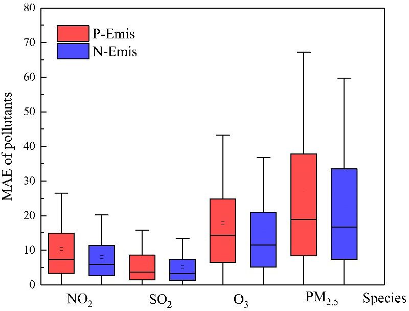
4648                                         L. Huang et al.: Exploring deep learning for air pollutant emission estimation

Figure 5. Emission rates of NOx , NH3 , SO2 , VOCs and primary PM2.5 in P-Emis and their changes in N-Emis.

Geosci. Model Dev., 14, 4641–4654, 2021                                               https://doi.org/10.5194/gmd-14-4641-2021
L. Huang et al.: Exploring deep learning for air pollutant emission estimation 4649
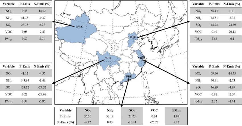
Table 3. Emissions and change ratios in five typical regions for 4 months.
Month Variables Version Regions
BTH YRD PRD SCH NWC
January NOx P-Emis (kt) 68.05 70.56 37.07 43.29 10.26
N-Emis (%) −7.19 6.24 4.55 2.65 8.74
NH3 P-Emis (kt) 28.65 24.42 6.5 24.84 5.52
N-Emis (%) 0.67 0.59 8.3 5.13 8.64
SO2 P-Emis (kt) 90.13 40.16 21.72 150.67 34.06
N-Emis (%) −11.93 −11.38 −13.92 −26.14 −1.5
VOCs P-Emis (Mmol) 0.81 0.99 0.25 0.28 0.05
N-Emis (%) −5.53 −12.73 −37.52 −36.39 2.61
PM2.5 P-Emis (kt) 4.66 2.22 1.14 3.6 0.85
N-Emis (%) 1.27 10.14 15.59 −0.8 9.61
April NOx P-Emis (kt) 52.43 67.17 35.21 39.05 8.72
N-Emis (%) 8.93 −15.05 −5.22 −7.8 14.59
NH3 P-Emis (kt) 85.56 90.34 70.52 192.37 56.06
N-Emis (%) −3.63 −2.6 −0.18 −1.78 −0.43
SO2 P-Emis (kt) 33.93 34.44 20.43 110.74 20.2
N-Emis (%) −28.14 −0.92 −14.17 −22.97 6.77
VOCs P-Emis (Mmol) 0.38 0.85 0.23 0.19 0.05
N-Emis (%) −28.87 13.71 −25.61 −29.06 −2.29
PM2.5 P-Emis (kt) 1.81 1.96 0.94 1.79 0.62
N-Emis (%) −5.12 −3.93 4.34 −8.89 9.54
July NOx P-Emis (kt) 50.51 72.03 36.61 41.35 9.01
N-Emis (%) −10.62 −29.84 −11.46 −11.94 6.86
NH3 P-Emis (kt) 108.78 114.78 89.82 245.68 71.16
N-Emis (%) −5.41 −2.7 −1.1 −0.9 0.08
SO2 P-Emis (kt) 35.65 36.95 21.26 115.74 17.51
N-Emis (%) −38.45 −4.18 −19.26 −19.71 12.71
VOCs P-Emis (Mmol) 0.39 0.92 0.24 0.21 0.05
N-Emis (%) −22.87 23.85 −21.29 −16.47 8.85
PM2.5 P-Emis (kt) 2.34 3.18 1.06 2.27 0.72
N-Emis (%) 0.88 −4.94 4.17 −5.4 6.91
October NOx P-Emis (kt) 54.83 70.11 37.11 40.84 9.96
N-Emis (%) 14.56 −19.99 −9.62 −1.5 25.41
NH3 P-Emis (kt) 50.43 53.4 41.24 110.75 32.28
N-Emis (%) −0.53 −4.52 1.54 −3.79 −2.54
SO2 P-Emis (kt) 35.68 36.08 21.52 116.47 21.74
N-Emis (%) −39.8 −2.73 −19.63 −27.43 −2.39
VOCs P-Emis (Mmol) 0.4 0.89 0.25 0.19 0.06
N-Emis (%) −38.33 27.98 −20.39 −34.42 −16.41
PM2.5 P-Emis (kt) 1.94 1.95 1.15 1.85 1.04
N-Emis (%) 0.26 −4.86 3.8 −13.68 9.32
https://doi.org/10.5194/gmd-14-4641-2021 Geosci. Model Dev., 14, 4641–4654, 20214650 L. Huang et al.: Exploring deep learning for air pollutant emission estimation
Figure 6. Five typical regions of China, the Beijing–Tianjin–Hebei region (denoted as BTH), the Yangtze River Delta (denoted as YRD,
covering Jiangsu, Zhejiang and Shanghai), the Pearl River Delta (denoted as PRD, covering Guangdong), the Sichuan Basin (denoted as
SCH, covering Sichuan and Chongqing) and Northwest China (denoted as NWC, covering Xinjiang), and their monthly average emissions
for 4 months in P-Emis (given in kilotons except for VOCs, which are given in megamoles) and change ratios in N-Emis (given as a
percentage).
sion species in the Beijing–Tianjin–Hebei region (BTH), the
Yangtze River Delta (YRD), the Pearl River Delta (PRD), the
Sichuan Basin (SCH) and Northwest China (NWC), as high-
lighted in Fig. 6. The first four areas were selected because
they are the main population clusters, and NWC was selected
because there are so few observation sites in this area that the
constraints are relatively insufficient.
The adjustment of emission varies greatly by season and
region. Seasonal details are listed in Table 3. The 4-month
average changes in N-Emis in BTH are the highest for SO2
and VOC emissions, reaching about −20 %, whereas those
for NOx , NH3 and primary PM2.5 vary by less than 5 %. In
YRD, NOx and VOC emissions record the highest extent of
changes with −14.73 % for NOx and 12.54 % for VOCs. The
Figure 7. The MAE of NO2 (ppbv), SO2 (ppbv), O3 (ppbv) and
range of changes in other emission species is less than 5 %
PM2.5 (µg m−3 ) concentrations based on P-Emis and N-Emis.
(all decrease). The emission of primary PM2.5 in PRD in-
creases by about 7 %, which is the largest change ratio among
the four urban regions. The emission of NH3 in PRD changes
the least compared with other regions. In SCH, the emissions indicating the large inaccuracy in the emission inventory in
of SO2 and VOCs decrease the most (change ratio) com- NWC.
pared with other emission species (> 20 %). The emission
of primary PM2.5 in SCH, which decreases by 5.95 %, shows 3.4 Accuracy improvements of the CTM simulation for
an opposite trend to that in PRD. As for NWC, emissions pollutants with N-Emis
of NH3 and VOCs show a small decrease (< 5 %), whereas
emissions of NOx and primary PM2.5 have a large percent- We use the CTM to evaluate the accuracy of P-Emis and N-
age increase compared with other regions (10 %), specifically Emis. The configuration of CTM remains constant.
Generally, simulations using P-Emis tend to underestimate
the PM2.5 concentrations and overestimate the O3 concentra-
Geosci. Model Dev., 14, 4641–4654, 2021 https://doi.org/10.5194/gmd-14-4641-2021L. Huang et al.: Exploring deep learning for air pollutant emission estimation 4651 Figure 8. The MAE of NO2 (ppbv), SO2 (ppbv), O3 (ppbv) and PM2.5 (µg m−3 ) concentrations based on P-Emis and N-Emis. tions in China on average for the 4 months, which is con- tend to increase in July and decrease in other months on av- sistent with our previous studies (Ding et al., 2019; Liu et erage in China. Concentrations of NO2 and SO2 tend to de- al., 2019). The underestimation of PM2.5 using P-Emis usu- crease in the 4 abovementioned months, which is consistent ally appears in northern and southeastern China and some- with the direct trend of emission adjustments. times occurs in some provinces of the Yangtze River Basin. We also calculated the average concentrations of four pol- The simulations of O3 using P-Emis are generally overes- lutants in five typical regions to quantify the degree of im- timated at observation sites. Such errors can be narrowed provement in pollutant concentrations after adjusting the when using N-Emis. We calculated the MAE for each sim- emission inventory, as listed in Table 4. Changes in the ulation to compare their performance, considering all obser- NO2 and SO2 concentrations are consistent with adjustments vation sites. After using adjusted emissions (i.e., N-Emis), in emissions but are more sensitive, i.e., a small change the MAE for the NO2 , SO2 , O3 and PM2.5 concentrations (∼ 10 %) in emission results in a larger proportional change reduced significantly from 7.39 to 5.91 ppbv (20.03 %), 3.64 (∼ 20 %) in concentration. The reduced SO2 emission is an to 3.22 ppbv (11.54 %), 14.33 to 11.56 ppbv (19.33 %) and important reason for the improvement in PM2.5 overestima- 18.94 to 16.67 µg m−3 (11.99 %), respectively, on average for tions in the Yangtze River Basin. PM2.5 concentrations in total 612 observation stations (as shown in Fig. 7). Such im- NWC show the highest increase (15 %) compared with other provements prove the advantages of using N-Emis compared regions. As the emission inventory in NWC has great po- with P-Emis. Spatial distributions of the comparison between tential for improvement (subject to production methods and simulations and observations at 612 sites can be found in the acquisition of basic data), the qualitative changes in the Fig. 8. The model performance improved for most stations, PM2.5 concentrations brought about using the NN method while a small number of stations reported reduced perfor- seem meaningful. The increase and decrease in NOx and mance, which shows the link between compound pollutants. VOC emissions directly control the variance in the O3 con- For example, stations with larger deviations between PM2.5 centration. The effect of using N-Emis on the O3 concentra- simulation results and observations tend to have greatly im- tion is not obvious, with a change range of less than 5 % in proved O3 performance and vice versa. typical regions. Although the adjustment ratio of the emis- The difference in monthly simulations using N-Emis and sions of O3 precursors is considerable, the O3 concentration P-Emis as input can be utilized to estimate the seasonal im- does not change by much. This can be linked to the com- pacts of emission changes. Concentrations of O3 and PM2.5 plex relationship of precursor emissions of NOx and VOCs https://doi.org/10.5194/gmd-14-4641-2021 Geosci. Model Dev., 14, 4641–4654, 2021
4652                                           L. Huang et al.: Exploring deep learning for air pollutant emission estimation

Table 4. The 4-month average concentrations of NO2 , SO2 , O3 and PM2.5 in five typical regions using different emission inventories.

                                 Variables           Version                     Regions
                                                                BTH      YRD      PRD       SCH    NWC
                                 NO2 (ppbv)          P-Emis     15.69   13.31      6.25     4.82     0.31
                                                     N-Emis     11.85   10.79      5.29     4.45     0.33
                                 SO2 (ppbv)          P-Emis      6.97     4.32     1.89     4.88     0.26
                                                     N-Emis      5.77     3.95     1.67      3.2     0.37
                                 O3 (ppbv)           P-Emis     34.79   41.63    40.16     41.94   41.42
                                                     N-Emis     35.51    39.7    38.43     40.06   41.47
                                 PM2.5 (µg m−3 )     P-Emis     46.28   44.29     22.6     25.96     2.02
                                                     N-Emis     45.28   41.66    22.08     23.71     2.33

which might not change simultaneously or in the same direc-             such as building a real-time emission monitoring system
tion (e.g., an increase NOx and a decrease in VOCs or vice              based on real-time pollutant observation data.
versa), thereby resulting in only a slight change in the O3
concentration.
                                                                        Code and data availability. The codes for machine learning are
                                                                        available at https://doi.org/10.5281/zenodo.4607127 (Huang et al.,
4   Conclusion and discussion                                           2021), including the demo case for this study with input data
                                                                        from Ding et al. (2016) and the China National Environmen-
                                                                        tal Monitoring Centre (http://beijingair.sinaapp.com/, last access:
In this study, we pioneer the use of machine learning to
                                                                        26 December 2020). CMAQv5.2 is an open-source and pub-
reformulate the problem of emission inventory estimation.
                                                                        licly available model developed by the United States Envi-
It creates a new perspective that the data-driven approach              ronmental Protection Agency, which can be downloaded from
can be applied to automatically improve the quality of the              https://doi.org/10.5281/zenodo.1167892 (US EPA Office of Re-
emission inventory, avoiding manual intervention and empir-             search and Development, 2017; Appel et al., 2018).
ical error. We proposed a differential neural-network-based
chemical transport model (NN-CTM), which achieves a rel-
atively good representation of the CTM. We then employed                Author contributions. LH and SL conceived the research project;
a back-propagation algorithm to update the emission inven-              ZY analyzed the data; JX, JZ, JB, SL, SW and TYL provided valu-
tory based on the deviation between observed and NN-CTM-                able discussions on research and paper organization; LH, SL, ZY,
predicted pollutant concentrations. In terms of method, we              SKS, JX, JZ and JB wrote the paper with contributions from all
proposed a novel emission inventory estimation approach                 co-authors.
based on dual learning that consists of a dual loop: emission-
to-pollution and pollution-to-emission. Results indicate that
our NN-based method with an adjusted emission inventory                 Competing interests. The authors declare that they have no conflict
                                                                        of interest.
performed better than using prior emissions.
   Compared with previous studies, our framework employs
a dual learning mechanism in which the simulated concen-
                                                                        Disclaimer. Publisher’s note: Copernicus Publications remains
trations are compared to ground observations and the gradi-
                                                                        neutral with regard to jurisdictional claims in published maps and
ent is back-propagated to update the emission inventory in              institutional affiliations.
each epoch. Results show that new emissions after the ad-
justment can improve the model performance with respect to
simulating concentrations that are close to observations. The           Acknowledgements. This work was completed on the “Explorer
mean absolute error for the NO2 , SO2 , O3 and PM2.5 con-               100” cluster system of Tsinghua National Laboratory for Informa-
centrations decreased significantly (by 10 % to 20 %). This             tion Science and Technology.
application uses a constant biogenic emission inventory, so
the potential errors in biogenic emissions are also included
in the training of anthropogenic emissions.                             Review statement. This paper was edited by Samuel Remy and re-
   Our method can be naturally extended to other fundamen-              viewed by two anonymous referees.
tal problems, such as CO2 and other greenhouse gas emission
inventory estimations, and has broad application prospects,

Geosci. Model Dev., 14, 4641–4654, 2021                                                    https://doi.org/10.5194/gmd-14-4641-2021
L. Huang et al.: Exploring deep learning for air pollutant emission estimation 4653
Financial support. This work was supported in part by the Na- Sci., IV-4/W2, 15–22, https://doi.org/10.5194/isprs-annals-IV-4-
tional Key R&D Program of China (grant nos. 2016YFC0203306 W2-15-2017, 2017.
and 2017YFC0213005), the National Natural Science Foundation Friedl, M. A., Mciver, D. K., Hodges, J. C. F., Zhang, X. Y.,
of China (grant nos. 41907190 and 51861135102) and the MSRA Muchoney, D., Strahler, A. H., Woodcock, C. E., Gopal, S.,
collaborative research project. Schneider, A., and Cooper, A.: Global land cover mapping from
MODIS: algorithms and early results, Remote Sens. Environ.,
83, 287–302, 2002.
Ghil, M. and Malanotte-Rizzoli, P.: Data Assimilation in Meteorol-
ogy and Oceanography, Adv. Geophys., 33, 141–266, 1991.
References Guo, S., Hu, M., Zamora, M. L., Peng, J., and Zhang, R.: Elucidat-
ing severe urban haze formation in China, P. Natl. Acad. Sci.
Aardenne, J. V. and Pulles, T.: Uncertainty in emission inventories: USA, 111, 17373, https://doi.org/10.1073/pnas.1419604111,
What do we mean and how could we assess it?, Thesis Wagenin- 2014.
gen University, 2002. He, D., Xia, Y., Qin, T., Wang, L., Yu, N., Liu, T.-Y., and Ma, W.-Y.:
Appel, K. W., Pouliot, G. A., Simon, H., Sarwar, G., Pye, H. O. Dual learning for machine translation, Proceedings of the 30th
T., Napelenok, S. L., Akhtar, F., and Roselle, S. J.: Evaluation of International Conference on Neural Information Processing Sys-
dust and trace metal estimates from the Community Multiscale tems, Barcelona, Spain, 820–828, 2016.
Air Quality (CMAQ) model version 5.0, Geosci. Model Dev., 6, He, K.: Multi-resolution Emission Inventory for China (MEIC):
883–899, https://doi.org/10.5194/gmd-6-883-2013, 2013. model framework and 1990–2010 anthropogenic emissions,
Appel, K. W., Napelenok, S., Hogrefe, C., Pouliot, G., Foley, K. American Geophysical Union, Fall Meeting, A32B-05, 2012.
M., Roselle, S. J., Pleim, J. E., Bash, J., Pye, H. O. T., and Heath, He, K., Zhang, X., Ren, S., and Sun, J.: Deep Residual Learning for
N.: Overview and Evaluation of the Community Multiscale Air Image Recognition, arXiv [preprint], arXiv:1512.03385, 2015a.
Quality (CMAQ) Modeling System Version 5.2, in: Air Pollu- He, K., Zhang, X., Ren, S., and Sun, J.: Delving Deep into Recti-
tion Modeling and its Application XXV, edited by: Mensink, C. fiers: Surpassing Human-Level Performance on ImageNet Clas-
and Kallos, G., ITM 2016, Springer Proceedings in Complex- sification, arXiv [preprint], arXiv:1502.01852, 2015b.
ity, Springer, Cham, 69–73, https://doi.org/10.1007/978-3-319- Hochreiter, S. and Schmidhuber, J.: Long Short-Term Memory,
57645-9_11, 2018. Neural Comput., 9, 1735–1780, 1997.
Bottou, L.: Large-Scale Machine Learning with Stochastic Gradient Huang, G., Liu, Z., Laurens, V. D. M., and Weinberger, K. Q.:
Descent, Physica-Verlag HD, 2010. Densely Connected Convolutional Networks, arXiv [preprint],
Brioude, J., Angevine, W. M., Ahmadov, R., Kim, S.-W., Evan, S., arXiv:1608.06993, 2016.
McKeen, S. A., Hsie, E.-Y., Frost, G. J., Neuman, J. A., Pol- Huang, L., Liu, S., Yang, Z., Xing, J., Zhang, J., Bian,
lack, I. B., Peischl, J., Ryerson, T. B., Holloway, J., Brown, J., Li, S., Sahu, S. K., Wang, S., and Liu, T.-Y.: The
S. S., Nowak, J. B., Roberts, J. M., Wofsy, S. C., Santoni, G. Inventory Optimization Code for Exploring Deep Learn-
W., Oda, T., and Trainer, M.: Top-down estimate of surface flux ing in Air Pollutant Emission Estimation Scale, Zenodo,
in the Los Angeles Basin using a mesoscale inverse modeling https://doi.org/10.5281/zenodo.4607127, 2021.
technique: assessing anthropogenic emissions of CO, NOx and Health Effects Institute: State of global air 2019, Health Effects In-
CO2 and their impacts, Atmos. Chem. Phys., 13, 3661–3677, stitute, Boston, 2019.
https://doi.org/10.5194/acp-13-3661-2013, 2013. Ioffe, S. and Szegedy, C.: Batch Normalization: Accelerating Deep
Byun, D.: Science algorithms of the EPA Models-3 community Network Training by Reducing Internal Covariate Shift, arXiv
multiscale air quality (CMAQ) modeling system, U.S. Environ- [preprint], arXiv:1502.03167, 2015.
mental Protection Agency, EPA/600/R-99/030, 1999. Kain, J. S.: The Kain–Fritsch convective parameterization: an up-
Cho, K., Merrienboer, B. V., Bahdanau, D., and Bengio, Y.: On the date, J. Appl. Meteorol., 43, 170–181, 2004.
Properties of Neural Machine Translation: Encoder-Decoder Ap- Kingma, D. and Ba, J.: Adam: A Method for Stochastic Optimiza-
proaches, arXiv [preprint], arXiv:1409.1259, 2014. tion, arXiv [preprint], arXiv:1412.6980, 2014.
Chung, J., Gulcehre, C., Cho, K., and Bengio, Y.: Empirical Evalu- Krizhevsky, A., Sutskever, I., and Hinton, G.: ImageNet Classifi-
ation of Gated Recurrent Neural Networks on Sequence Model- cation with Deep Convolutional Neural Networks, Proceedings
ing, arXiv [preprint], arXiv:1412.3555, 2014. of the 25th International Conference on Neural Information Pro-
Ding, D., Xing, J., Wang, S., Liu, K., and Hao, J.: Esti- cessing Systems, Lake Tahoe, NV, December 2012, 1097–1105,
mated contributions of emissions controls, meteorological fac- 2012.
tors, population growth, and changes in baseline mortality Li, G.: Report on the completion of environmental conditions and
to reductions in ambient PM2.5 and PM2.5 -related mortality environmental protection targets for 2018, The National People’s
in China, 2013–2017, Environ. Health Persp., 127, 067009, Congress, available at: http://wx.h2o-china.com/news/290686.
https://doi.org/10.1289/EHP4157, 2019. html (last access: 26 June 2021), 2019 (in Chinese).
Ding, D., Yun, Z., Jang, C., Lin, C. J., Wang, S., Fu, J., and Jian, Liu, S., Xing, J., Westervelt, D. M., Liu, S., Ding, D., Fiore,
G.: Evaluation of health benefit using BenMAP-CE with an in- A. M., Kinney, P. L., Zhang, Y., He, M. Z., and Zhang, H.:
tegrated scheme of model and monitor data during Guangzhou Role of emission controls in reducing the 2050 climate change
Asian Games, J. Environ., 42, 9–18, 2016. penalty for PM2.5 in China, Sci. Total Environ., 765, 144338,
Fan, J., Li, Q., Hou, J., Feng, X., Karimian, H., and Lin, S.: A Spa- https://doi.org/10.1016/j.scitotenv.2020.144338, 2020.
tiotemporal Prediction Framework for Air Pollution Based on
Deep RNN, ISPRS Ann. Photogramm. Remote Sens. Spatial Inf.
https://doi.org/10.5194/gmd-14-4641-2021 Geosci. Model Dev., 14, 4641–4654, 20214654 L. Huang et al.: Exploring deep learning for air pollutant emission estimation Liu, S., Xing, J., Zhang, H., Ding, D., Zhang, F., Zhao, B., Wikle, C. K.: Atmospheric modeling, data assimi- Sahu, S. K., and Wang, S.: Climate-driven trends of bio- lation, and predictability, Technometrics, 47, 521, genic volatile organic compound emissions and their im- https://doi.org/10.1198/tech.2005.s326, 2003. pacts on summertime ozone and secondary organic aerosol Xing, J., Li, S., Ding, D., Kelly, J. T., and Hao, J.: Data Assimila- in China in the 2050s, Atmos. Environ., 218, 117020, tion of Ambient Concentrations of Multiple Air Pollutants Us- https://doi.org/10.1016/j.atmosenv.2019.117020, 2019. ing an Emission-Concentration Response Modeling Framework, Mlawer, E., Clough, S., and Kato, S.: Shortwave clear-sky model Atmosphere, 11, 1289, https://doi.org/10.3390/atmos11121289, measurement intercomparison using RRTM, in: Proceedings of 2020a. the Eighth ARM Science Team Meeting, 23–27, 1998. Xing, J., Li, S., Jiang, Y., Wang, S., Ding, D., Dong, Z., Zhu, Mlawer, E. J., Taubman, S. J., Brown, P. D., Iacono, M. J., and Y., and Hao, J.: Quantifying the emission changes and associ- Clough, S. A.: Radiative transfer for inhomogeneous atmo- ated air quality impacts during the COVID-19 pandemic on the spheres: RRTM, a validated correlated-k model for the longwave, North China Plain: a response modeling study, Atmos. Chem. J. Geophys. Res.-Atmos., 102, 16663–16682, 1997. Phys., 20, 14347–14359, https://doi.org/10.5194/acp-20-14347- Morrison, H., Thompson, G., and Tatarskii, V.: Impact of cloud mi- 2020, 2020b. crophysics on the development of trailing stratiform precipitation Xing, J., Zheng, S., Ding, D., Kelly, J. T., Wang, S., Li, S., Qin, T., in a simulated squall line: Comparison of one-and two-moment Ma, M., Dong, Z., Jang, C., Zhu, Y., Zheng, H., Ren, L., Liu, schemes, Mon. Weather Rev., 137, 991–1007, 2009. T.-Y., and Hao, J.: Deep Learning for Prediction of the Air Qual- Pleim, J. E.: A combined local and nonlocal closure model for the ity Response to Emission Changes, Environ. Sci. Technol., 54, atmospheric boundary layer. Part I: Model description and test- 8589–8600, 2020c. ing, J. Appl. Meteorol. Climatol., 46, 1383–1395, 2007. Xiu, A. and Pleim, J. E.: Development of a land surface model. Pleim, J. E. and Xiu, A.: Development and testing of a surface flux Part I: Application in a mesoscale meteorological model, J. Appl. and planetary boundary layer model for application in mesoscale Meteorol., 40, 192–209, 2001. models, J. Appl. Meteorol., 34, 16–32, 1995. Yang, X., Pang, J., Teng, F., Gong, R., and Springer, C.: The en- Richter, A., Burrows, J. P., Nüss, H., Granier, C., and Niemeier, U.: vironmental co-benefit and economic impact of China’s low- Increase in nitrogen dioxide over China observed from space, carbon pathways: Evidence from linking bottom-up and top- Nature, 437, 129–132, 2005. down models, Renew. Sustain. Energ. Rev., 136, 110438, Ronneberger, O., Fischer, P., and Brox, T.: U-Net: Convolutional https://doi.org/10.1016/j.rser.2020.110438, 2021. Networks for Biomedical Image Segmentation, arXiv [preprint], Zeiler, M. D., Krishnan, D., Taylor, G. W., and Fergus, R.: Deconvo- arXiv:1505.04597, 2015. lutional networks, 2010 IEEE Computer Society Conference on Sarwar, G., Luecken, D., Yarwood, G., Whitten, G. Z., and Carter, Computer Vision and Pattern Recognition, San Francisco, CA, W. P. L.: Impact of an Updated Carbon Bond Mechanism on Pre- USA, 13–18 June 2010. dictions from the CMAQ Modeling System: Preliminary Assess- Zhang, C., Be Ngio, S., Hardt, M., Recht, B., and Vinyals, O.: ment, J. Appl. Meteorol. Climatol., 47, 3–14, 2008. Understanding deep learning requires rethinking generalization, Srivastava, N., Hinton, G., Krizhevsky, A., Sutskever, I., and arXiv [preprint], arXiv:1611.03530, 2016. Salakhutdinov, R.: Dropout: A Simple Way to Prevent Neural Zhao, B., Wang, S., Wang, J., Fu, J. S., Liu, T., Xu, J., Fu, X., and Networks from Overfitting, J. Mach. Learn. Res., 15, 1929–1958, Hao, J.: Impact of national NOx and SO2 control policies on 2014. particulate matter pollution in China, Atmos. Environ., 77, 453– Tao, Q., Liu, F., Li, Y., and Sidorov, D.: Air Pollution Forecasting 463, 2013. Using a Deep Learning Model Based on 1D Convnets and Bidi- Zheng, B., Tong, D., Li, M., Liu, F., Hong, C., Geng, G., Li, H., Li, rectional GRU, IEEE Access, 7, 76690–76698, 2019. X., Peng, L., Qi, J., Yan, L., Zhang, Y., Zhao, H., Zheng, Y., He, US EPA Office of Research and Development: CMAQ (Version K., and Zhang, Q.: Trends in China’s anthropogenic emissions 5.2), Zenodo, https://doi.org/10.5281/zenodo.1167892, 2017. since 2010 as the consequence of clean air actions, Atmos. Chem. Vallero, D.: Translating Diverse Environmental Data into Reliable Phys., 18, 14095–14111, https://doi.org/10.5194/acp-18-14095- Information, Elsevier Reference Monographs, 25–41, 2017. 2018, 2018. Vesilind, P. A., Peirce, J. J., and Weiner, R. F.: Air Pollution, Zheng, H., Zhao, B., Wang, S., Wang, T., Ding, D., Chang, X., chap. 18, Elsevier Inc., 1988. Liu, K., Xing, J., Dong, Z., and Aunan, K.: Transition in source Wen, C., Liu, S., Yao, X., Peng, L., Li, X., Hu, Y., and Chi, T.: A contributions of PM2.5 exposure and associated premature mor- novel spatiotemporal convolutional long short-term neural net- tality in China during 2005–2015, Environ. Int., 132, 105111, work for air pollution prediction, Sci. Total Environ., 654, 1091– https://doi.org/10.1016/j.envint.2019.105111, 2019. 1099, 2019. Geosci. Model Dev., 14, 4641–4654, 2021 https://doi.org/10.5194/gmd-14-4641-2021
You can also read