Fast Keypoint Recognition using Random Ferns - CVLab EPFL
←
→
Page content transcription
If your browser does not render page correctly, please read the page content below
Fast Keypoint Recognition using Random Ferns

          Mustafa Özuysal, Michael Calonder, Vincent Lepetit and Pascal Fua
                     Ecole Polytechnique Fédérale de Lausanne (EPFL)
                           Computer Vision Laboratory, I&C Faculty
                                   CH-1015 Lausanne, Switzerland
                                     {Mustafa.Oezuysal,
     Michael.Calonder,Vincent.Lepetit,Pascal.Fua}@epfl.ch
                                    http://cvlab.epfl.ch

                                              Abstract

    While feature point recognition is a key component of modern approaches to object detection,
existing approaches require computationally expensive patch preprocessing to handle perspective distor-
tion. In this paper, we show that formulating the problem in a Naive Bayesian classification framework
makes such preprocessing unnecessary and produces an algorithm that is simple, efficient, and robust.
Furthermore, it scales well as number of classes grows.
    To recognize the patches surrounding keypoints, our classifier uses hundreds of simple binary
features and models class posterior probabilities. We make the problem computationally tractable by
assuming independence between arbitrary sets of features. Even though this is not strictly true, we
demonstrate that our classifier nevertheless performs remarkably well on image datasets containing very
significant perspective changes.

                                            Index Terms

    Image processing and computer vision, object recognition, tracking, image registration, feature
matching, naive bayesian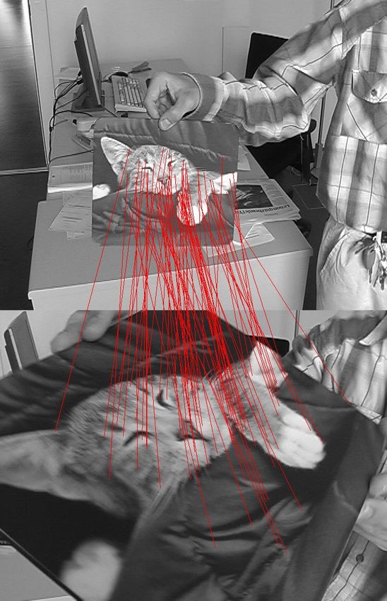
1

                                                     I. I NTRODUCTION

      Identifying textured patches surrounding keypoints across images acquired under widely vary-
ing poses and lightning conditions is at the heart of many Computer Vision algorithms. The
resulting correspondences can be used to register different views of the same scene, extract 3D
shape information, or track objects across video frames. Correspondences also play a major role
in object category recognition and image retrieval applications.
      In all these cases, since patch recognition is one of the first and most critical stages in the
algorithmic pipeline, reliability and speed are key to the overall success and practicality of
the corresponding applications. Achieving both is difficult because surface appearance around a
keypoint can vary drastically depending on how the images were captured. The standard approach
to addressing this problem is to build affine-invariant descriptors of local image patches and to
compare them across images. This usually involves fine scale selection, rotation correction, and
intensity normalization [23], [22]. It results in a high computational overhead and often requires
handcrafting the descriptors to achieve insensitivity to specific kinds of distortion.
      In earlier work [20], we have shown that casting the matching problem as a more generic
classification problem leads to solutions that are much less computationally demanding. This
approach relies on an offline training phase during which multiple views of the patches to be
matched are used to train randomized trees [2] to recognize them based on a few pairwise
intensity comparisons. This yields both fast run-time performance and robustness to viewpoint
and lighting changes.
      Here we show that the trees can be profitably replaced by non-hierarchical structures that we
refer to as ferns to classify the patches. Each one consists of a small set of binary tests and
returns the probability that a patch belongs to any one of the classes that have been learned
during training. These responses are then combined in a Naive Bayesian way. As before, we
train our classifier by synthesizing many views of the keypoints extracted from a training image
as they would appear under different perspective or scale. The ferns are just as reliable as the
randomized trees but much faster and simpler to implement. The code that implements patch
evaluation can be written in ten lines of C++ code, which highlights the simplicity of the resulting
implementation and the complete software package is available [29] 1 .

  1
      We make the code available under http://cvlab.epfl.ch/software

November 7, 2008                                                                               DRAFT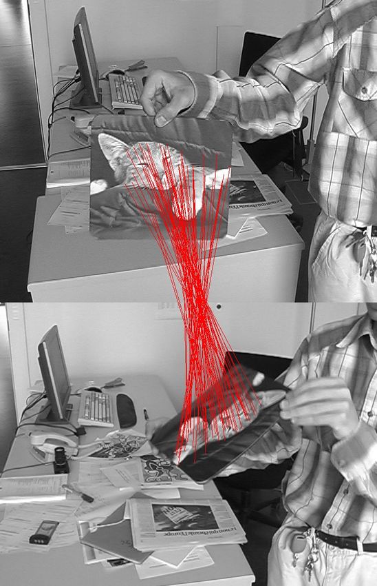
2

   The binary tests we use as classifier features are picked completely at random, which puts
our approach firmly in the camp of techniques that rely on randomization to achieve good
performance [1]. We will show that this is particularly effective for applications such as real-
time 3D object detection and Simultaneous Localization and Mapping (SLAM) that require scale
and perspective invariance, involve a very large number of classes, but can tolerate significant
error rates since we use robust statistical methods to exploit the information provided by the
correspondences. Furthermore, our approach is particularly easy to implement, does not overfit,
does not require ad hoc patch normalization, and allows fast and incremental training.

                                         II. R ELATED WORK

   Due to its robustness to partial occlusions and computational efficiency, recognition of image
patches extracted around detected keypoints is crucial for many vision problems. As a result,
two main classes of approaches have been developed to achieve robustness to perspective and
lighting changes.
   The first family relies on local descriptors designed to be invariant, or at least robust, to specific
classes of deformations [30], [22]. These approaches usually rely on the fine scale and rotation
estimates provided by the keypoint detector. Among these, the SIFT vector [22], computed from
local histograms of gradients, has been shown to work remarkably well and we will use it as a
benchmark for our own approach. It has also been shown that keypoints can be used as visual
words [31] for fast image retrieval in very large image databases [27]. Keypoints are labeled
by hierarchical k-means [5] clustering based on their SIFT descriptors. This makes it possible
to use very many visual words. However, performance is measured in terms of the number of
correctly retrieved documents rather than the number of correctly classified keypoints, which is
the important criterion for applications such as pose estimation or SLAM.
   A second class relies on statistical learning techniques to compute a probabilistic model of
the patch. The one-shot approach of [13] uses PCA and Gaussian Mixture Models but does not
account for perspective distortion. Since the set of possible patches around an image feature
under changing perspective and lightning conditions can be seen as a class, we showed that this
problem can be overcome by training a set of Randomized Trees [2] to recognize feature points
independently of pose [20]. This is done using a database of patches obtained by warping those
found in a training image by randomly chosen homographies.

November 7, 2008                                                                                   DRAFT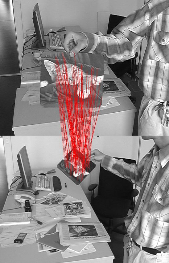
3

                                                                                   # of Inlier Comparison
                                                              300

                                                              250

                                                              200
                                      # of inliers for SIFT

                                                              150

                                                              100

                                                               50

                                                                0
                                                                    0   50   100              150            200   250   300
                                                                                    # of inliers for Ferns

Fig. 1. Matching a mouse pad in a 1074-frame sequence against a reference image. The reference image appears at the top and
the input image from the video sequence at the bottom. : Top row. Matches obtained using ferns in a few frames. Middle row.
Matches obtained using SIFT in the same frames. Bottom row. Scatter plot showing the number of inliers for each frame. The
values on the x and y axes give the number of inliers for Ferns and SIFT, respectively. Most of the time, the Ferns match at
least as many points as SIFT and often even more, as can be seen from the fact that most of the points lay below the diagonal.

November 7, 2008                                                                                                               DRAFT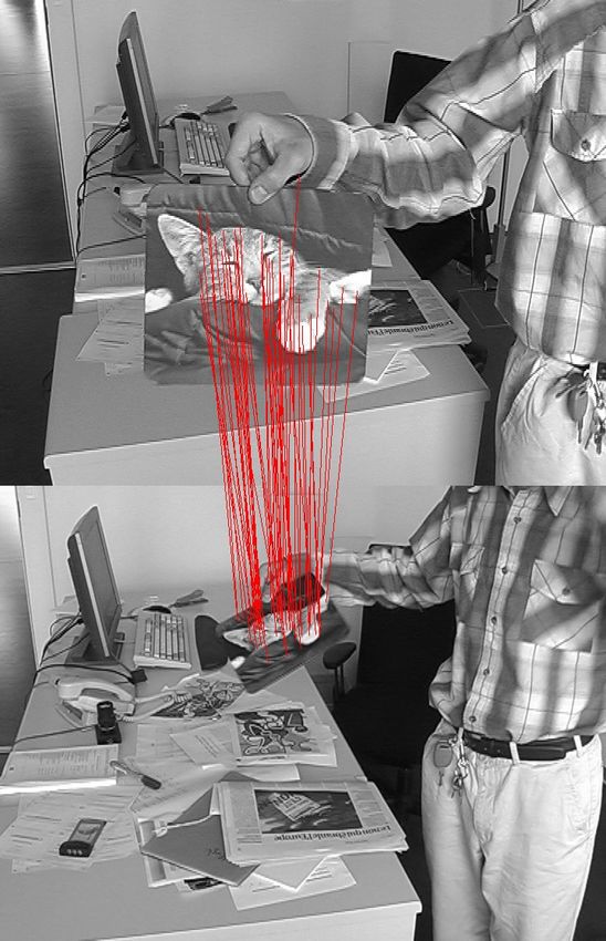
4

   This approach is fast and effective to achieve the kind of object detection depicted by Figure 1.
Note that unlike in traditional classification problems, a close-to-perfect method is not required,
because the output of the classifier can be filtered by a robust estimator. However the classifier
should be able to handle many classes—typically more than 400— simultaneously without
compromising performance or speed. For this purpose, we will demonstrate that the approach
we propose is even faster than the trees [20], more scalable, and just as reliable.
   Local Binary Patterns [28], also rely on binary feature statistics by describing the underlying
texture in terms of histograms of binary features over all pixels of a target region. While such
a description is appropriate for texture classification, it is not directly suitable for keypoint
characterization since histograms are built in this way, it will lose the spatial information between
the features. By contrast, we compute the statistics of the binary features over example patches
seen from different viewpoints and use independence assumptions between groups of features,
hence using many more features centered on the keypoint location, to improve the recognition
rate.
   The Real-Time SLAM method of [35] also extends the RT’s into lists of features (very similar
to our Ferns), but the full posterior distribution over binary features are replaced by a single bit.
This design choice is aimed at significantly reducing the memory requirements while correctly
matching the sparse set of visible landmarks at a time. For maximum performance, we model
the full joint probability of the features. Memory requirements can be tackled by using fixed
point representations that require fewer bits than the standard floating point representation.
   Trees and Ferns have recently been used for the image classification task, as a replacement for
a multi-way Support Vector Machine [6]. The binary features are computed on shape and texture
descriptors, hence gaining invariance to local deformations. The distributions are computed over
different instances of the same class, but unlike our approach the posteriors from different Trees
and Ferns are combined by averaging in both cases. The results match our own observations
that using either Fern or Tree structures leads to similar classification performance.

                   III. A S EMI -NAIVE BAYESIAN A PPROACH   TO   PATCH R ECOGNITION

   As discussed in Section II, image patches can be recognized on the basis of very simple
and randomly chosen binary tests that are grouped into decision trees and recursively partition
the space of all possible patches [20]. In essence, we treat the set of possible appearances of

November 7, 2008                                                                               DRAFT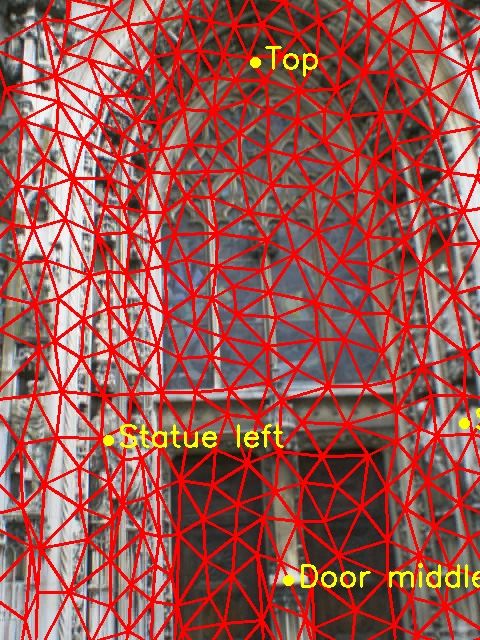
5
a keypoint as classes and the Randomized Trees (RTs) embody a probability distribution over
these classes. In practice, no single tree is discriminative enough when there are many classes.
However, using a number of trees and averaging their votes yields good results because each
one partitions the feature space in a different way.
In this section, we will argue that, when the tests are chosen randomly, the power of the
approach derives not from the tree structure itself but from the fact that combining groups
of binary tests allows improved classification rates. Therefore, replacing the trees by our non-
hierarchical ferns and pooling their answers in a Naive Bayesian manner yields better results
and scalability in terms of number of classes. As a result, we can combine many more features,
which is key to improved recognition rates.
We first show that our non-hierarchical fern structures fit nicely into a Naive Bayesian frame-
work and then explain the training protocol which is similar to the one used for RTs.
A. Formulation of Feature Combination
As discussed in Section II we treat the set of all possible appearances of the image patch
surrounding a keypoint as a class. Therefore, given the patch surrounding a keypoint detected
in an image, our task is to assign it to the most likely class. Let ci , i = 1, . . . , H be the set of
classes and let fj , j = 1, . . . , N be the set of binary features that will be calculated over the
patch we are trying to classify. Formally, we are looking for
cˆi = argmax P (C = ci | f1 , f2 , . . . , fN ) ,
ci
where C is a random variable that represents the class. Bayes’ Formula yields
P (f1 , f2 , . . . , fN | C = ci )P (C = ci )
P (C = ci | f1 , f2 , . . . , fN ) = .
P (f1 , f2 , . . . , fN )
Assuming a uniform prior P (C), since the denominator is simply a scaling factor that it is
independent from the class, our problem reduces to finding
cˆi = argmax P (f1 , f2 , . . . , fN | C = ci ) . (1)
ci
In our implementation, the value of each binary feature fj only depends on the intensities of
two pixel locations dj,1 and dj,2 of the image patch. We therefore write
1 if I(d ) < I(d )
j,1 j,2
fj = ,
0 otherwise
November 7, 2008 DRAFT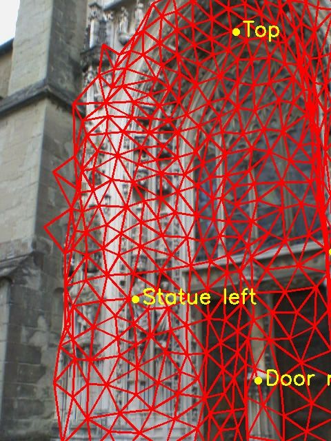
6

where I represents the image patch. Since these features are very simple, we require many
(N ≈ 300) for accurate classification. Therefore a complete representation of the joint probability
in Eq. (1) is not feasible since it would require estimating and storing 2N entries for each class.
One way to compress the representation is to assume independence between features. An extreme
version is to assume complete independence, that is,
                                                                 N
                                                                 Y
                          P (f1, f2 , . . . , fN | C = ci ) =          P (fj | C = ci ) .
                                                                 j=1

   However this completely ignores the correlation between features. To make the problem
tractable while accounting for these dependencies, a good compromise is to partition our features
                                N
into M groups of size S =       M
                                  .   These groups are what we define as Ferns and we compute the
joint probability for features in each Fern. The conditional probability becomes
                                                                 M
                                                                 Y
                          P (f1 , f2 , . . . , fN | C = ci ) =         P (Fk | C = ci ) ,                (2)
                                                                 k=1

where Fk = {fσ(k,1) , fσ(k,2) , . . . , fσ(k,S) }, k = 1, . . . , M represents the k th fern and σ(k, j) is a
random permutation function with range 1, . . . , N. Hence, we follow a Semi-Naive Bayesian [36]
approach by modelling only some of the dependencies between features. The viability of such
an approach has been shown by [18] in the context of image retrieval applications.
   This formulation yields a tractable problem that involves M ×2S parameters, with M between
30-50. In practice, as will be shown in Section IV, S = 11 yields good results. M ×2S is therefore
in the order of 80000, which is much smaller than 2N with N ≈ 450 that the full joint probability
representation would require. Our formulation is also flexible since performance/memory trade-
offs can be made by changing the number of Ferns and their sizes.
   Note that we use randomization in feature selection but also in grouping. An alternative
approach would involve selecting feature groups to be as independent from each other as possible.
This is routinely done by Semi-Naive Bayesian classifiers based on a criteria such as the mutual
information between features [8]. However, in practice, we have not found this to be necessary
to achieve good performance. We have therefore chosen not to use such a strategy to preserve
the simplicity and efficiency of our training scheme and to allow for incremental training.

November 7, 2008                                                                                      DRAFT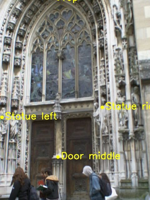
7

B. Training

   We assume that at least one image of the object to be detected is available for training. We
call any such image as a model image. Training starts by selecting a subset of the keypoints
detected on these model images. This is done by deforming the images many times, applying
the keypoint detector, and keeping track of the number of times the same keypoint is detected.
The keypoints that are found most often are assumed to be the most stable and retained. These
stable keypoints are assigned a unique class number.
   The training set for each class is formed by generating thousands of sample images with
randomly picked affine deformations by sampling the deformation parameters from a uniform
distribution, adding Gaussian noise to each sample image, and smoothing with a Gaussian filter
of size 7 ×7. This increases the robustness of the resulting classifier to run-time noise, especially
when there are features that compare two pixels on a uniform area.
   The training phase estimates the class conditional probabilities P (Fm | C = ci ) for each Fern
Fm and class ci , as described in Eq. 2. For each Fern Fm we write these terms as:

                                  pk,ci = P (Fm = k | C = ci ) ,                                 (3)

where we simplify our notations by considering Fm to be equal to k if the base 2 number formed
by the binary features of Fm taken in sequence is equal to k. With this convention, Ferns can
take K = 2S values and, for each one, we need to estimate the pk,ci , k = 1, 2, . . . , K under the
constraint
                                           K
                                           X
                                                 pk,ci = 1.
                                           k=1

The simplest approach would be to assign the maximum likelihood estimate to these parameters
from the training samples. For parameter pk,ci it is
                                                     Nk,ci
                                           pk,ci =         ,
                                                     Nci
where Nk,ci is the number of training samples of class ci that evaluates to Fern value k and Nci
is the total number of samples for class ci . These parameters can therefore be estimated for each
Fern independently.
   In practice however, this simple scheme yields poor results because if no training sample for
class ci evaluates to k, which can easily happen when the number of samples is not infinitely
large, both Nk,ci and pk,ci will be zero. Since we multiply the pk,cj for all Ferns, it implies

November 7, 2008                                                                               DRAFT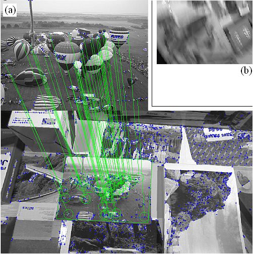
8

                                                                            Effect of Prior on Recognition Rate
                                                  100

                                                   95

                                                   90

                               Recognition Rate
                                                   85

                                                   80

                                                   75

                                                           City
                                                           Flowers
                                                           Museum
                                                   70
                                                      −6     −5        −4        −3          −2           −1       0    1    2
                                                    10     10         10      10           10           10        10   10   10
                                                                                            N
                                                                                             r

Fig. 2.   Recognition rate as a function of log(Nr ) using the three test images of Section IV. The recognition rate remains
relatively constant for 0.001 < Nr < 2. For Nr < 0.001 it begins a slow decline, which ends in a sudden drop to about 50%
when Nr = 0. The rate also drops when Nr is too large because too strong a prior decreases the effect of the actual training
data, which is around 10000 samples for this experiment.

that, if the Fern evaluates to k, the corresponding patch can never be associated to class ci , no
matter the response of the other Ferns. This makes the Ferns far too selective because the fact
that pk,ci = 0 may simply be an artifact of the necessarily limited size of the training set. To
overcome this problem we take pk,ci to be
                                                                                    Nk,ci + Nr
                                                                     pk,ci =                    ,
                                                                                   Nci + K × Nr
where Nr represents a regularization term, which behaves as a uniform Dirichlet prior [4] over
feature values. If a sample with a specific Fern value is not encountered during training, this
scheme will still assign a non-zero value to the corresponding probability. As illustrated by
Figure 2, we have found our estimator to be insensitive to the exact value of Nr and we use
Nr = 1 in all our experiments. However, having Nr be strictly greater than zero is essential.
This tallies with the observation that combining classifiers in a Naive Bayesian fashion can be
unreliable if improperly done [19].
   In effect, our training scheme marginalizes over the pose space since the class conditional
probabilities P (Fm | C = ci ) depend on the camera poses relative to the object. By densely
sampling the pose space and summing over all samples, we marginalize over these pose param-

November 7, 2008                                                                                                                 DRAFT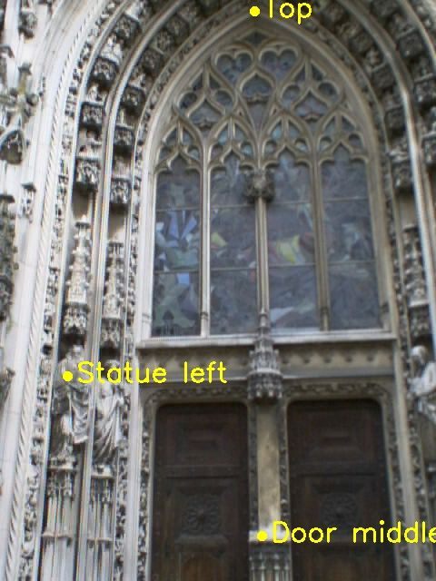
9

                             f0                                            f0                                     f0

                   f1                  f2                       f1                    f1                          f1

            f3          f4        f5         f6            f2         f2        f2         f2                     f2

Fig. 3.   Ferns vs Trees. A tree can be transformed into a Fern by performing the following steps. First, we constrain the tree
to systematically perform the same test across any given hierarchy level, which results in the same feature being evaluated
independently of the path taken to get to a particular node. Second, we do away with the hiearchical structure and simply store
the feature values at each level. This means applying a sequence of tests to the patch, which is what Ferns do.

                                       (a)                                                      (b)

Fig. 4.   The feature spaces of Trees and Ferns. Although the space of tree features seems much higher dimensional, it is not
because only a subset of features can be evaluated. (a) For the simple tree on the left only the 4 combination of feature values
denoted by green circles are possible. (b) The even simpler Fern on the left also yields 4 possible combinations of feature values
but a much simpler structure. As shown below, this simplicity does not entail any performance loss.

eters. Hence at run-time, the statistics can be used in a pose independent manner, which is key
to real-time performance. Furthermore, the training algorithm itself is very efficient since it only
requires storing the Nk,ci counts for each fern while discarding the training samples immediately
after use, which means that we can use arbitrarily many if need be.

                                  IV. C OMPARISON         WITH     R ANDOMIZED T REES

   As shown in Figures 3 and 4, Ferns can be considered as simplified trees. Whether or not this
simplification degrades their classification performance hinges on whether our randomly chosen

November 7, 2008                                                                                                          DRAFT
10
Fig. 5. The recognition rate experiments are performed on three images that show different texture and structures. Image size
is 640 × 480 pixels.
binary features are still appropriate in this context. In this section, we will show that they are
indeed. In fact, because our Naive Bayesian scheme outperforms the averaging of posteriors used
to combine the output of the decision trees [20], the Ferns are both simpler and more powerful.
To compare RTs and Ferns, we experimented with the three images of Figure 5. We warp
each image by repeatedly applying random affine deformations and detect Harris corners in the
deformed images. We then select the most stable 250 keypoints per image based on how many
times they are detected in the deformed versions to use in the following experiments and assign
a unique class id to each of them. The classification is done using patches that are 32 × 32 pixels
in size.
Ferns differ from trees in two important respects: The probabilities are multiplied in a Naive-
Bayesian way instead of being averaged and the hierarchical structure is replaced by a flat one.
To disentangle the influence of these changes, we consider four different scenarios:
• Using Randomized Trees and averaging of class posterior distributions, as in [20],
• Using Randomized Trees and combining class conditional distributions in a Naive-Bayesian
way,
• Using Ferns and averaging of class posterior distributions,
• Using Ferns and combining class conditional distributions in a Naive-Bayesian way, as we
advocate in this paper.
The trees are of depth 11 and each Fern has 11 features, yielding the same number of parameters
November 7, 2008 DRAFT11
(a)
(b)
(c)
Fig. 6. Warped patches from the images of Figure 5 show the range of affine deformations we considered. In each line, the left
most patch is the original one and the others are deformed versions of it. (a) Sample patches from the City image. (b) Sample
patches from the Flowers image. (c) Sample patches from the Museum image.
for the estimated distributions. Also the number of features evaluated per patch is equal in all
cases.
The training set is obtained by randomly deforming images of Figure 5. To perform these
experiments, we represent affine image deformations as 2 × 2 matrices of the form
Rθ R−φ diag(λ1 , λ2 )Rφ ,
where diag(λ1 , λ2 ) is a diagonal 2 × 2 matrix and Rγ represents a rotation of angle γ. Both to
train and to test our ferns, we warped the original images using such deformations computed by
randomly choosing θ and φ in the [0 : 2π] range and λ1 and λ2 in the [0.6 : 1.5] range. Fig. 6
depicts patches surrounding individual interest points first in the original images and then in the
warped ones. We used 30 random affine deformations per degree of rotation to produce 10800
November 7, 2008 DRAFT12
city.jpg Recognition Rate Comparison for city
100 100
90
90
Recognition Rate for Ferns with Posterior Averaging
80
80
70
70
Recognition Rate
60
60 50
40
50
30
ferns−naive
40
ferns−avg
20
trees−naive
30 trees−avg
10
20 0
5 10 15 20 25 30 35 40 45 50 0 10 20 30 40 50 60 70 80 90 100
# of structures Recognition Rate for Ferns with Naive−Bayesian Combination
flowers.jpg Recognition Rate Comparison for flowers
100 100
90
90
Recognition Rate for Ferns with Posterior Averaging
80
80
70
70
Recognition Rate
60
60 50
40
50
30
40 ferns−naive
ferns−avg 20
trees−naive
30
trees−avg 10
20 0
5 10 15 20 25 30 35 40 45 50 0 10 20 30 40 50 60 70 80 90 100
# of structures Recognition Rate for Ferns with Naive−Bayesian Combination
museum.jpg Recognition Rate Comparison for museum
100 100
90
90
Recognition Rate for Ferns with Posterior Averaging
80
80
70
70
Recognition Rate
60
60 50
40
50
30
40 ferns−naive
ferns−avg 20
trees−naive
30 trees−avg
10
20 0
5 10 15 20 25 30 35 40 45 50 0 10 20 30 40 50 60 70 80 90 100
# of structures Recognition Rate for Ferns with Naive−Bayesian Combination
Fig. 7. Left Column. The average percentage of correctly classified image patches over many trials is shown as the number of
Trees or Ferns is changed. Using the Naive Bayesian assumption gives much better rates at reduced number of structures, while
the Fern and tree structures are interchangeable. Right Column. The scatter plots show the recognition rate over individual
trials with 50 Ferns. The recognition rates for the Naive-Bayesian combination and posterior averaging are given in the x and
y axes, respectively. The Naive-Bayesian combination of features usually performs better, as evidenced by the fact that most
points are below the diagonal, and only very rarely produce recognition rates below 80%. By contrast the averaging produces
rates below 60%.
November 7, 2008 DRAFT13
TABLE I
VARIANCE OF THE RECOGNITION RATE
Number of Structures 10 15 20 25 30 35 40 45 50
Fern-Naive 0.5880 0.2398 0.1116 0.0624 0.0481 0.0702 0.0597 0.0754 0.0511
Fern-Avg 0.3333 0.2138 0.2869 0.2360 0.3522 0.3930 0.3469 0.4087 0.2973
Tree-Naive 0.3684 0.1861 0.1255 0.0663 0.0572 0.0379 0.0397 0.0186 0.0095
Tree-Avg 0.3009 0.2156 0.1284 0.1719 0.1631 0.1694 0.1497 0.1683 0.1954
images. As explained in Section III-B, we then added Gaussian noise with zero mean and a
large variance—25 for gray levels ranging from 0 to 255—to these warped images to increase
the robustness of the resulting ferns. Gaussian smoothing with a mask of 7 × 7 is applied to
both training and test images.
The test set is obtained by generating a separate set of 1000 images in the same affine
deformation range and adding noise. Note that we simply transform the original keypoint loca-
tions, therefore we ignore the keypoint detector’s repeatability in the tests and measure only the
recognition performance. In Figure 7, we plot the results as a function of the number of trees
or Ferns being used.
We first note that using either flat Fern or hierarchical tree structures does not affect the
recognition rate, which was to be expected as the features are taken completely at random. By
contrast the Naive-Bayesian combination strategy outperforms the averaging of posteriors and
achieves a higher recognition rate even when using relatively few structures. Furthermore as
the scatter plots of Figure 7 show, for the Naive-Bayesian combination the recognition rate on
individual deformed images never falls below an acceptable rate. Since the features are taken
randomly, the recognition rate changes and the variance of the recognition rate is given as
Table I. As more Ferns or Trees are used the variance decreases and more rapidly for the naive
combination. If the number of Ferns or Trees are below 10, the recognition rate starts to change
more erratically and entropy based optimization of feature selection becomes a necessity.
To test the behavior of the methods as the number of classes is increased, we have trained
classifiers for matching up to 1500 classes. Figure 8 shows that the performance of the Naive-
Bayesian combination does not degrade rapidly and scales much better than averaging posteriors.
November 7, 2008 DRAFT14
city.jpg flowers.jpg
100 100
90 90
80 80
Recognition Rate
Recognition Rate
70 70
60 60
50 50
ferns−naive ferns−naive
ferns−avg ferns−avg
40 40
250 500 750 1000 1250 1500 250 500 750 1000 1250 1500
# of classes # of classes
Fig. 8. Recognition rate as a function of the number of classes. While the naive combination produces a very slow decrease
in performance, posterior averaging exhibits a much sharper drop. The tests are performed on the high resolution versions of
the City and Flowers data, respectively.
Recognition Rate Memory Comparison for Naive Combination
Computation Time Memory Comparison for Naive Combination
640
640
320 320 640kB/class
640kB/class
160 160 160 320kB/class
80 80 320kB/class
80 80 160kB/class
40 40 40 160kB/class 80kB/class
100 40
80kB/class 0.6
90 20 20 20 20
0.5 320 320
80
Computation Time (sec.)
10 10 10
70 10
0.4
Recognition Rate
60
5 160 160
5 5 0.3 160
50 5
40 80 80 80 80
0.2
30 40 40 40 40
20 0.1 20 20 20 20
10 10 10 10 8
8 9
10 9 5 5 5 5 10
10 0 11
0 11 12
13 Fern Size
12 1
1 2 14
13 Fern Size 15
2 3
14 4
3 15
4
(a) (b)
Fig. 9. Recognition rate (a) and computation time (b) as a function of the amount of memory available and the size of the
Ferns being used. The number of ferns used is indicated on the top of each bar and the y-axis shows the Fern size. The color
of the bar represents the required memory amount, which is computed for distributions stored with single precision floating
numbers. Note that while using many small ferns achieves higher recognition rates, it also entails a higher computational cost.
For both methods, the required amounts of memory and computation times increase linearly with
the number of classes, since we assign a separate class for each keypoint.
So far, we have used 11 features for each Fern, and we now discuss the influence of this
number on recognition performance, and memory requirements.
Increasing the Fern size by one doubles the number of parameters hence the memory required
November 7, 2008 DRAFT15
to store the distributions. It also implies that more training samples should be used to estimate
the increased number of parameters. It has however negligible effect on the run-time speed and
larger Ferns can therefore handle more variation at the cost of training time and memory but
without much of a slow-down.
By contrast adding more Ferns to the classifier requires only a linear increase in memory but
also in computation time. Since the training samples for other Ferns can be reused it only has a
negligible effect on training time. As shown in Figure 9, for a given amount of memory the best
recognition rate is obtained by using many relatively small Ferns. However this comes at the
expense of run-time speed and when sufficient memory is available, a Fern size of 11 represents
a good compromise, which is why we have used this value in the experiments.
Finally we evaluate the behavior of the classifier as a function of the number of training
samples. Initially, we use 180 training images that we generate by warping the images of Figure 5
by random scaling parameters and deformation angle φ, while the rotation angle θ is uniformly
sampled at every two degrees. We then increase the number of training samples by 180 at each
step. The graphs depicted by Figure 10 show that the Naive-Bayesian combination performs
consistently better than the averaging, even when only a small number of training samples are
used.
V. E XPERIMENTS
We evaluate the performance of Fern based classification for both planar and fully three
dimensional object detection and SLAM based camera tracking. We also compare our approach
against SIFT [22], which is among the most reliable descriptors for patch matching.
A. Ferns vs SIFT to detect planar objects
We used the 1074-frame video depicted by Figure 1 to compare Ferns against SIFT for planar
object detection. It shows a mouse pad undergoing motions involving a large range of rotations,
scalings, and perspective deformations against a cluttered background. We used as a reference
an image in which the mouse pad is seen frontally. We match the keypoints extracted from each
input image against those found in the reference image using either Ferns or SIFT and then
eliminate outliers by computing a homography using RANSAC.
November 7, 2008 DRAFT16
city.jpg flowers.jpg
90 100
95
85
90
80
85
Recognition Rate
Recognition Rate
75
80
70 75
70
65
65
60
60
ferns−naive ferns−naive
ferns−avg ferns−avg
55 55
0 2000 4000 6000 8000 10000 12000 0 2000 4000 6000 8000 10000 12000
# of Training Samples # of Training Samples
museum.jpg
95
90
85
80
Recognition Rate
75
70
65
60
ferns−naive
ferns−avg
55
0 2000 4000 6000 8000 10000 12000
# of Training Samples
Fig. 10. Recognition rate as a function of the number of training samples for each one of the three images of Figure 5. As
more training samples are used the recognition rate increases and it does so faster for the Naive-Bayesian combination of Ferns.
The SIFT keypoints and the corresponding descriptors are computed using the publicly avail-
able code kindly provided by David Lowe [21]. The keypoint detection is based on the Difference
of Gaussians over several scales and for each keypoint dominant orientations are precomputed.
By contrast the Ferns rely on a simpler keypoint detector that computes the maxima of Laplacian
on three scales, which provides neither dominant orientation information nor a finely estimated
scale. We retain the 400 strongest keypoints in the reference image, and 1000 keypoints in the
input images for the two methods.
We train 20 Ferns of size 14 to establish matches with the keypoints on the video frame by
selecting the most probable class. In parallel, we match the SIFT descriptors for the keypoints
on the reference image against the keypoints on the input image by selecting the one which has
November 7, 2008 DRAFT17 the nearest SIFT descriptor. Given the matches between the reference and input image, we use a robust estimation followed by non-linear refinement to estimate a homography. We then take all matches with reprojection error less than 10 pixels to be inliers. Figure 1 shows that the Ferns can match as many points as SIFT and sometimes even more. It is difficult to perform a completely fair speed comparison between our Ferns and SIFT for several reasons. SIFT reuses intermediate data from the keypoint extraction to compute canonic scale and orientations and the descriptors, while ferns can rely on a low-cost keypoint extraction. On the other hand, the distributed SIFT C code is not optimized, and the Best-Bin-First KD-tree of [3] is not used to speed up the nearest-neighbor search. However, it is relatively easy to see that our approach requires much less computation. Performing the individual tests of Section III requires very little time and most of the time is spent computing the sums of the posterior probabilities. The classification of a keypoint requires H × M additions, with H the number of classes, and M the number of Ferns. By contrast, SIFT uses 128H additions and as many multiplications when the Best-Bin-First KD-tree is not used. This represents an obvious advantage of our method at run-time since M can be much less than 128 and is taken to be 20 in practice, while selecting a large number of features for each fern and using tens of thousands of training samples. The major gain actually comes from the fact that Ferns do not require descriptors. This is significant because computing the SIFT descriptors, which is the most difficult part to optimize, takes about 1ms on a MacBook Pro laptop without including the time required to convolve the image. By contrast, Ferns take 13.5 10−3 milliseconds to classify one keypoint into 200 classes on the same machine. Moreover, ferns still run nicely with a primitive keypoint extractor, such as the one we used in our experiments. When 300 keypoints are extracted and matched against 200 classes, our implementation on the MacBook Pro laptop requires 20ms per frame for both keypoint extraction and recognition in 640 × 480 images, and four fifths of this time are devoted to keypoint extraction. This corresponds to a theoretical 50Hz frame rate if one does ignore the time required for frame acquisition. Training takes less than five minutes. Of course, the ability to classify keypoints fast and work with a simple keypoint detector comes at the cost of requiring a training stage, which is usually off-line. By contrast, SIFT does not require training and for some applications, this is clearly an advantage. However for other applications Ferns offer greater flexibility by allowing us to precisely state the kind of November 7, 2008 DRAFT
18
(a) (b)
(c) (d)
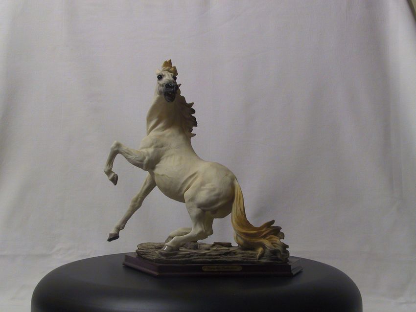
Fig. 11. When detecting a 3D object viewpoint change is more challenging due to self-occlusions and non-trivial lighting
effects. The images are taken from a database presented in [26] and cover a total range of 70 ◦ of camera rotation. They are
cropped around the object, while we used the original images in the experiments. (a) Horse dataset. (b) Vase dataset. (c) Desk
dataset. (d) Dog dataset.
invariance we require through the choice of the training samples. Ferns also let us incrementally
update the classifiers as more training samples become available as demonstrated by the SLAM
application of Section V-D. This flexibility is key to the ability to carry out offline computations
and significantly simplify and speed-up the run-time operation.
B. Ferns vs SIFT to detect 3D objects
So far we have considered that the keypoints lie on a planar object and evaluated the robustness
of Ferns with respect to perspective effects. This simplifies training as a single view is sufficient
and the known 2D geometry can be used to compute ground truth correspondences. However
most objects have truly three dimensional appearance, which implies that self occlusions and
complex illuminations effects have to be taken into account to correctly evaluate the performance
of any keypoint matching algorithm.
Recently, an extensive comparison of different keypoint detection and matching algorithms on
a large database of 3D objects has been published [26]. It was performed on images taken by a
stereo camera pair of objects rotating on a turntable. Figure 11 shows such images spanning a
November 7, 2008 DRAFT19 70 ◦ camera rotation range. We used this image database to evaluate the performance of Ferns for a variety of 3D objects. We compare our results against the SIFT detector/descriptor pair which has been found to perform very well on this database. The keypoints and the descriptors are computed using the same software as before [21]. As in [26], we obtained the ground truth by using purely geometric methods, which is possible because the cameras and the turn table are calibrated. The initial correspondences are obtained by using the trifocal geometry between the top/bottom cameras in the center view and every other camera as illustrated by Figure 12. We then reconstruct the 3D points for each such correspondence in the bottom/center camera coordinate frame and use these to form the initial tracks that span the −35 ◦ /+35 ◦ rotation range around a central view. Since the database images are separated by 5 ◦ , the tracks span 15 images each for the top and bottom cameras. We eliminate very short tracks and remaining tracks are extended by projecting the 3D point to each image and searching for a keypoint in the vicinity of the projection. Finally to increase robustness against spurious tracks formed by outliers, we eliminate tracks covering less then 30% of the views and the remaining tracks form the ground truth for the evaluation, which is almost free of outliers. Sample ground truth data is depicted by Figure 13, which shows the complex variations in patch appearance induced by the 3D structure of the objects. The training is done using views separated by 10 ◦, skipping every other frame in the ground truth data. We then use the views we skipped for testing purposes.. This geometry based sampling is shown in Figure 13. Sampling based on geometry creates uneven number of training and test samples for different keypoints as there are gaps in the tracks. The sampling could have been done differently to balance the number of test and training samples for each keypoint. However our approach to sampling closely mimics what happens in practice when training data comes from sparse views and the classifier must account for unequal numbers of training samples. We train the Ferns in virtually the same way we do in the planar case. Each track is assigned a class number and the training images are deformed by applying random affine deformations. We then use all of them to estimate the probability distributions, as discussed in Section III. 1000 random affine deformations per training image are used to train 50 Ferns of size 11. Ferns classify the test patches by selecting the track with the maximum probability. For SIFT, each test example is classified by selecting the track number of the keypoint in the training set with the nearest SIFT descriptor. November 7, 2008 DRAFT
20

Fig. 12.    Generating ground truth data for 3D object detection. Each test object contains two sequences of images taken
by the Top and Bottom cameras while the object rotates on the turntable. The camera geometry has been calibrated using a
checkerboard calibration pattern. We use 15 consecutive camera views for evaluation purposes, because it is easy to obtain high
quality calibration for this range of rotation.

   In our tests, we learn the appearance and the geometry of a 3D object from several views
and then detect it in new ones by matching keypoints. Hence the learned geometry can be used
to eliminate outliers while estimating the camera pose using the P3P algorithm [16] together
with a robust matching strategy such as RANSAC [14]. Unlike [26], we therefore do not use
the ratio test on descriptor distances or a similar heuristics to reject matches, as this might reject
correct correspondences. The additional computational burden can easily be overcome by using
the classification score for RANSAC sampling as presented by [9].
   We compare the recognition rates of both methods on objects with different kinds of texture.
Figure 14 shows the recognition rate on each test image together with the average over all
frames. The Ferns perform as well as nearest neighbor matching with SIFT for a whole range
of objects with very different textures.
   Note that, when using Ferns, there is almost no run-time speed penalty for using multiple
frames, since as more training frames are added we can increase the size of our Ferns. As
discussed in Section IV this requires more memory but does not slow down the algorithm in any

November 7, 2008                                                                                                       DRAFT
21

Fig. 13.   Samples from the ground truth for the Horse dataset. The image on the left shows the center view. The six keypoint
tracks on the right show the content variation for each patch as the camera center rotates around the turntable center. Each
track contains two lines that correspond to the Top and Bottom cameras, respectively. Black areas denote frames for which the
keypoint detector did not respond. The views produced by a rotation that is a multiple of 10 ◦ are used for training and are
denoted by red labels. The others are used for testing.

meaningful way. By contrast, using more frames for nearest neighbor SIFT matching linearly
slows down the matching, although a clever and approximate implementation might mitigate the
problem.
   In theory it should be possible to improve the performance of SIFT-based approach by
replacing nearest neighbor matching with a more sophisticated technique such as K-Nearest
Neighbors with voting. However, this would further slow down the algorithm. Our purpose is to
show that the Fern based classifier can naturally integrate data from multiple images without the
need for a more complex training phase or any handicap in the run-time performance, reaching
the performance of standard SIFT matching.

C. Panorama and 3–D Scene Annotation

   With the recent proliferation of mobile devices with significant processing power, there has
been a surge of interest in building real-world applications that can automatically annotate the
photos and provide useful information about places of interest. These applications test keypoint

November 7, 2008                                                                                                      DRAFT
22

                                                     Recognition Rate for Horse Dataset                                                                           Recognition Rate for Desk Dataset
                       1                                                                                                            1
                                                                                                                                                                                                           Average NN−SIFT
                                                                                                                                                                                                           Average Ferns
                      0.9                                                                                                          0.9

                      0.8                                                                                                          0.8

                      0.7                                                                                                          0.7

                      0.6                                                                                                          0.6
   Recognition Rate

                                                                                                                Recognition Rate
                      0.5                                                                                                          0.5

                      0.4                                                                                                          0.4

                      0.3                                                                                                          0.3

                      0.2                                                                                                          0.2

                      0.1                                                                                                          0.1
                                                                                              Average NN−SIFT
                                                                                              Average Ferns
                       0                                                                                                            0
                            1   2      3    4  5    6     7   8            1    2   3   4     5   6   7   8                              1   2      3    4  5    6     7   8            1    2   3   4     5   6   7   8

                                                     Recognition Rate for Vase Dataset                                                                            Recognition Rate for Dog Dataset
                       1                                                                                                            1
                                                                                              Average NN−SIFT                                                                                              Average NN−SIFT
                                                                                              Average Ferns                                                                                                Average Ferns
                      0.9                                                                                                          0.9

                      0.8                                                                                                          0.8

                      0.7                                                                                                          0.7

                      0.6                                                                                                          0.6
   Recognition Rate

                                                                                                                Recognition Rate

                      0.5                                                                                                          0.5

                      0.4                                                                                                          0.4

                      0.3                                                                                                          0.3

                      0.2                                                                                                          0.2

                      0.1                                                                                                          0.1

                       0                                                                                                            0
                            1   2      3    4  5    6     7   8            1    2   3   4     5   6   7   8                              1   2      3    4  5    6     7   8            1    2   3   4     5   6   7   8

Fig. 14.                    Recognition rates for 3D objects. Each pair of bars correspond to a test frame. The red bar on the left represents the
rate for Ferns and the light green bar on the right the rate for Nearest Neighbor SIFT matching. The weighted averages over
all frames also appear as dashed line for Ferns and solid line for NN-SIFT. The weights we use are the number of keypoints
per frame.

matching algorithms to their limits because they must operate under constantly changing lighting
conditions and potentially changing scene texture, both of which reduce the number of reliable
keypoints. We have tested Ferns on two such applications, annotation of panorama scenes and
parts of a historical building with 3–D structure. Both applications run smoothly at frame rate
using a standard laptop and an of the shelf web camera. By applying standard optimizations for
embedded hardware, we have ported this implementation onto a mobile device that runs at a few
frames per second. More recently, Ferns have been successfully integrated into commercially

November 7, 2008                                                                                                                                                                                                       DRAFT
23
(a)
(b)
Fig. 15. Automated image annotation (a) We match an input image against a panorama. Despite occlusions, changes in weather
conditions and lighting, the Ferns return enough matches for reliable annotation of major landmarks in the city. (b) We match
an image to an annotated 3–D model, overlaid on the two leftmost images. This lets us display annotations at the right place.
available mobile phones to run at frame rates by taking into account specific limitations of the
hardware and integrating detection with frame-to-frame tracking [34].
For the panorama application, we trained Ferns using an annotated panorama image stitched
from multiple images. At run-time given an input image and after having established correspon-
dences between the panorama and the test image, we compute a 2–D homography and use it to
eliminate outliers and to transfer the annotation from the training image to the input image as
shown in Figure 15. We successfully run a number of tests under different weather conditions
and different times of day.
Annotating a 3–D object requires training using multiple images from different viewpoints,
which is easy to do in our framework as discussed in the previous subsection. We also built a
3–D model for the object using standard structure from motion algorithms to register the training
images followed by dense reconstruction [33], [32]. The resulting fine mesh is too detailed to
be used so it is approximated by a coarse one containing much less detail. Despite its rough
structure, this 3–D model allows annotation of important parts of the object and the correct
November 7, 2008 DRAFT24 Fig. 16. Ferns applied to SLAM. (a) Initialization: The pattern at the top is detected in the image yielding initial landmarks and pose. (b) A later image from the sequence, which shows both strong camera shaking and motion blur. When the image is that bad no correspondences can be established and the tracking is lost. Nevertheless, the system automatically recovers when the image quality improves thanks to the Ferns. reprojection of this information onto images taken from arbitrary viewpoints as depicted by Figure 15. D. SLAM using Ferns In this section we demonstrate that Ferns can increase the robustness of a Visual SLAM system. Their role is twofold. We first use them to bootstrap the system by localizing the camera with respect to a known planar pattern in the scene. Second, we incrementally train a second set of Ferns to recognize new landmarks reconstructed by the system. They make the system robust against severe disturbances such as complete occlusion or strong shaking of the camera, as evidenced by the smoothness of the recovered camera trajectory in Fig. 17 (a). November 7, 2008 DRAFT
25

   For simplicity, we use a FastSLAM [24], [25] approach with a single particle to model the
distribution over the camera trajectory. This is therefore a simplified version of FastSLAM, but
the Ferns are sufficiently powerful to make it robust.
   As discussed above, we use two different sets of Ferns. We will refer to the first set as
“Offline Ferns”, that we trained offline to recognize keypoints on the planar pattern. As shown
on Figure 16 (a), we make sure it is visible in the first frame of the sequence to bootstrap
the system and replace the four fiducial markers used by many other systems. This increases
the flexibility of our system since we can use any pattern we want provided that it is textured
enough. The second set of Ferns, the “Online Ferns”, are incrementally trained to recognize the
3D landmarks the SLAM system discovers and reconstructs.
   The incremental training takes place over several frames, typically between 20 and 50, where
the corresponding landmark was matched. For each, we add a small number of random views
of the observed patch to the Ferns. In the case where a landmark is observed for the first time,
this number is substantially higher, around 100. The comparatively small number of views in the
beginning works because motion between frames are relatively small and by the time the viewing
angle has changed significantly the training will be complete. Of course, not all of the patches
need to be re-trained, but only the new ones. This is achieved by undoing the normalization step,
adding the new observations and then re-normalizing the posteriors. This incremental training is
computationally costly and future research will aim at reducing the cost of training [7].
   Our complete algorithm goes through the following steps:
   1) Initialize the camera pose and some landmarks by detecting a known pattern using the
       Offline Ferns.
   2) Detect keypoints and match them using the Offline and Online Ferns against the known
       landmarks.
   3) Estimate the camera pose from these correspondences using a P3P algorithm and RANSAC [14].
       The estimated pose is refined via a non-linear optimization.
   4) Refine the location estimates of the inlier landmarks using an Extended Kalman filter.
   5) Create new landmarks. Choose a number of detected keypoints that do not belong to any
       landmark in the map and initialize the new landmarks with a large uncertainty along the
       line of sight and a much smaller uncertainty in the camera’s lateral directions.
   6) Retrain Ferns with good matches from 2) and the new landmarks.

November 7, 2008                                                                            DRAFT
26
7) Loop to step 2.
With this system we demonstrate that both smooth tracking and recovery from complete failure
can be naturally integrated by employing Ferns for the matching task.
The reconstructed trajectory in Fig. 17 shows only tiny jags in the order of a few millimeters
and appears as smooth as a trajectory that was estimated in a filtered approach to SLAM, such as
MonoSLAM [11], [10]. This is especially noteworthy as the camera’s state is re-estimated from
scratch in every frame and there is no such thing as a motion model.2 At the same time, this is
a strong indication for an overall correct operation, since an incorrect map induces an unstable
state estimation and vice versa. In total the system mapped 724 landmarks and ran stable over
all 2026 frames of the sequence.
Recently, [35] presented a system that is also capable of recovering from complete failure.
They achieved robustness with a hybrid combination between template matching and a modified
version of Randomized Trees. However, their map typically contains one order of magnitude
fewer landmarks and there has been no indication that the modified Trees will still be capable
of handling a larger number of interest-points.
We also validated our system quantitatively. First, we checked the relative accuracy for
reconstructed pairs of 3D points and we found an error between 3.5 to 8.8% on their Euclidean
distances. Second, the absolute accuracy was assessed by choosing two world planes parallel to
the ground plane on top of two boxes in the scene on which some points were reconstructed.
Their z-coordinates deviated on average 7–10 mm. Given that the camera is at roughly 0.6 to
1.4 m from the points under consideration, this represents very good accuracy.
VI. C ONCLUSION
We have presented a powerful method for image patch recognition that performs well even
in the presence of severe perspective distortion. The “semi-naive” structure of ferns yields a
scalable, simple, and fast implementation to what is one of the most critical step in many
Computer Vision tasks. Furthermore the Ferns naturally allow trade offs between computational
complexity and discriminative power. As computers become more powerful, we can add more
2
Other systems commonly use a motion model to predict the feature location in the next frame and accordingly restrict the
search area for template matching.
November 7, 2008 DRAFT27 Ferns to improve the performance. Conversely, we can adapt them to low computational power such those on hand-held systems by reducing the number of ferns. This has actually been done in recent work [34] to achieve real-time performance on a mobile phone. A key component of our approach is the Naive-Bayesian combination of classifiers that clearly outperforms the averaging of probabilities we used in earlier work [20]. To the best of our knowledge, a clear theoretical argument motivating the superiority of Naive-Bayesian (NB) techniques does not exist. There is however strong emprical evidence that they are effective in our specific case. This can be attributed to two different causes. First, unlike mixture models, the product models can represent much sharper distributions [17]. Indeed, when averaging is used to combine distributions, the resulting mixture has higher variance than the individual components. In other words, if a single Fern strongly rejects a keypoint class, it can counter the combined effect of all the other Ferns that gives a weak positive response. This increases the necessity of larger amounts of training data and the help of a prior regularization term as discussed in Section III. Second, the classification task, which just picks a single class, will not be adversely affected by the approximation errors in the joint distribution as long as the maximum probability is assigned to the correct class [15], [12]. We have shown that such a naive combination strategy is a worthwhile alternative when the specific problem is not overly sensitive to the implied independence assumptions. November 7, 2008 DRAFT
28

Fig. 17. Ferns applied to SLAM. (a) View from top on the xy-plane of the 3D space in which the trajectory and landmarks are
reconstructed. The landmarks are shown as cubes centered around the current mean value of the corresponding Kalman filter.
Note how smooth the trajectory is, given the difficulties the algorithm had to face. (b) Qualitative visual comparison: One group
of 3D points and the corresponding group of 2D points is marked. Comparing this group to the surroundings confirmes a basic
structural correctness of the reconstruction.
November 7, 2008                                                                                                         DRAFT
29

                                                      R EFERENCES

 [1] Y. Amit. 2D Object Detection and Recognition: Models, Algorithms, and Networks. The MIT Press, 2002.
 [2] Y. Amit and D. Geman. Shape Quantization and Recognition with Randomized Trees. Neural Computation, 9(7):1545–
     1588, 1997.
 [3] J. Beis and D.G. Lowe. Shape Indexing using Approximate Nearest-Neighbour Search in High-Dimensional Spaces. In
     Conference on Computer Vision and Pattern Recognition, pages 1000–1006, Puerto Rico, 1997.
 [4] C.M. Bishop. Pattern Recognition and Machine Learning. Springer, 2006.
 [5] Alexander Böcker, Swetlana Derksen, Elena Schmidt, Andreas Teckentrup, and Gisbert Schneider. A Hierarchical Clustering
     Approach for Large Compound Libraries. Journal of Chemical Information and Modeling, 45:807–815, 2005.
 [6] A. Bosch, A. Zisserman, and X. Munoz. Image classification using random forests and ferns. In International Conference
     on Computer Vision, 2007.
 [7] M. Calonder, V. Lepetit, and P. Fua. Keypoint signatures for fast learning and recognition. In European Conference on
     Computer Vision, Marseille, France, October 2008.
 [8] C. Chow and C. Liu. Approximating discrete probability distributions with dependence trees. Information Theory, IEEE
     Transactions on, 14(3):462–467, 1968.
 [9] O. Chum and J. Matas. Matching with PROSAC - Progressive Sample Consensus. In Conference on Computer Vision
     and Pattern Recognition, pages 220–226, San Diego, CA, June 2005.
[10] A. J. Davison, I. Reid, N. Molton, and O. Stasse. Monoslam: Real-time single camera slam. IEEE Transactions on Pattern
     Analysis and Machine Intelligence, 29(6):1052–1067, June 2007.
[11] Andrew J. Davison. Real-Time Simultaneous Localisation and Mapping with a Single Camera. ICCV, 02:1403, 2003.
[12] Pedro Domingos and Gregory Provan. On the optimality of the simple bayesian classifier under zero-one loss. Machine
     Learning, 29:103—130, 1997.
[13] L. Fei-Fei, R. Fergus, and P. Perona. One-shot learning of object categories. IEEE Transactions on Pattern Analysis and
     Machine Intelligence, 28(4):594–611, 2006.
[14] M.A Fischler and R.C Bolles. Random Sample Consensus: A Paradigm for Model Fitting with Applications to Image
     Analysis and Automated Cartography. Communications ACM, 24(6):381–395, 1981.
[15] Jerome H Friedman and Usama Fayyad. On bias, variance, 0/1-loss, and the curse-of-dimensionality. Data Mining and
     Knowledge Discovery, 1:55—77, 1997.
[16] X.-S. Gao, X.-R. Hou, J. Tang, and H.-F. Cheng. Complete solution classification for the perspective-three-point problem.
     IEEE Trans. Pattern Anal. Mach. Intell., 25(8):930–943, 2003.
[17] G.E. Hinton. Training products of experts by minimizing contrastive divergence. Neural Computation, 14:1771–1800,
     2002.
[18] Derek Hoiem, Rahul Sukthankar, Henry Schneiderman, and Larry Huston. Object-based image retrieval using the statistical
     structure of images. Conference on Computer Vision and Pattern Recognition, 02:490–497, 2004.
[19] J. Kittler, M. Hatef, R.P.W. Duin, and J. Matas. On Combining Classifiers. IEEE Transactions on Pattern Analysis and
     Machine Intelligence, 20(3):226–239, 1998.
[20] V. Lepetit and P. Fua. Keypoint recognition using randomized trees. IEEE Transactions on Pattern Analysis and Machine
     Intelligence, 28(9):1465–1479, September 2006.
[21] D. Lowe. Demo software: Sift keypoint detector, 2008. http://www.cs.ubc.ca/˜lowe/keypoints/.

November 7, 2008                                                                                                      DRAFT
You can also read