Melting and fragmentation laws from the evolution of two large Southern Ocean icebergs estimated from satellite data - The Cryosphere
←
→
Page content transcription
If your browser does not render page correctly, please read the page content below
The Cryosphere, 12, 2267–2285, 2018
https://doi.org/10.5194/tc-12-2267-2018
© Author(s) 2018. This work is distributed under
the Creative Commons Attribution 4.0 License.

Melting and fragmentation laws from the evolution of two large
Southern Ocean icebergs estimated from satellite data
Nicolas Bouhier1 , Jean Tournadre1 , Frédérique Rémy2 , and Rozenn Gourves-Cousin1
1 Laboratoire d’Océanographie Physique et Spatiale, UMR 6523, IFREMER, CNRS, IRD, Université Bretagne-Loire,
Plouzané, France
2 Laboratoire d’Etudes en Géophysique et Océanographie Spatiales, UMR 5566, CNES – CNRS, Toulouse, France

Correspondence: Jean Tournadre (jean.tournadre@ifremer.fr)

Received: 15 September 2017 – Discussion started: 14 November 2017
Revised: 21 June 2018 – Accepted: 22 June 2018 – Published: 12 July 2018

Abstract. The evolution of the thickness and area of two           the Southern Ocean by large icebergs (i.e. > 18 km in
large Southern Ocean icebergs that have drifted in open wa-        length). However, their basal melting, that is of the order
ter for more than a year is estimated through the combined         of 320 km3 yr−1 , accounts for less than 20 % of their mass
analysis of altimeter data and visible satellite images. The ob-   loss, and the majority of ice loss (1500 km3 r −1 ∼ 80 %) is
served thickness evolution is compared with iceberg melting        achieved through breaking into smaller icebergs (Tournadre
predictions from two commonly used melting formulations,           et al., 2016). Large icebergs actually act as a reservoir to
allowing us to test their validity for large icebergs. The first   transport ice away from the Antarctic coastline into the ocean
formulation, based on a fluid dynamics approach, tends to          interior, while fragmentation can be viewed as a diffusive
underestimate basal melt rates, while the second formulation,      process. It generates plumes of small icebergs that melt far
which considers the thermodynamic budget, appears more             more efficiently than larger ones that have a geographical dis-
consistent with observations. Fragmentation is more impor-         tribution that constrains the input into the ocean.
tant than melting for the decay of large icebergs. Despite its        Global ocean models that include iceberg components
importance, fragmentation remains poorly documented. The           (Gladstone et al., 2001; Jongma et al., 2009; Martin and Ad-
correlation between the observed volume loss of our two ice-       croft, 2010; Marsh et al., 2015; Merino et al., 2016) show that
bergs and environmental parameters highlights factors most         basal ice-shelf and iceberg melting have different effects on
likely to promote fragmentation. Using this information, a         the ocean circulation. Numerical model runs with and with-
bulk model of fragmentation is established that depends on         out icebergs show that the inclusion of icebergs in a fully
ocean temperature and iceberg velocity. The model is ef-           coupled general circulation model (GCM) results in signif-
fective at reproducing observed volume variations. The size        icant changes in the modelled ocean circulation and sea-ice
distribution of the calved pieces is estimated using both al-      conditions around Antarctica (Jongma et al., 2009; Martin
timeter data and visible images and is found to be consis-         and Adcroft, 2010; Merino et al., 2016). The transport of ice
tent with previous results and typical of brittle fragmentation    away from the coast by icebergs and the associated freshwa-
processes. These results are valuable in accounting for the        ter flux cause these changes (Jongma et al., 2009). Although
freshwater flux constrained by large icebergs in models.           the results of these modelling studies are not always in agree-
                                                                   ment in terms of ocean circulation or sea ice extent they all
                                                                   highlight the important role that icebergs play in the climate
                                                                   system, and they also show that models that do not include
1   Introduction                                                   an iceberg component are effectively introducing systematic
                                                                   biases (Martin and Adcroft, 2010).
According to recent studies (Silva et al., 2006; Tournadre            However, despite these modelling efforts, the current gen-
et al., 2015, 2016), most of the total volume of ice ( ∼ 60 %)     eration of iceberg models are not yet able to represent the
calved from the Antarctic continent is transported into

Published by Copernicus Publications on behalf of the European Geosciences Union.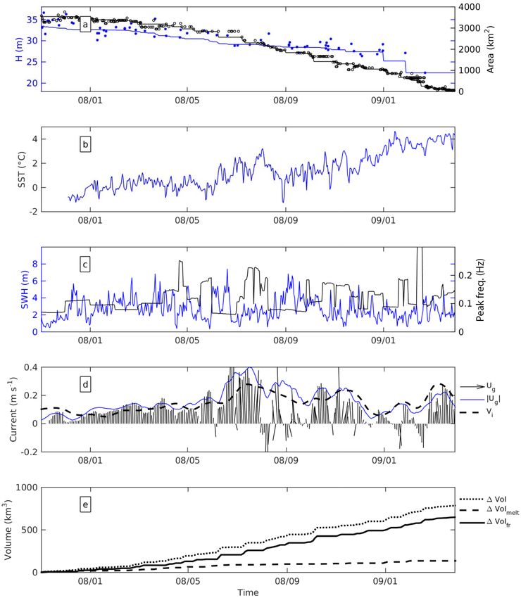
2268                                                                 N. Bouhier et al.: Iceberg melting and fragmentation

full range of iceberg sizes observed in nature from growlers      tribution of icebergs calved from large Southern Ocean ice-
(≤ 10 m) to “giant” tabular icebergs (≥ 10 km).                   bergs.
   The iceberg size distribution has also strong impact on           Recent progress in satellite altimeter data analysis allows
both circulation and sea ice as shown by Stern et al. (2016).     us to estimate the small (< 3 km in length) iceberg distribu-
Furthermore, all current iceberg models fail in accounting for    tion and volume as well as the freeboard elevation profile and
the size transfer of ice induced by fragmentation, as in these    volume of large icebergs (Tournadre et al., 2016). The loca-
models small icebergs cannot stem from the breaking of big-       tion, area, and volume of small icebergs from 1992 to 2018
ger ones.                                                         is contained in a database distributed by CERSAT, as well as
   The two main decay processes of icebergs, melting and          monthly fields of probability of presence, mean area and vol-
fragmentation, are still quite poorly documented and not          ume of ice (Tournadre et al., 2016). It is now possible to es-
fully represented in numerical models. Although iceberg           timate the thickness variations and thus the melting of large
melting has been widely studied (Huppert and Josberger,           icebergs. A crude estimate of the large iceberg area is also
1980; Neshyba, 1980; Hamley and Budd, 1986; Jansen et al.,        available from the National Ice Center but it is not precise
2007; Jacka and Giles, 2007; Helly et al., 2011), very few        enough to allow analysis of the area lost by fragmentation.
validations of melting laws have been published (Jansen           A more precise area analysis can be conducted by analysing
et al., 2007), especially for large icebergs. Large uncertain-    satellite images such as those for the Moderate Resolution
ties still remain for the melting laws to be used in numerical    Imaging Spectroradiometer (MODIS) onboard the Aqua and
models.                                                           Terra satellites (Scambos et al., 2005).
   The calving of icebergs from glaciers and ice shelves has         Two large icebergs, B17a and C19a, which have drifted
been quite well studied (e.g. Holdsworth and Glynn, 1978;         for more than one year in open water (see Fig. 1) away from
Fricker et al., 2002; Benn et al., 2007; MacAyeal et al., 2006;   other large icebergs and which have been very well sampled
Amundson and Truffer, 2010) and empirical calving laws            by altimeters and MODIS, have been selected to study the
have been proposed (Amundson and Truffer, 2010; Bassis,           melting and fragmentation of large Southern Ocean tabular
2011). However, very few studies have been dedicated to           icebergs. Their freeboard evolution, and thus thickness, is
the breaking of icebergs. Analysing the decay of Green-           estimated from satellite altimeter data, while their area and
land icebergs, Savage (2001) proposed three distinct frag-        shape have been estimated from the analysis of MODIS im-
mentation mechanisms. Firstly, flexural breakups by swell         ages. The icebergs area and thickness evolution is then used
induced vibrations, in the frequency range of the iceberg bob-    to test the validity of the melting models used in iceberg
bing on water, that could cause fatigue and fracture at weak      numerical modelling and to analyse the fragmentation pro-
spots (Goodman et al., 1980; Schwerdtfeger, 1980; Wad-            cess. The two icebergs were also chosen because they have
hams et al., 1983). Secondly, two mechanisms resulting from       very different characteristics. While C19a was one of the
wave erosion at the waterline, calving of ice overhangs and       largest iceberg on record (> 1000 km2 ) and drifted for more
buoyant footloose mechanism (Wagner et al., 2014). Scam-          than 2 years in the South Pacific, B17a was relatively small
bos et al. (2008), using satellite images, ICESat altimeter and   (200 km2 ) and drifted in the Weddell Sea. The large plumes
field measurements analysed the evolution of two Antarc-          of small icebergs generated by the decay of both large ice-
tic icebergs and identified three styles of calving during the    bergs can be detected by altimeters and MODIS images. The
drift: “rift calving”, which corresponds to the calving of        ALTIBERG database and selected MODIS images can be
large daughter icebergs by fracturing along preexisting flaws,    used to analyse the size distribution of fragments.
“edge wasting”, the calving of numerous small narrow ice-            The present paper is organized as follows. Section 2 de-
bergs and “rapid disintegration”, which is characterized by       scribes the data used in the study, including the environmen-
the rapid calving of numerous icebergs.                           tal parameters (such as ocean temperature, current speed,
   The pieces calved from icebergs drift away from their par-     etc.) necessary to estimate melting and fragmentation. Sec-
ent under the action of wind and ocean currents as a function     tion 3 presents the evolution of the two selected icebergs. In
of size, shape, and draft (Savage, 2001). This dispersion can     Sect. 4, the two melting laws widely used in the literature,
create large plumes of icebergs that can represent a signifi-     forced convection and thermal turbulence exchange, are con-
cant contribution to the freshwater flux over vast oceanic re-    fronted with the observed melting of B17a and C19a. The fi-
gions where no large icebergs are observed (Tournadre et al.,     nal section analyses the fragmentation process and proposes
2016). The size distribution of the calved pieces is needed to    a fragmentation law. It also investigates the size distribution
analyse and understand the transfer of ice between the differ-    of pieces calved from large icebergs.
ent iceberg scales and thus to estimate the freshwater flux.
It is also important for modelling purposes. Savage et al.
(2000), using aerial images and in situ measurements, es-
timated the size distribution of small bergy bits (< 20 m in
length) calved from deteriorating Greenland icebergs. How-
ever, until now, no study has been published on the size dis-

The Cryosphere, 12, 2267–2285, 2018                                                   www.the-cryosphere.net/12/2267/2018/
N. Bouhier et al.: Iceberg melting and fragmentation                                                                                                            2269

                       55° W   50° W   45° W   40° W
               60° W
                                                       35° W

                                                                                                                150° W   135° W
 52° S                                                                                                 165° W                                                   Jan 09
                                                               Feb 15                                                             120° W
                   a                                           Oct 14
                                                                                              180° W
    54°    S                                                                                                                               105° W               Jul 08

                                                               Jul 14
     56°   S                                                                     165° E                                                                         Dec 07
                                                               Apr 14                                                                                 90° W
      58° S                                                                               b
                                                                                                                                                                Jun 07
                                                               May 15                                                                                   55° S
                                                                        150° E
                                                               Feb 15
          60° S                                                                                                                                     60° S       Nov 06

                                                               Oct 14
                                                                                                                                             65° S
           62° S                                                                                                                                                May 06
                                                               Jul 14

           64° S                                               Apr 14

               66° S

Figure 1. Trajectories of B17a (a) and C19a (b) icebergs. The black circle locates the B17a grounding site. The colour scale represents the
time along the trajectory.

2     Data                                                                                volume of all the NIC and BYU large icebergs covering the
                                                                                          2002–2012 period. For example, B17a was sampled by 152
2.1        Iceberg data                                                                   altimeter passes during its drift and C19a by 258 passes (see
                                                                                          Fig. 2).
The National Ice Center (NIC) Southern Hemisphere Iceberg
Database contains the position and size (length and width),                               2.2    Visible images
estimated by analysis of visible or SAR images of icebergs
larger than 10 nautical miles (19 km) along at least one axis;                            The weekly estimates of iceberg lengths and widths pro-
it is updated weekly. Every iceberg is tracked, and when im-                              vided by NIC are manually estimated from satellite images
agery is available, information is updated and posted. The                                and they are not accurate enough to precisely compute the
Brigham Young University (BYU) Center for Remote Sens-                                    iceberg area and its evolution. A careful re-analysis of the
ing maintains an Antarctic Iceberg Tracking Database for                                  MODIS imagery from the Aqua and Terra satellites was thus
icebergs larger than 6 km in length (Stuart and Long, 2011).                              conducted to precisely estimate the C19a and B17a area until
Using six different satellite scatterometer instruments, they                             their final detectable collapse. The images have been system-
produced an iceberg tracking database that includes icebergs                              atically collocated with the two icebergs using the NIC/BYU
identified in enhanced resolution scatterometer backscatter.                              track data. It should be noted that in some areas of high ice-
The initial position for each iceberg is located based on a po-                           berg concentration, especially when B17a reaches the “ice-
sition reported by the NIC or by the sighting of a moving                                 berg alley”, NIC and BYU regularly mistakenly followed an-
iceberg in a time series of scatterometer images.                                         other iceberg, or lost its track when it became quite small.
    In 2007, Tournadre (2007) demonstrated that any target                                Here, more than 1500 images were collocated and selected.
emerging from the sea surface (such as an iceberg) can pro-                               The level 1B calibrated radiances from the two higher res-
duce a detectable signature in high-resolution altimeter wave                             olution (250 m) channels (visible channels 1 and 2 at 645
forms. Their method enables us to detect icebergs in open                                 and 860 nm frequencies, respectively) were used to estimate
ocean only, and to estimate their area. Due to constraints on                             the iceberg’s characteristics. For each image with good cloud
the method, only icebergs between 0.1 and ∼ 9 km2 can be                                  clover and light conditions, a supervised shape analysis was
detected. Nine satellite altimetry missions have been pro-                                performed. Firstly, a threshold depending on the image light
cessed to produce a 1992–2018 database of small iceberg                                   conditions is estimated and used to compute a binary im-
locations, area, volume, and mean backscatter (Tournadre                                  age. The connected components of the binary image are then
et al., 2016). The monthly mean probability of presence, area                             determined using standard Matlab© image processing tools
and volume of ice over a regular polar (100 × 100 km2 ) or                                and finally the iceberg’s properties, centroid position, major
geographical (1◦ × 2◦ ) grid are also available and are dis-                              and minor axis lengths, and area are estimated. On a number
tributed on the CERSAT website.                                                           of occasions, the iceberg’s surface was obscured by clouds,
    Altimetry can also be used to measure the freeboard ele-                              but visual estimation was possible because the image con-
vation profile of large icebergs (McIntyre and Cudlip, 1987;                              trast was sufficient to discern edges through clouds. For these
Tournadre et al., 2015). Combining iceberg tracks from NIC                                instances, the iceberg’s edge and shape were manually esti-
and the archives of three Ku band altimeters, Jason-1, Jason-                             mated. The final analysis is based on 286 valid images for
2, and Envisat, Tournadre et al. (2015) created a database                                B17a, and 503 for C19a. The locations of the MODIS images
of daily position, freeboard profile, length, width, area, and                            for B17a and C19a are given in Fig. 2 while four examples

www.the-cryosphere.net/12/2267/2018/                                                                               The Cryosphere, 12, 2267–2285, 2018
2270 N. Bouhier et al.: Iceberg melting and fragmentation
°
° 50 W 45° W 40° W
60° W 55 W °
35 W
° 150° W
140° W °
52° S 170° 160 W
W
130 W °
a ° 120 W °
180 W 110 W
54° S ° °
170 E 100 W
56° S °
160 E b °
90 W
°
58 S
°
150 E 55°
°
60 S
°
60 S 65° S
62° S
64° S
°
66 S
Figure 2. Sampling of B17a (a) and C19a (b) icebergs by MODIS (beige stars) and altimeters (blue circles).
of iceberg area estimates are given in Fig. 3. The comparison 3 Melting and fragmentation of B17a and C19a
of area for consecutive images shows that the area precision
is around 2–3 %. 3.1 B17a
2.3 Environmental data Iceberg B17a originates from the breaking of giant tab-
ular B17 near Cape Hudson in 2002. It then drifted for
Several environmental parameters along the icebergs trajec- 10 years along the continental slope within the “coastal cur-
tories are also used in this study. Due to the lack of a bet- rent”, until it reached the Weddell Sea in summer 2012
ter alternative, the sea surface temperature (SST) is used as (see Fig. 1a). It travelled within sea ice at a speed ranging
a proxy for the water temperature. The difference between from 2 to 12 cm s−1 , coherent with previous observational
the SST and the temperature at the base of the iceberg will studies (Schodlok et al., 2006). It crossed the Weddell Sea
introduce an error in the melt rate computation, as shown while drifting within sea ice and reached the open water
by Merino et al. (2016). Using results from an Ocean Gen- in April 2014. It was then caught in the western branch of
eral Circulation Model, they also compared the mean SST the Weddell Gyre and drifted north in the Scotia Sea until
and the average temperature over the first 150 m from the it grounded, in October 2014, near South Georgia, a com-
surface showing that the mean difference is less than 0.5 ◦ C mon grounding spot for icebergs. It remained there for almost
for most of the Southern Ocean. The level-4 satellite analy- 6 months until it finally left its trap in March 2015 and drifted
sis product ODYSSEA, distributed by the Group for High- back northward until its final demise in early June 2015.
Resolution Sea Surface Temperature (GHRSST) has been B17a was a “medium size” big iceberg, with primary dimen-
used. It is generated by merging infrared and microwave sen- sions of 35 × 14 km2 and an estimated freeboard of 52 m, re-
sors and using optimal interpolation to produce daily cloud- sulting in an original volume of 113 km3 and a corresponding
free SST fields at 10 km resolution over the globe. The sea mass of ∼ 103 Gt. Before 2014, B17a freeboard and area re-
ice concentration data are from the CERSAT level-3 daily mained almost constant while it drifted within sea ice. After
concentration product, available on a 12.5 km polar stereo- March 2014, B17a started to drift in open water and to melt
graphic grid from the SSM/I radiometer observations. The and break. During its drift in open water, from March 2014
wave height and wave peak frequencies come from the global to June 2015, B17a was sampled by 200 MODIS images and
Wave Watch3 hindcast products from the IOWAGA project 41 altimeter passes. Figure 4a presents the satellite freeboard
(http://wwz.ifremer.fr/iowaga/, last access: September 2017). and area measurements as well as the daily interpolated val-
The AVISO Maps of Absolute Dynamic Topography & abso- ues. The standard deviation of freeboard estimate computed
lute geostrophic velocities (MADT) provides a daily multi- from the freeboard elevation profiles is ±3 m. The standard
mission absolute geostrophic current on a 0.25◦ regular grid deviation of the iceberg area has been estimated by analysing
that is used to estimate the current velocities at the iceberg the area difference between images taken the same day. It is
locations. of the order of 3–4 %. During this drift in the Weddell Sea,
it experienced different basal melting regimes: firstly, when
it left the peninsula slope current, with negative SSTs and
low drift speeds (see Fig. 4b and d), it was subject to an av-
erage melt rate of 5.7 m month−1 , then drifted more rapidly
within the Scotia Sea and experienced a mean thickness de-
The Cryosphere, 12, 2267–2285, 2018 www.the-cryosphere.net/12/2267/2018/N. Bouhier et al.: Iceberg melting and fragmentation 2271
Figure 3. Example of B17a (a, b) and C19a (c, d) area estimate using MODIS images. The blue lines represent the iceberg perimeter and
the red and green crosses represent the NIC and MODIS iceberg’s positions, respectively.
crease of 15 m month−1 , and finally it melted at a rate close For large icebergs, the sidewall erosion and melting, which
to 20 m month−1 as it accelerated its drift before its ground- is of the order of some metres per day, can be considered
ing. As for fragmentation, the area loss was limited (40 km2 negligible compared to breaking. As B17a started to drift in
in 250 days, i.e. less than 10 %) but then accelerated as B17a open water, its mass varied slowly at first, mainly through
became trapped (80 km2 in 70 days). The area loss slowed melting. Between January 2014 and March 2015, basal melt-
down for the second half of the grounding, only to increase ing accounted for more than 60 % of the total volume loss,
dramatically once B17a was released and before it collapsed whereas fragmentation was responsible for 30 % of the loss.
a few days later. This could be related to an embrittlement of However, after November 2014 breaking became dominant
the iceberg structure, potentially under the influence of un- as the iceberg started to break up more rapidly.
balanced buoyancy forces while grounded (Venkatesh, 1986;
Wagner et al., 2014; Stern et al., 2015). 3.2 C19a
The cumulative total volume loss, basal melting, breaking
are presented in Fig. 4e. These terms are computed from the Our second iceberg of interest is the giant C19a which was
mean thickness and area as follows: the basal melting volume one of the fragments resulting from the splitting of C19, the
loss M at day i is the sum of the products of iceberg surface, second largest tabular iceberg on record. C19a was born off-
S (in m2 ), by the daily variation of thickness, dT shore of Cape Adare (170◦ E) in 2003 and was originally ob-
i
long and narrow, around 165 km long and 32 km wide with
an estimated freeboard of ∼ 40 m, i.e. a volume of about
X
M(i) = S(k)dT (k), (1)
k=1 1000 km3 and a mass of 900 Gt. It drifted mainly in a north-
easterly direction for almost 4 years, most of the time in sea
and the breaking loss B (in m3 ) is the sum of the products of ice, until it first entered the open ocean in summer 2005 (see
thickness, T , by the daily variation of surface, dS Fig. 1). It was temporarily re-trapped by the floes in win-
i
ter 2006 and eventually left the ice coverage permanently
in late spring 2007. It then drifted within the Antarctic Cir-
X
B(i) = dS(k)T (k). (2)
k=1 cumpolar Current and eventually close to the Polar Front and
www.the-cryosphere.net/12/2267/2018/ The Cryosphere, 12, 2267–2285, 20182272 N. Bouhier et al.: Iceberg melting and fragmentation
50 300
40
(a)
Area (km )
2
200
H (m)
30
20
100
10
0 0
14/03 14/05 14/07 14/09 14/11 15/01 15/03 15/05
4
2
(b)
SST ( C)
o
0
-2
14/03 14/05 14/07 14/09 14/11 15/01 15/03 15/05
10
(c) 0.2
Peak freq. (Hz)
SWH (m)
5
0.1
0 0
14/03 14/05 14/07 14/09 14/11 15/01 15/03 15/05
0.4
(d) Ug
Current (m s -1 )
0.2 |U g |
V
i
0
-0.2
14/03 14/05 14/07 14/09 14/11 15/01 15/03 15/05
100
Δ Vol
(e)
Volume loss (km 3 )
Δ Vol melt
Δ Vol fr
50
0
14/03 14/05 14/07 14/09 14/11 15/01 15/03 15/05
Time
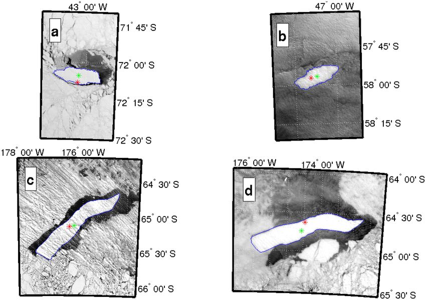
Figure 4. (a) B17a area (in km2 ) and freeboard (in m). The black and blue lines represent the interpolated daily area and freeboard and
the black circles and blue crosses the MODIS area and altimeter freeboard estimates. (b) ODYSSEA sea surface temperature (in ◦ C).
(c) Significant wave height in m (blue line) and peak frequency in Hz (green line). (d) AVISO geostrophic current (black arrows), current
velocity (blue line), and iceberg velocity (dashed black line). (e) Total volume loss (dotted line), volume loss by melting (dashed line), and
by fragmentation (solid line).
its warm waters until its final demise in April 2009 in the of the total volume decrease (see Fig. 5e). B17 thickness loss
Bellingshausen Sea. Before November 2007, C19a experi- was almost 5 times faster than that of C19, the latter experi-
enced very little change except a very mild melting (not pre- encing mean basal melt rates ranging from 1 to 3 m month−1
sented in the figure). Its volume was 880 km3 (∼ 790 Gt) in in most of its drift (and as much as 13 m month−1 in its last
December 2007 when it finally entered the open sea. During month, which was characterized by very high water temper-
its final drift, from December 2007 to March 2009, C19a was atures). As for fragmentation, its main volume loss mecha-
sampled by 317 MODIS images and 69 altimeter passes (see nism (75 %), its area loss was first mild while it progressed
Fig. 2b). The C19a area and freeboard are presented in Fig. 5 in colder waters (around 2.6 km2 day−1 ), and started to in-
as well as SST, sea state, and volume loss. While the vol- crease as soon as it entered positive temperature waters, with
ume loss was mainly due to melting before this date, break- an average loss of 9.5 km2 day−1 and with dramatic shrink-
ing dominated afterwards. Basal melting only explains 25 %
The Cryosphere, 12, 2267–2285, 2018 www.the-cryosphere.net/12/2267/2018/N. Bouhier et al.: Iceberg melting and fragmentation 2273
ages of 340 km and 370 km2 , lost in 10 days that correspond During its travel the iceberg’s surface temperature will de-
to large fragmentation events. pend on the ablation rate. When ablation is limited, i.e. in
cold waters, the ice can theoretically warm up to 0 ◦ C, while
in warmer waters the rapid disappearance of the outer lay-
4 Melting models ers tends to leave colder ice near the surface. The surface ice
temperature could thus theoretically vary from −20 to 0 ◦ C
Apart from fragmentation, the basal melting of icebergs ac- but is commonly taken at −4 ◦ C (Løset, 1993; Martin and
counts for the largest part of the total mass loss (Martin and Adcroft, 2010; Gladstone et al., 2001).
Adcroft, 2010; Tournadre et al., 2015). Although firn densi- The mean daily iceberg speed can be easily estimated
fication (see Appendix A1 for an estimate of the associated from the iceberg track. Numerical ocean circulation models
freeboard change) and surface melting can also contribute, it are not precise enough to provide realistic current speed in
is the main cause of thickness decrease. It can mainly be at- this region. The comparison of iceberg velocities and AVISO
tributed to the turbulent heat transfer arising from the differ- geostrophic currents presented in Figs. 4d and 5d shows that
ence of speed between the iceberg and the surrounding water. the iceberg velocity is sometimes significantly larger than the
Two main approaches have been used to compute the melting AVISO velocities. They are thus not reliable enough to com-
rate and to model the evolution of iceberg and the freshwa- pute the melt rate. Vw is thus treated as unknown.
ter flux (see for example Bigg et al., 1997; Gladstone et al., The basal melt is computed using Eq. (3) for Vw from 0
2001; Silva et al., 2006; Jongma et al., 2009; Merino et al., to 3 m s−1 by 0.01 steps and Ti from −20 to 2 ◦ C by 0.1 ◦ C
2016; Jansen et al., 2007). The first one is based on the forced steps. The positive temperatures are used to test the model’s
convection formulation proposed by Weeks and Campbell convergence. The uncertainties in the different parameters
(1973), while the second one uses the thermodynamic for- and measurements are too large for a direct comparison of the
mulation of Hellmer and Olbers (1989) and the turbulent ex- modelled and measured daily melt rate. However, it is possi-
change velocity at the ice-ocean boundary. The first model ble to test the model validity by comparing the bulk melting
has been exclusively used to compute iceberg basal melt rate rate, i.e. the modelled and measured cumulative loss of thick-
while the second model has been primarily developed and n M (t ).
ness, 6i=1 b i
used to estimate ice shelf melting. The B17a and C19a data As current velocities and iceberg temperatures are not con-
sets allow us to confront these two formulations with melting stant during the iceberg’s drift, the modelled thickness loss is
measurements for two icebergs of different shapes and sizes fitted to the measured loss for each time step ti over a ±20-
and under different environmental conditions and to test their day period by selecting the Vw (ti ) and Ti (ti ) that minimize
validity for large icebergs. the distance between model and observations. When no SST
is available, i.e. when the iceberg is within sea ice for a short
4.1 Forced convection of Weeks and Campbell period, Tw is fixed to the sea water freezing temperature.
The model allows us to reproduce the thickness variations
The forced convection approach of Weeks and Campbell
extremely well, with correlations larger than 0.999 for both
(1973) is based on the fluid mechanics formulation of the
B17a and C19a (see Figs. 6a and 7a) and mean differences
heat-transfer coefficient for a fully turbulent flow of fluid
of thickness loss of 3.1 and 0.5 m, respectively, and maxi-
over a flat plate. The basal convective melt rate Mb is a func-
mum differences less than 8 and 1.5 m. However, the cur-
tion of both temperature and velocity differences between the
rent velocity inferred from the model, presented in Figs. 6b
iceberg and the ocean. It is expressed (in m day−1 ) as follows
and 7b, reaches very high and unrealistic values (> 2 m s−1 ).
(Gladstone et al., 2001; Bigg et al., 1997):
Compared to the altimeter geostrophic currents from AVISO,
Tw − Ti the current speed can be overestimated by more than a fac-
Mb = C|V w − V i |0.8 , (3) tor of 10.
L0.2
The second model parameter Ti (see Figs. 6c and 7c)
with V w being the current speed (at the base of the ice- varies between −20 and −0.6 ◦ C with a −10.9 ± 7.1 ◦ C
berg), V i the iceberg speed, Ti and Tw the iceberg and water mean for B17a. For C19a, it is between −9 and 1 ◦ C with a
temperature, L the iceberg’s length (longer axis) and C = −10.6 ± 5.8 ◦ C mean, although the model sometimes fails to
0.58 K−1 m0.4 s0.8 day−1 . This expression has been widely converge to realistic iceberg temperature, i.e. for Ti < 0 ◦ C. It
used in numerical models (Bigg et al., 1997; Gladstone et al., happens when the measured melting is weak and SST is pos-
2001; Martin and Adcroft, 2010; Merino et al., 2016; Wagner itive (for example from January to May 2007, Figs. 7c and
et al., 2017). As water temperature at keel depth is not avail- 5b). The model can reproduce this inhibition by decreasing
able, the sea surface temperature (SST) is used as a proxy. the water and ice temperature difference up to zero, resulting
The SST for each iceberg is presented in Figs. 4b and 5b. in an artificial increase of the iceberg temperature to positive
The first unknown quantity in Eq. (3), the iceberg’s tempera- values. For B17a, the model always converges, and the lower
ture Ti , can be at the time of calving as low as −20 ◦ C (Die- temperatures (−20 ◦ C) are observed during extremely rapid
mand, 2001). Icebergs can sometimes drift for several years. melting period or during the grounding period. This could
www.the-cryosphere.net/12/2267/2018/ The Cryosphere, 12, 2267–2285, 20182274 N. Bouhier et al.: Iceberg melting and fragmentation
Figure 5. (a) C19a area (in km2 ) and freeboard (in m). The black and blue lines represent the interpolated daily area and freeboard, and
the black circles and blue crosses the MODIS area and altimeter freeboard estimates. (b) ODYSSEA sea surface temperature (in ◦ C).
(c) Significant wave height in m (blue line) and peak frequency in Hz (green line). (d) AVISO geostrophic current (black arrows), current
velocity (blue line) and iceberg velocity (dashed black line). (e) Total volume loss (dotted line), volume loss by melting (dashed line), and
by fragmentation (solid line).
reflect the decrease of ice surface temperature during rapid tive heat flow through the ice:
ablation events or an underestimation of the melt rate.
ρw Cpw γT (Tb − Tw ) = ρi LMb − ρi Cpi 1T Mb . (4)
4.2 Thermal turbulent exchange of Hellmer and Olbers Thus,
ρw Cw γT Tb − Tw
Mb = , (5)
The second melt rate formulation is based on thermodynam- ρi LH − Cpi 1T
ics, and on heat and mass conservation equations. It assumes
heat balance at the iceberg–water interface and was origi- where Mb is the melt rate (in m s−1 ), LH = 3.34×10⁵ J kg−1
nally formulated for estimating ice shelf melting (Hellmer is the fusion latent heat, and Cpw = 4180 J kg−1 K−1 and
and Olbers, 1989; Holland and Jenkins, 1999). The turbulent Cpi = 2000 J kg−1 K−1 are the heat capacity of seawater and
heat exchange is thus consumed by melting and the conduc- ice, respectively. Tb = −0.0057 Sw +0.0939–7.64 × 10⁻⁴ Pw
The Cryosphere, 12, 2267–2285, 2018 www.the-cryosphere.net/12/2267/2018/N. Bouhier et al.: Iceberg melting and fragmentation 2275
300
a
Thickness loss (m)
Δ Th
200
Δ Th conv
Δ Th γ
100
0
14/03 14/05 14/07 14/09 14/11 15/01 15/03
Vi
10 0 b
V conv
Speed (m s -1 )
Vγ
10 -1
V geo
10 -2
14/03 14/05 14/07 14/09 14/11 15/01 15/03
0
c
T conv
Temperature ( o C)
-5
i
-10 T γI
-15
-20
14/03 14/05 14/07 14/09 14/11 15/01 15/03
Time
Figure 6. Thickness loss (in m) for B17a (a). Measured thickness loss (black line); modelled loss using forced convection (dashed blue line)
and turbulent exchange (solid blue line). (b) Iceberg velocity (dotted black line). Modelled velocity using forced convection (solid blue line)
and using turbulent exchange (dotted blue line). AVISO Geostrophic current velocity (solid black line). (c) Modelled iceberg temperature
using forced convection (dashed line) and using thermal exchange (solid line).
is the freezing temperature at the base of the iceberg, Sw (in and found γT ranging from 0.4 × 10⁻⁴ to 1.8 × 10⁻⁴ m s−1
g kg−1 ) and Pw (in 104 Pa) are the salinity (here fixed at the close to the 1 × 10⁻⁴ m s−1 proposed by Holland and Jenk-
averaged value of 35 g kg−1 ) and pressure at the bottom of ins (1999). Silva et al. (2006), who estimated the Southern
the iceberg, 1T = Ti − Tb represents the temperature gradi- Ocean freshwater flux by combining the NIC iceberg data
ent within the ice at the iceberg base (Jansen et al., 2007). base and a model of iceberg thermodynamics also based on
γT is the thermal turbulent velocity that can be expressed as this formulation, considered a unique and much larger γT of
follows (Kader and Yaglom, 1972): 6 × 10⁻⁴ m s−1 .
The basal melt is thus computed using Eq. (5) for γT from
u∗ 0.1 × 10⁻⁵ to 10 × 10−4 m s−1 by 0.1 × 10−5 steps and Ti
γT = 2/3
, (6)
2.12 log(u∗ lν −1 ) + 12.5Pr −9 from −20 to 2 ◦ C by 0.1 ◦ C steps. As for forced convection,
the model is fitted for each time step over a ±20 day period to
where Pr = 13.1 is the molecular Prandtl number of sea wa- estimate γT (ti ) and Ti (ti ). The current speed is then estimated
ter, l = 1 m the mixing length scale, ν = 1.83 × 10⁻⁶ m2 s−1 using Eq. (6).
is the water viscosity, and u∗ the friction velocity. The lat- This model also reproduces the thickness variations ex-
ter, which is defined in terms of the shear stress at the ice- tremely well, with a correlation better than 0.999 for both
ocean boundary, depends on a dimensionless drag coeffi- B17a and C19a (see Figs. 6, 7a). The mean differences of
cient, or momentum exchange coefficient, CD = 0.0015 and thickness are 3.7 and 0.3 m for B17a and C19a respectively,
the current velocity in the boundary layer, u ' Vw − Vi , by and the maximum differences are 14.1 and 0.8 m. The mod-
u∗2 = CD u2 . elled current velocity (Figs. 6b and 7b) is always smaller
Jansen et al. (2007) modelled the evolution of a large ice- than the forced convection velocity except for B17a during
berg (A38b) using this formulation for melting. They cal- the three months (September to November 2014) of very
ibrated their model using IceSat elevation measurements
www.the-cryosphere.net/12/2267/2018/ The Cryosphere, 12, 2267–2285, 20182276 N. Bouhier et al.: Iceberg melting and fragmentation
100
(a)
Thickness loss (m)
Δ Th
Δ Th conv
50
Δ Th γ
0
08/01 08/05 08/09 09/01
(b)
10 0 Vi
Speed (m s-1 )
V conv
Vγ
10 -1
V geo
08/01 08/05 08/09 09/01
Time
0
(c)
Temperature ( o C)
-5
T conv
i
-10 T γI
-15
-20
08/01 08/05 08/09 09/01
Time
Figure 7. Thickness loss (in m) for C19a (a). Measured thickness loss (black line); modelled loss using forced convection (dashed blue line)
and turbulent exchange (solid blue line). (b) Iceberg velocity (dotted black line). Modelled velocity using forced convection (solid blue line)
and using turbulent exchange (dotted blue line). AVISO Geostrophic current velocity (solid black line). (c) Modelled iceberg temperature
using forced convection (dashed line) and using thermal exchange (solid line).
rapid drift and melting. Although it is still significantly larger 4.3 Discussion
than the AVISO velocities, especially for B17a, the values
are more compatible with the ocean dynamics in the region The two classical parameterizations of iceberg basal melting
(Jansen et al., 2007). have been tested against observations. Both models can re-
For B17a, γT varies from 0.41 × 10⁻⁴ to 10 × 10−4 m s−1 produce the iceberg thickness variations well by fitting the
with a (2.9 ± 2.8) × 10−4 m s−1 mean. If the period of very iceberg temperature and the current velocity. Nevertheless,
rapid melting (September to November 2014), during which the two melting strategies fail on several occasions in repro-
γT increases up to 10 × 10−4 , is not considered, γT varies ducing the observed melt rates, namely when thickness vari-
only up to 2.5×10⁻⁴ m s−1 with a (1.6±0.92)×10−4 m s−1 ations are important.For instance, the forced convection ap-
mean. These values are comparable to those presented by proach of Weeks and Campbell (1973) requires very large
Jansen et al. (2007) for A38b whose size was similar to current velocities and/or very high iceberg–ocean temper-
that of B17a. For C19a, γT has significantly lower values ature difference to reproduce the measured melt rate. The
ranging from 0.3 × 10⁻⁵ to 1.6 × 10⁻⁴ m s−1 with (0.34 ± large overestimation of current speed and temperature dif-
0.37) × 10−4 m s−1 mean. These values, which correspond ferences indicates that this model tends to underestimate the
to the lower γT found by Jansen et al. (2007), might reflect a melt rate. If realistic velocities and temperatures were used,
different turbulent behaviour for very large icebergs that can the melt rate could be underestimated by a factor of 2 to 4.
more significantly modify their environment, especially the This formulation is mainly a bulk parameterization based on
ocean circulation (Stern et al., 2016). heat transfer over a flat plate. It was proposed in the 1970s
The mean iceberg temperature is −10.8 ± 5.0 ◦ C for B17a to analyse the melting of small icebergs and relies on typi-
and −10.6 ± 5.8 ◦ C for C19a. It oscillates quite rapidly and cal mean values of water viscosity, Prandtl number, thermal
certainly more erratically than in reality. conductivity, and ice density. These approximations might
not be valid, especially for very large tabular icebergs, and
The Cryosphere, 12, 2267–2285, 2018 www.the-cryosphere.net/12/2267/2018/N. Bouhier et al.: Iceberg melting and fragmentation 2277
can not take into account the impact of the iceberg on its ditions that can stimulate or inhibit the fracturing mechanism
environment. The velocity and temperature differences for (MacAyeal et al., 2006). If the environmental parameters
the second formulation usually assume values that are more conditioning the probability of fracture can be determined,
compatible with the ocean flow properties in the region. This it would thus be possible to propose at least bulk fracturing
parameterization was developed for numerical models and laws that could be used in numerical models. The correla-
represents the conservation of heat at the iceberg surface. It tion between the relative volume loss, i.e. the adimensional
depends on both the ocean–ice and the ice surface–ice inte- loss, dV /V (which was filtered using a 20-day Gaussian win-
rior temperature gradients, although the ocean–ice gradient dow) and different environmental parameters (namely SST,
is dominant. Compared to the forced convection, for simi- current speed, difference of iceberg and current velocities,
lar temperature and velocity gradients, the Hellmer and Ol- wave height, wave peak frequency and wave energy at the
bers formulation leads to melt rates that are 2 to 4 times bobbing period) has thus been analysed in detail. The high-
more efficient. Thus, although the current velocity can reach est correlation is obtained for SST, with similar values for
quite high values, this melt rate formulation is certainly better both icebergs, namely 0.63 for B17a and 0.64 for C19a. It
suited to reproduce the bulk melting of icebergs than forced is high enough to be statistically significant and to show that
convection. The comparison of the Mb values computed us- SST (or the temperature difference) is certainly one of the
ing the two formulations for identical environmental param- main drivers of the fracturing process. SST is followed by
eters which shows a factor 5 difference between the forced the iceberg velocity which has a low correlation of 0.30 for
convection and thermal turbulence for B17a (L = 35 km) and B17a and 0.28 for C19a showing a potential second order
6–8 for C19a (L = 150 km), confirms the underestimation of impact. The correlation for all the other parameters, in par-
the melting by the forced convection approach. ticular for the sea state parameters, is below 0.15. Figure 8,
As a consequence, our study brings out some of the limi- which presents the 20 day-Gaussian filtered relative surface
tations of the classical modelling strategies of iceberg basal loss as function of SST, iceberg velocity and wave height,
melting. To make sure the second strategy is able to repro- confirms the strong impact of the temperature. The logarithm
duce realistic melt rates, especially for large icebergs, we of the loss clearly increases almost linearly with temperature.
need to extend our study to more iceberg cases, namely to The regression gives similar slopes of 1.06 ± 0.04 for B17a
be able to have a broader view on the variability range of the and 0.8 ± 0.04 for C19a. There also exists a slight increase
γT parameter. of loss with iceberg velocity. However, the regression slopes
are very different for B17a (1.8±0.8) and C19a (6.3±0.8).
The significant wave height has no impact on the loss.
5 Fragmentation The cumulative sums of the relative volume loss for the
two icebergs, presented in Fig. 9, exhibit very similar be-
As said earlier, fragmentation is the least known and docu- haviour, suggesting that a general fracturing law might exist.
mented decay mechanism of icebergs. It has been suggested We investigate this matter step by step, by progressively
that swell induced vibrations in the frequency range of the including the dependence to environmental parameters in a
iceberg bobbing on water could cause fatigue and fracture at simple model of bulk volume loss. Firstly, only the tempera-
weak spots (Wadhams et al., 1983; Goodman et al., 1980). ture difference between the ocean and the iceberg is consid-
Small initial cracks within the iceberg are likely to propagate ered in the model
in each oscillation until they become unstable resulting in the Mfr = α exp(β(Tw − Ti )), (7)
iceberg fracture (Goodman et al., 1980). Jansen et al. (2005)
suggested from model simulations that increasing ocean tem- where Mfr is the relative volume loss by fragmentation and
peratures along the iceberg drift and enhanced melting cause α, β are model coefficients. In a first step, the daily volume
a rapid ablation of the warmer basal ice layers, while the ice- loss is computed and compared to the observed loss. The
berg core temperature remains relatively constant and cold. model best fit presented in Fig. 9 (black line) gives similar
The resulting large temperature gradients at the boundaries results for B17a and C19a: α = 1.9 × 10⁻⁵ and 2.7 × 10⁻⁵ ,
could be important for possible fracture mechanics during β = 1.3 and 0.91, Ti = −3.4 and −3.7 ◦ C, respectively. Al-
the final decay of iceberg. though the correlation between model and measurement is
high (0.96 and 0.98, respectively), the model does not repro-
5.1 Fragmentation law duce the final decay of the iceberg very well.
A possible second order contribution of the iceberg veloc-
Like the calving of icebergs from glacier or ice shelves ity is thus taken into account by introducing a second correc-
(Bassis, 2011), fragmentation is a stochastic process that tion term in the model in the form:
makes individual events impossible to forecast. However, the
Mfr = α exp(β(Tw − Ti ))(1 + exp(γ Vi )). (8)
probability that an iceberg will calve during a given inter-
val of time can be described by a probability distribution. The model is first fitted by setting the β coefficient to the
This probability distribution depends on environmental con- value found using the simple model. The best fit of the model
www.the-cryosphere.net/12/2267/2018/ The Cryosphere, 12, 2267–2285, 20182278 N. Bouhier et al.: Iceberg melting and fragmentation
is presented as a blue line in Fig. 9. The fitting parameters SWH m
10 -1 6
have quite similar values for the two icebergs, α = 5 × 10⁻⁶ 5
a
for both, γ = 5.3 and 6.2 and Ti = −3.3 and −4 ◦ C, respec- 4
dVol/Vol
-2
tively. The inclusion of velocity clearly improves the mod- 10
3
elling of the final decay and increases the correlation to 2
more than 0.99. 10 -3 1
The possibility of a general law has been further investi- -2 -1 0 1 2 3 4 5
gated by testing the model with a common β of 1 for both SST °C
SST °C
icebergs. The best fit is presented as green lines. The best 10 -1 4
fit is only slightly degraded (correlation about 0.992). The γ b
2
and Ti fitting parameters slightly vary and are of the same
dVol/Vol
-2
10
order of magnitude for the two icebergs. Only the α parame- 0
ter strongly differs for B17a (3 × 10⁻⁵ ) and C19a (5 × 10⁻⁶ ).
10 -3
This can result from the fact that the variability of iceberg -2
0 0.1 0.2 0.3 0.4 0.5
temperature is not taken into account. Indeed, a change of Ti -1
V i (m s )
of 1T introduces a change of α of exp(−β1T ). SST °C
10 -1 4
A final model is tested in the same way as the melting law.
c
The α, β, and γ parameters are fixed at 1 × 10⁻⁶ , 1 and 6.5 2
dVol/Vol
respectively, and the model is fitted at each time step over a 10 -2
±20 day period to determine the best fit Ti . The model fit the 0
data with correlation higher than 0.998. The iceberg tempera- 10 -3
-2
ture varies by less than 2 ◦ C and has a mean of −3.7 ± 0.6 ◦ C 0 1 2 3 4 5
for B17a and −2.9 ± 0.6 ◦ C for C19a (see Fig. 10). Table 1 SWH (m)
summarizes the different models and fitted parameters for the
Figure 8. (a) Relative volume loss dV /V as a function of SST. The
two icebergs.
colour represents the significant wave height in m. (b) dV /V as a
Other model formulations including wave height, iceberg function of the iceberg velocity. The colour represents the SST in
speed, and wave energy at the bobbing period were tested but ◦ C. (c) dV /V as a function of significant wave height. The circles
brought no improvement. correspond to C19a and the triangles to B17a. The red lines repre-
sent the regression lines. The ordinate scale is logarithmic.
5.2 Transfer of volume and distribution of sizes of
fragments
analysis is then applied to the binary images to detect and
The fragmentation of both icebergs generates large plumes of characterize the icebergs. The results are then manually vali-
smaller icebergs that drift on their own path and disperse the dated. Figure 12 presents an example of such a detection for
ice over large regions of the ocean. The knowledge of the size C19a. The full resolution images are available in the Supple-
distribution of the calved pieces is as important as the frag- ment (Figs. S1–S4). The analysis detected 1057, 817, 1228
mentation law for modelling purposes as the fragment size and 337 icebergs for the four images respectively. The size
will condition their drift and melting and ultimately the fresh- distributions for the four images and for the overall mean are
water flux. The fragment size distribution is analysed using given also in Fig. 13. The six distributions are remarkably
both the ALTIBERG small icebergs database and the analy- similar between 0.1 and 5 km2 . The tail of the distributions
sis of three clear MODIS images that present large plumes of (i.e. for area larger than 7 km2 ) is not statistically significant
pieces calved from C19a and B17a. Figure 11a and c present because too few icebergs larger than 5–6 km2 were detected.
the small icebergs detected by altimeters in the vicinity (same The slopes of the distributions have thus been estimated
day and 400 km in space) of B17a and C19a. To restrict as by linear regression for areas between 0.1 and 5 km2 . The
much as possible a potential influence of icebergs not calved values for the four images are −1.49 ± 0.13, 1.63 ± 0.15,
from the one considered, the analysis of the iceberg size is −1.41 ± 0.15, −1.44 ± 0.24 respectively and 1.53 ± 0.12 for
restricted to the period when C19a drifted thousands of kilo- the overall mean distribution. The slope of the ALTIBERG
metres away from any large iceberg. During this period more iceberg distribution is −1.52 ± 0.07. These values are all
than 2400 icebergs were detected. The corresponding size close to the −3/2 slope previously presented by Tournadre
distribution is presented in Fig. 13. et al. (2016) for icebergs from 0.1 to 10 000 km2 . A −3/2
The small iceberg detection algorithm used to analyse the slope has been shown both experimentally and theoretically
MODIS images is similar to those used to estimate the large to be representative of brittle fragmentation (Astrom, 2006;
iceberg area. Firstly, the cloudy pixels are eliminated by us- Spahn et al., 2014).
ing the difference between channel 1 and 2 radiances. The This size distribution represents a statistical view of the
image is then binarized using a radiance threshold. A shape fragmentation process over a period of time that can corre-
The Cryosphere, 12, 2267–2285, 2018 www.the-cryosphere.net/12/2267/2018/N. Bouhier et al.: Iceberg melting and fragmentation 2279
Table 1. Fragmentation models and parameters. The bold characters represent fitted parameters while the regular characters represent the
fixed values.
Iceberg B17a C19
Model/parameters α β Ti γ α β Ti γ
1 – α exp(β(Tw − Ti )) 1.9 × 10⁻⁵ 1.3 −3 2.7 × 10⁻⁵ 0.91 −3.7
2 – α exp(β(Tw − Ti ))(1 + exp(γ Vi ) 5.0 × 10⁻⁶ 1.3 −3.3 5.3 5.0 × 10⁻⁶ 0.91 −4 6.2
3 – α exp(β(Tw − Ti ))(1 + exp(γ Vi ) 3.0 × 10⁻⁶ 1 −3 6 5.0 × 10⁻⁶ 1 −3.2 7.2
4 – α exp(β(Tw − Ti ))(1 + exp(γ Vi ) 1.0 × 10⁻⁶ 1 Piecewise 6.5 1.0 × 10⁻⁶ 1 Piecewise 6.5
(a)
10 0
Σ V/dV
Measured volume loss
Model 1
Model 2
10 -2
Model 3
Model 4
14/04 14/06 14/08 14/10 14/12 15/02 15/04 15/06
Time
(b)
0
10
Σ V/dV
10 -2
07/11 08/01 08/03 08/05 08/07 08/09 08/11 09/01 09/03
Time
P
Figure 9. Cumulative relative volume loss, dV /V , measured (solid blue line), modelled depending on temperature difference only (dashed
black line), on temperature difference and iceberg velocity (dashed blue line), on temperature difference and iceberg velocity with β = 1
(dotted black line), and full model fitted piecewise (solid black line); (a) B17a, (b) C19a. The ordinate scale is logarithmic.
spond to several days or weeks. Indeed, it is impossible to from the ALTIBERG database. The sum of the areas of the
determine from satellite image analysis or altimeter detection detected fragments is presented in Fig. 11b and d as well as
the exact calving time of each fragment, and it is thus impos- the large iceberg surface loss by fragmentation. The differ-
sible to estimate the exact distribution of the calved pieces ence between the two curves can result from: (1) an underes-
at their time of calving. In the same way as fragmentation timation of the number of small icebergs, (2) the total area of
is characterized by a probability distribution, the size of the pieces larger than ∼ 8 km2 not detected by altimeters. While
fragment will also be characterized by a probability distribu- (1) is difficult to estimate, (2) can be computed, assuming
tion. The size distribution represents the integration over a that the piece distribution follows a power law. Appendix A2
period of time of this probability distribution. It can be used presents the details of the computation. For both icebergs,
to model the transfer of volume calved from the large iceberg as long as the surface loss is limited, the number of calved
into small pieces. pieces is small and the probability for a fragment to be too
The transfer of volume from the large icebergs to smaller large to be detected by altimeter is also small. The total sur-
pieces can also be estimated using the small iceberg area data face of the detected small icebergs represents thus almost all
www.the-cryosphere.net/12/2267/2018/ The Cryosphere, 12, 2267–2285, 20182280 N. Bouhier et al.: Iceberg melting and fragmentation
−1
Iceberg temperature oC
(a)
−2
−3
−4
−5
−6
14/04 14/05 14/07 14/09 14/10 14/12 15/02 15/03 15/05 15/07
Time
−1
Iceberg temperature oC
(b)
−2
−3
−4
−5
−6
07/09 07/12 08/04 08/07 08/10 09/01 09/05
Time
Figure 10. Fitted iceberg temperature for B17a (a) and C19a (b).
the parent iceberg surface loss. As the degradation increases melting models, which differ in their formulation depend pri-
so does the surface loss. The number of calved pieces as well marily on the same two quantities: the iceberg–water differ-
as the probability of larger pieces calving become signifi- ential velocity and their temperature difference. The classi-
cantly larger resulting in a larger proportion of the surface cal bulk parameterization of the forced convection is shown
loss due to pieces larger than 8 km2 (thus not detected). The to strongly underestimate the melt rate, while the forced con-
overall proportion of the surface loss due to small icebergs is vection approach, based on the conservation of heat, appears
about 50 %, which is in good agreement with the power law better suited to reproduce the iceberg thickness variations.
model of Appendix A2. The main decay process of icebergs, fragmentation, in-
volves complex mechanisms and is still poorly documented.
Due to the stochastic nature of fragmentation, an individual
6 Conclusions calving event cannot be forecast. Yet, fragmentation can still
be studied in terms of a probability distribution of a calv-
The evolution of the dimensions and shape of two large ing. We carried out a sensitivity study to identify which envi-
Antarctic icebergs was estimated by analysing MODIS visi- ronmental parameters that likely favour fracturing. We thus
ble images and altimeter measurements. These two giant ice- analysed the correlation between the relative volume loss of
bergs, named B17a and C19a, were worthy of interest be- an iceberg and some environmental parameters. The high-
cause they have drifted in the open ocean for more than a est correlations are found firstly for the ocean temperature
year, are relatively remote from other big icebergs, and were and secondly for the iceberg velocity, for both B17a and
frequently sampled by our sensors (altimeters and MODIS). C19a. All other parameters (namely the wave-related quanti-
Furthermore, the two of them exhibited very different fea- ties) show no significant link with the volume loss. We then
tures, in terms of size and shape as well as in their drift char- formulated two bulk volume loss models: firstly one that de-
acteristics. We thus expect their joint study to be an oppor- pends only on ocean temperature, and secondly one that takes
tunity to obtain a more comprehensive insight into the two into account the influence of both identified key parameters.
main processes involved in the decay of icebergs, melting, The two formulations are fitted to our relative volume loss
and fragmentation. measurements, and the best fitting parameters are estimated.
Basal melting is the main cause of an iceberg’s thickness Using iceberg velocity along with ocean temperature clearly
decrease. The two main formulations employed to represent reproduces the volume loss variations better, especially the
the melting of iceberg in numerical models have been con- quicker ones seen near the final decays of both bergs. More-
fronted to the evolution of the iceberg thickness. The two over, if the variability of the iceberg temperature is taken into
The Cryosphere, 12, 2267–2285, 2018 www.the-cryosphere.net/12/2267/2018/You can also read