Modeling eelgrass spatial response to nutrient abatement measures in a changing climate - OceanRep
←
→
Page content transcription
If your browser does not render page correctly, please read the page content below
Ambio 2021, 50:400–412
https://doi.org/10.1007/s13280-020-01364-2

 RESEARCH ARTICLE

Modeling eelgrass spatial response to nutrient abatement
measures in a changing climate
Ivo C. Bobsien , Wolfgang Hukriede, Christian Schlamkow,
René Friedland, Norman Dreier, Philipp R. Schubert, Rolf Karez,
Thorsten B. H. Reusch

Received: 10 February 2020 / Revised: 16 June 2020 / Accepted: 30 June 2020 / Published online: 13 August 2020

Abstract For many coastal areas including the Baltic Sea,             ecosystem-based management strategies and concepts are
ambitious nutrient abatement goals have been set to curb              needed (Fernandino et al. 2018). Any effective marine
eutrophication, but benefits of such measures were                    spatial planning includes systematic conservation approa-
normally not studied in light of anticipated climate                  ches that depend on reliable information on the distribution
change. To project the likely responses of nutrient                   of species or valuable habitats, as well as understanding
abatement on eelgrass (Zostera marina), we coupled a                  how ecosystems will respond to anthropogenic pressure. In
species distribution model with a biogeochemical model,               this context, species distribution models have become
obtaining future water turbidity, and a wave model for                highly useful and cost-effective tools in coastal marine
predicting the future hydrodynamics in the coastal area.              management and conservation planning (Fyhr et al. 2013).
Using this, eelgrass distribution was modeled for different              At the European level, several legislative frameworks
combinations of nutrient scenarios and future wind fields.            such as the Water Framework Directive (EC 2000) and the
We are the first to demonstrate that while under a business           Marine Strategy Framework Directive (EC 2008) have
as usual scenario overall eelgrass area will not recover,             been adopted aiming to achieve a ‘good environmental
nutrient reductions that fulfill the Helsinki Commission’s            status’ (GES) in coastal and open ocean waters. These
Baltic Sea Action Plan (BSAP) are likely to lead to a                 directives demand coordinated measures to promote
substantial areal expansion of eelgrass coverage, primarily           ecosystem recovery and indicate the need for assessing the
at the current distribution’s lower depth limits, thereby             benefits of environmental rectification. The protection of
overcompensating losses in shallow areas caused by a                  the Baltic Sea, one of the largest semi-enclosed brackish
stormier climate.                                                     water seas in the world, is the target of the Commission for
                                                                      the Protection of the Marine Environment of the Baltic Sea
Keywords Baltic Sea Action Plan  Climate change                     (HELCOM). HELCOM has established the Baltic Sea
Eutrophication  Scenario modeling                                   Action Plan (BSAP; HELCOM 2007), an ambitious man-
Species distribution model  Zostera marina                           agement program aiming to reduce nutrient pollution and
                                                                      to reverse ecosystem degradation of the Baltic aquatic
                                                                      environment. The BSAP committed each member state to
INTRODUCTION                                                          nutrient input ceilings to restore the Baltic marine envi-
                                                                      ronment by 2021 (Backer et al. 2010). It is less well
Marine coastal ecosystems are suffering particularly from             established, however, whether the proposed reduction goals
ongoing global change, including ocean warming, acidifi-              will be sufficient to result in significant recoveries of
cation, deoxygenation, and eutrophication (Rabalais et al.            valuable ecosystems that have declined in the past, such as
2009), in addition to enhanced storminess and wave energy             eutrophication sensitive seagrass beds that are one prime
impinging on shorelines (Young and Ribal 2019). In order              target for coastal conservation effort. Being a polyphyletic
to secure sustainable use of coastal ecosystems, and at the           group of marine flowering plants, seagrasses are the
same time protect and preserve marine habitats and                    foundation of one of the most valuable ecosystems in
ecosystem functioning for future generations, integrated              shallow coastal waters (Nordlund et al. 2016). Seagrasses

                                                         Ó The Author(s) 2020
123                                                         www.kva.se/en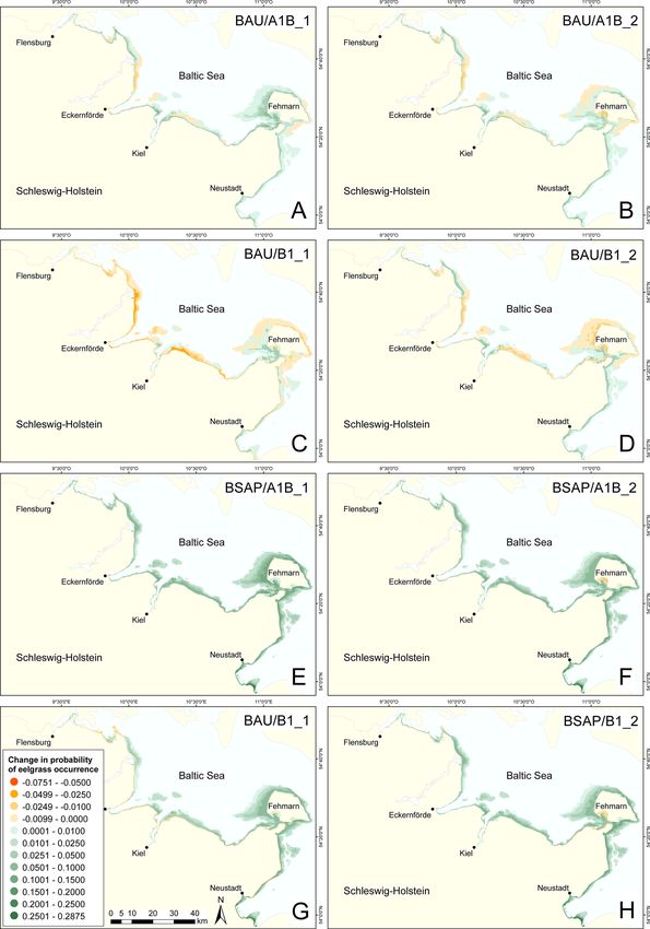
Ambio 2021, 50:400–412                                                                                                     401

improve water quality and clarity, foster sediment stability     Model approach and response variables
and thus enhance coastal protection, and bind and sequester
nutrients and carbon (Moore 2004; Ondiviela et al. 2014;         We applied the software GRASP (generalized regression
Duarte and Krause-Jensen 2017). Due to their ability to          analysis and spatial prediction, Lehmann et al. 2002)
accumulate and store organic carbon in the sediments over        within the statistics package R (R Development Core Team
millennial time scales, seagrass meadows are significant         2008) to calculate generalized additive models (Hastie and
‘‘blue carbon’’ sinks (Fourqurean et al. 2012). However,         Tibshirani 1990). GRASP allows for generating species
seagrass beds are facing significant anthropogenic threats       response curves showing the effect of the applied envi-
as a result of eutrophication and climate change (Duarte         ronmental gradients. The input data base of 7 150 geo-
et al. 2018). Currently, seagrasses are in decline, with         graphically referenced presence vs. absence records was
global annual losses of about 7% since 1990 (Waycott et al.      obtained from extensive eelgrass video transect mappings
2009) although losses in some European regions have come         in 2010 and 2011 (Schubert et al. 2015). The distribution
to a halt (de los Santos et al. 2019), prompting the question    model covers the study area from the shoreline down to
how meadows can be promoted to recover.                          12 m water depth (Fig. 1) with a grid size of 100 m,
   We here couple climate-forcing projections of sea state       comprising a total area of 828 km2. For each grid point the
and biogeochemical model projections of water turbidity          model calculated the probability of eelgrass occurrence
with species niche modeling to forecast the future spatial       (values ranging from 0 to 1). The balanced prevalence with
distribution of the eelgrass (Zostera marina) on local           the same numbers of presence and absence records allowed
scales. Input variables represent ecological key predictors,     for translating the probabilities of eelgrass occurrence
which were parameterized to the International System of          directly to probabilities of plant encounter (equivalent to
Units to simplify future projections. Our main objective         percent eelgrass coverage) without further modification
was to quantify Zostera marina’s spatial response to             (Liu et al. 2005). Water depths for model calculations were
nutrient mitigation efforts according to the BSAP reduction      derived from an array of diverse digital elevation models.
targets in combination with future climate change and            First, a digital bathymetric map based on airborne LiDAR
resulting sea state scenarios.                                   measurements (Light Detection and Ranging) from
                                                                 between 2014 and 2016 (1 m spatial resolution), delivered
                                                                 values for the shallowest coastal regions from 0 to 2.5 m.
MATERIALS AND METHODS                                            This data set and a digital shoreline produced from aerial
                                                                 orthographic photos taken in 2013 were provided by the
Study site                                                       State Agency for Coastal Protection, National Park and
                                                                 Marine Conservation Schleswig–Holstein (LKN.SH). In
The study region comprises the western part of the Baltic        places where no LiDAR depth data were available, we used
Sea coast in northern Germany (i.e., the federal state’s         interpolated sonar depth measurements of the Federal
Schleswig-Holstein eastern coastline). Relatively shallow        Maritime and Hydrographic Agency (BSH, Germany)
bays and one island (Fehmarn) characterize this region           between 1982 and 2004. This bathymetric layer covers
(Fig. 1).                                                        water depths from 1.0 to 34.0 m with a horizontal resolu-
   Due to prevailing westerly winds and the enclosed             tion of 10 to 50 m. Some still missing depth data, primarily
character of the coast, wave exposure is mostly slight and       in places deeper than 10 m, were taken from a third
significant wave heights rarely exceed 3 m (Petterson et al.     bathymetric map with 50 m spatial resolution, which was
2018). Shallow surface water salinity ranges from * 8            provided by the State Agency of Agriculture, Environment
to * 18 PSU depending on inflow events of fully saline           and Rural Areas Schleswig–Holstein.
water from the North Sea, as well as location and depth
(Franz et al. 2019). Water currents are weak overall except      Environmental predictors
for narrow fjords, when strong winds induce rapid sea-level
changes. The sea bottom primarily consists of sandy-to-          We designated light availability for eelgrass and wave-
muddy sediments, partly interspersed with boulders, cob-         generated water current at the bottom as the most important
bles, and gravel. Bedrock is absent throughout the study         environmental variables regulating the spatial distribution
area. Eelgrass is the dominant vegetation type along the         of eelgrass. While the environmental variable ‘‘salinity’’
coastline, where it inhabits water depths between 1 and 8 m      had been tested in earlier model runs based on the same set
(Schubert et al. 2015).                                          of eelgrass distribution input data (Schubert et al. 2015), it
                                                                 does not significantly increase the predictive power of the
                                                                 eelgrass model and was therefore excluded from the cur-
                                                                 rent model.

                                                     Ó The Author(s) 2020
                                                        www.kva.se/en                                               123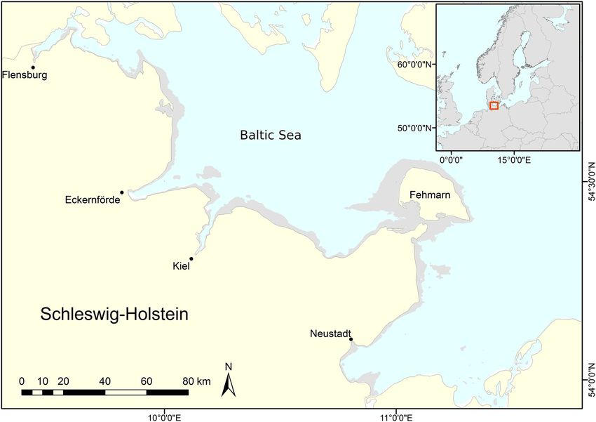
402                                                                                                            Ambio 2021, 50:400–412

Fig. 1 Baltic Sea coast of Schleswig-Holstein with the island of Fehmarn. Water depths \ 12 m are marked with gray color

Light availability                                                    according to Kirk (1994) nearly 6% of the incident light is
                                                                      reflected from the water, some overestimation ensues.
Photosynthetic photon flux density (PFD, lmol photons                    To obtain estimates for future changes of PFD in the
m-2 s-1) available for plant growth was calculated for a              context of nutrient discharge regulation measures, we ran
depth of 0.5 m above sea floor (roughly corresponding to              simulations with ERGOM-MOM. This model encloses the
the top of the eelgrass canopy) using Beer’s law                      whole Baltic Sea, but only data points at the study area
Iz = I0 9 e-k9z (Kirk 1994), where Iz denotes the irradiance          (with a grid resolution of 1 nautical mile) were used.
at water depth z, I0 the surface irradiance, and k the light          ERGOM-MOM incorporates the inorganic nutrients
attenuation coefficient. Mean monthly surface solar irra-             ammonium, nitrate, and phosphate, which enter the Baltic
diance was taken from the European Commission’s Pho-                  Sea via waterborne loads and atmospheric deposition, as
tovoltaic Geographical Information System PGIS (http://re.            well as three functional phytoplankton groups, and one
jrc.ec.europa.eu/pvgis/apps4/pvest.php?lang=de&map=                   bulk group of zooplankton and detritus (Neumann 2000).
europe), based on satellite measurements between 1998                 Light attenuation was calculated depending on phyto-
and 2011 (Huld et al. 2012). For simplicity, the surface              plankton and detritus concentrations (Friedland et al.
irradiance of a representative position in the model region           2012). Modeled Secchi depths were validated using
(54°280 5800 N, 10°210 3600 E) was used over the entire model         empirical observations obtained from the responsible
grid. Irradiance to PFD conversion was achieved by mul-               environmental authorities and institutions, i.e., the State
tiplying the solar irradiation (W m-2) with a factor of 4.15          Agency for Agriculture, Environment and Rural Areas.
(Morel and Smith 1974). The attenuation coefficient k was             Emission scenario A1B of the International Panel on Cli-
estimated from modeled Secchi depths (SD) taken from the              mate Change (IPCC) was used for the nutrient scenario
coupled biogeochemical and hydrological model ERGOM-                  assessment. The A1B scenario belongs to the A1 green-
MOM (Friedland et al. 2012). No attempt was made to                   house gas emission scenario family presented in the Spe-
account for variable surface roughness during different               cial Report of Emission Scenarios of the IPCC. The A1
wind situations, i.e., the model is based on plane water              family is characterized by rapid economic growth, a global
surface conditions (no wind-induced roughness). Since                 human population that peaks in mid-century and then
                                                                      gradually declines, a quick spread of new and efficient

                                                         Ó The Author(s) 2020
123                                                         www.kva.se/en
Ambio 2021, 50:400–412 403
technologies and a convergent world (globalization). The emission scenario) and B1 (global environmental emission
A1 scenario splits into three groups that describe alterna- scenario) (Nakićenović et al. 2000). Each of the two
tive directions of technological development with A1B emission scenarios were simulated twice, starting with
achieving a balance between fossil and non-fossil energy slightly different initial conditions (different years in the
sources (Nakićenović et al. 2000). past) and resulting in four possible model realizations. The
We ran two simulations with different nutrient load use of different realizations of the same emission scenario
scenarios. The first simulation assumes a full implemen- is a common approach used by the climate modeling
tation of the HELCOM nutrient input targets (BSAP sce- community to account for the internal variability of the
nario). The maximal allowable inputs given by the revised climate system. Consequently, four long-term wave pro-
Baltic Sea Action Plan (HELCOM 2013) are heeded from jections (two emission scenarios with two realizations
2021 on, after between 2012 and 2020 the nutrient loads each) were available as input for the eelgrass distribution
were reduced linearly. The second scenario (business as model (Dreier et al. 2014).
usual, BAU scenario) kept the nutrient loads from 2012
onwards constant on the level of the BSAP reference per- Reference state and modeling strategy
iod (1997–2003, HELCOM 2013). The baltic-wide differ-
ence between the two scenarios of the annual loads The species distribution model relates field observations of
amounts to approximately 118 kt nitrogen and 15 kt eelgrass occurrence to environmental variables. As eelgrass
phosphorus. mapping was performed in the summers of 2010 and 2011,
the latter year was taken to represent the reference status of
Hydrodynamic exposure to wave-generated orbital eelgrass distribution. The eelgrass distribution was
currents assumed to be in equilibrium with its environment with
presence in all suitable locations and absence in locations
Hydrodynamic exposure was represented by wave-gener- with unsuitable environmental conditions. The changes of
ated maximum orbital velocity (MOV) at the sea floor, the predictor variables are projected for future model sce-
which depends on the local sea state. It was calculated as a narios including two nutrient load scenarios and four future
function of simulated significant wave height (Hm0), mean wave scenarios. This implies that the same set of future
wave period (Tm02), and wave length (L) for intermediate wave data is applied once to each of the two nutrient load
water depths (z) according to linear wave theory. We scenarios. The eelgrass distribution model covers a time
applied the criterion that the maximum wave height (Hmax) period of 60 years (2007–2066). We specified twelve
cannot exceed the local water depth (d) at a certain point 5-year time slices (2007–2011 as the baseline, followed by
(Hmax/d \ 1). Based on the widely used assumption in 2012–2016, 2017–2021, etc., until 2062–2066) to model
coastal engineering praxis that Hm0 * H1/3, we calculated the future eelgrass distribution. Within each of these twelve
the maximum wave height as Hmax = 1.86 9 Hm0 (under intervals, a 5-year mean of the predictor variables was
the assumption of a Rayleigh distribution and N = 1 000 established. On the base of the twelve time intervals this
waves) and the maximum wave period as approach finally results in 92 model runs comprising four
THmax = 0.83 9 Hmax ? 3.17 (Schlamkow pers. comm.). models for the base line of eelgrass distribution
The necessary sea state data were derived from the (2007–2011) and eight model runs for each of the future
WBSSC (Western Baltic Sea State Climate Version) wave time intervals, accounting for 88 models.
model (Dreier et al. 2014). This model is based on the To visualize the changes in the future eelgrass occur-
third-generation spectral wave model SWAN (Simulating rence, we prepared maps showing the differences of the
Waves Nearshore, Booij et al. 1999). It includes (i) bathy- modeled probability of eelgrass occurrence between the
metric data of the western Baltic Sea with a horizontal reference period 2007–2011 and the 2061–2066 time
resolution of * 1 km, (ii) hourly wave spectra along the interval for each of the model scenarios (Table 1).
northern and eastern boundaries from the spectral wave To attribute spatial distribution patterns and areal
model WAM (The Wamdi Group 1988) for the whole changes to each of the predictor variables, we also pursued
Baltic Sea (Groll et al. 2017), and (iii) hourly wind data a ceteris paribus approach, by keeping one of the variables
from the regional climate model Cosmo-CLM (Lauten- (PFD resp. MOV) constant. Temporal trends of the total
schlager et al. 2009). The Cosmo-CLM model was forced eelgrass area were charted using 30-year running means.
from the global AOGCM ECHAM5/MPI-OM with
observed anthropogenic emissions (twentieth century run: Prediction accuracy
1961–2000) and with two of the future emission scenarios
used within IPCC-Assessment Report 4 (twenty-first cen- Model accuracy was ascertained in a five-fold cross-vali-
tury run: 2001–2100), namely A1B (global economic dation procedure by resampling, combined with threshold-
Ó The Author(s) 2020
www.kva.se/en 123404 Ambio 2021, 50:400–412
Table 1 Differences in 5-year means (± SD) of photon flux density (PFD), maximum orbital velocity (MOV), and probability of eelgrass
occurrence (PEO) between the 2007–2011 and the 2061–2066 time intervals as calculated with the eelgrass distribution model for the study area.
The BSAP scenario represents the complete implementation of the Baltic Sea Action Plan nutrient reduction targets. The BAU scenario
represents nutrient loads according to the BSAP reference period (1997–2003). The four MOV scenarios account for the greenhouse gas emission
scenarios A1B and B1 of the Intergovernmental Panel on Climate Change each in two random realizations. Finally, the eelgrass models combine
both approaches
Scenario Mean ± SD Min Max
-2 -1
PFD (lmol photons m s ) BSAP 8.2 ± 5.6 - 2.6 45.5
BAU 0.6 ± 2.2 - 10.2 9.4
MOV (m s-1) A1B_1 - 0.012 ± 0.012 - 0.66 0.001
A1B_2 - 0.008 ± 0.014 - 0.56 0.138
B1_1 0.007 ± 0.007 - 0.005 0.381
B1_2 - 0.0004 ± 0.011 - 0.377 0.241
PEO BSAP/A1B_1 0.045 ± 0.039 - 0.011 0.287
BSAP/A1B_2 0.040 ± 0.037 - 0.029 0.287
BSAP/B1_1 0.028 ± 0.032 - 0.06 0.238
BSAP/B1_2 0.036 ± 0.035 - 0.042 0.282
BAU/A1B_1 0.012 ± 0.017 - 0.065 0.109
BAU/A1B_2 0.008 ± 0.016 - 0.06 0.112
BAU/B1_1 - 0.003 ± 0.012 - 0.075 0.048
BAU/B1_2 0.003 ± 0.013 - 0.067 0.079
independent receiver-operating-characteristic analysis flattens at [ 1 m s-1, while water currents \ 0.4 m s-1 are
(ROC, Fielding and Bell 1997). For each of the five iter- indicative of eelgrass presence.
ations within the validation process a subset of the data was
withhold during model building and used as test data. Model scenarios
Calculating the area under the ROC curve (AUC) provides
a measure of the model’s discriminatory capacity. With The different model runs predict widely divergent future
AUC values ranging from 0.5 to 1.0, a value of 0.5 denotes eelgrass distribution patterns. Compared to the reference
no, 0.7 low, 0.7 to 0.8 acceptable, and 0.8 to 0.9 excellent period (2007–2011), the mean eelgrass distribution area
discriminative abilities (Hosmer and Lemeshow 2000). increases by 16.3 ± 2.9% (mean ± SD) in the Baltic Sea
Action Plan model scenarios (BSAP) until 2066, corre-
sponding to an overall areal increase of 30.1 ± 5.3 km2
RESULTS
Our eelgrass distribution model features acceptable predic-
tion accuracy with a mean five-fold cross-validated Area
Under Curve value of 0.77 ± 0.01 (mean ± SD) over all
emission scenarios. Photon flux density PFD and maximal
orbital water velocity MOV proved to be suitable environ-
mental variables for predicting eelgrass occurrence, with
57.2% and 42.7% contribution, respectively. The eelgrass
response curves show opposite curve characteristics across PFD MOV
the gradients of light and wave-induced water currents Fig. 2 Response of Zostera marina to PFD (Photon Flux Density,
(Fig. 2). lmol photons m-2 s-1 at 0.5 m above the sea floor) and MOV
Eelgrass response to increasing light intensities shows a (maximum orbital wave velocity, m s-1 at the sea floor). The range of
saturation-type response with a linear positive slope until both predictor variables is displayed on the x-axis while the y-axis
shows the probability of eelgrass occurrence (on a logit scale). The
200 lmol photons m-2 s-1 are attained. In contrast, eel- horizontal dashed line marks the probability of occurrence of 0.5.
grass distribution steeply decreases with increasing orbital Small ticks above the x-axis represent single observations; the semi
water movement. The response curve declines until it dashed lines indicate the 95% confidence interval limits around the
response curve
Ó The Author(s) 2020
123 www.kva.se/enAmbio 2021, 50:400–412 405
(mean ± SD) (Fig. 3e–h). Depending on the modeled wave Total eelgrass area
scenarios and on the selected time slice, increasing or
decreasing maximum orbital velocities either strengthens In contrast to business as usual, the overall eelgrass area
or weakens eelgrass expansion. expanded considerably under nutrient abatement as
The most significant increases in eelgrass occurrence of required by the Baltic Sea Action Plan (BSAP). Substantial
19.9% (36.6 km2), 17.7% (32.8 km2), and 15.6% increase will occur over the last 15 years with a time lag of
(28.8 km2) were found based on the BSAP scenario in about 30 years after the full implementation of the nutrient
combination with climate wave scenarios A1B_1, A1B_2, reduction targets in 2021 (Fig. 4). The variation within both
and B1_2, respectively (Fig. 3e–h), when nutrient reduc- nutrient reduction scenarios (BSAP and BAU) is exclu-
tion occurs along with decreasing wave energy (i.e., sively attributable to changes in MOV and therefore a
maximum orbital velocity, MOV values) (Table 1). Like- result of the random variability in the four realizations of
wise, but less prominent, an increase of 11.9% (22.3 km2) the emission scenarios.
was observed within the BSAP/B1_1 scenario (Fig. 3g)
when nutrient abatement coincides with increasing MOV Predicting eelgrass depth distribution
(Table 1).
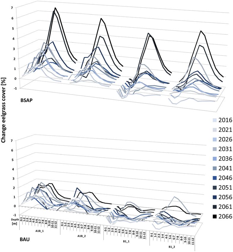
The overall changes in eelgrass occurrence under busi- The applied predictor variables modulate the eelgrass dis-
ness as usual range from - 1.3% in the B1_1 to ?1.1% in tribution differently in different depth zones. Improved
the B1_2 and from ?3.6% in the A1B_2 to ?5.3% in the light supply leads to increasing eelgrass predictions,
A1B_1 wave scenario until 2066 (Fig. 3c–a). Negative especially at greater depth, such that within the BSAP
impact of higher MOV (?3.9 ± 1.8% until 2066; models the probability of occurrence rises considerably
mean ± SD) on the overall eelgrass distribution is most between 4 and 8 m, with a maximum at 5 to 6 m (Fig. 5).
apparent in the B1_1 wave scenario (Fig. 3c), where the Conversely, high variation is caused by MOV in the dif-
total eelgrass coverage decreases by 2.5 km2. This scenario ferent climate wave scenarios at water depths \ 4 m.
is characterized by wide-ranging spatial variation for all of Below 8 m the variability decreases continuously to mini-
the open exposed coastlines as well as the shallow shel- mum levels at a lowest depth of 11–12 m (Fig. 5).
tered bays, but also for deeper eelgrass meadows. While
the overall effect on the predicted eelgrass occurrence is
comparably low in the BAU scenario in combination with DISCUSSION
the A1B_1, A1B_2, and B1_2 wave scenarios (Fig. 3a, b,
and d) the modeling results still indicate potential sensitive Our scenario modeling indicates that nutrient abatement
areas. These regions are sheltered areas such as the Orth according to the Baltic Sea Action Plan (BSAP scenario)
Bay in the southwest of the island of Fehmarn and Gelting enhances the occurrence of Z. marina along the Baltic
Bay eastwards of Flensburg, but also exposed sections of coast of northern Germany. Remarkably, the areal expan-
the outer coastal strip (Fig. 3). sion, which is expected as a benefit of nutrient reduction,
more than compensates potential areal loss from stormier
Ceteris paribus modeling conditions and higher wave energy under anticipated cli-
mate scenarios. Assuming the BSAP scenario enhanced
When keeping the maximum orbital velocity (MOV) con- light levels in the eelgrass meadows’ growing zone shift
stant until 2066, changes in photon flux density (PFD) the suitable habitat conditions to greater depth, which
cause the mean eelgrass distribution in the Baltic Sea induces a net increase of eelgrass coverage.
Action Plan scenario (BSAP) to increase by 15.1 ± 0.5% Hence, our results highlight the paramount significance
(mean ± SD), while being nearly unaffected under busi- of nutrient reduction measures to the recovery of threat-
ness as usual conditions (0.9 ± 0.05%; mean ± SD). If on ened and ecologically valuable eelgrass meadows. Further,
the other hand PFD is kept constant, the mean eelgrass they underline that the specified BSAP reduction targets
distribution is not changing significantly (1.2 ± 2.5%; suffice to initiate environmental improvement. Therefore,
mean ± SD), but the large confidence range indicates the implementation of the BSAP targets should be pursued
MOV to tip the scales to a positive or negative outcome. persistently, the more so as latest findings indicate that
Finally, changes in PFD contribute 93% to the total areal nutrient inputs into the Baltic Sea are on the rise again after
change in the BSAP scenarios, whereas changes in MOV a phase of conspicuous decline (Murray et al. 2019; Olesen
potentially contribute 83% to the variation. Conversely, et al. 2019).
MOV contributes 57% to the total eelgrass areal change in Assuming a business as usual (BAU) scenario, the
the BAU scenarios, whereas PFD contributes only 2% to ERGOM-MOM model projections suggest no significant
the variation. deterioration of the underwater light conditions for the
Ó The Author(s) 2020
www.kva.se/en 123406 Ambio 2021, 50:400–412
Fig. 3 Changes in probability of eelgrass occurrence at the Baltic Sea coast of Schleswig-Holstein until 2066. BAU represents the business as
usual nutrient regime, referring to constant nutrient loads on the level of the BSAP reference period (a–d) while BSAP represents the full
implementation of the Baltic Sea Action Plan nutrient reduction targets (e–h). Both regimes are combined with climate-related variation of wave
power according to the A1B and B1 greenhouse gas emission scenarios of the Intergovernmental Panel on Climate Change, each in two random
realizations
Ó The Author(s) 2020
123 www.kva.se/enAmbio 2021, 50:400–412 407
230
BAU/A1B_1
BAU/A1B_2
BAU/B1_1
220 BAU/B1_2
BSAP/A1B_1
BSAPA1B_2
BSAP/B1_1
Eelgrass area [km 2 ] BSAP/B1_2
210
200
190
180
0
2011 2016 2021 2026 2031 2036 2041 2046 2051 2056 2061 2066
Fig. 4 Modeled overall eelgrass area for the Baltic Sea coast of Schleswig-Holstein until 2066 as a function of nutrient reduction scenarios and
climate-related sea state conditions. Data points represent running means over 30 years. BSAP: Implementation of the Baltic Sea Action Plan
nutrient reduction targets. BAU: nutrient loads according to the BSAP reference period. A1B and B1 represent the greenhouse gas emission
scenarios according to the Intergovernmental Panel on Climate Change each in two random realizations
study region until 2066 (Table 1). Consequently, the eel- size of the overall distribution area. Within the B1_1 cli-
grass model indicates no substantial change of the overall mate scenario, however, the model runs indicate substantial
eelgrass coverage, which suggests that we are presently losses of shallow eelgrass meadows along the entire
looking at some kind of equilibrium distribution that will coastline across both nutrient regimes. Thus, more frequent
likely not further deteriorate. Like in most other regions of and more violent storm events in the future may weaken
the Baltic Sea, the eelgrass meadows of the German Baltic the eelgrass’ potential for coastal erosion control (Ondi-
Coast (Schleswig–Holstein) declined to nearly 50% of their viela et al. 2014).
historical distribution in the 1960s mainly as a result of The species distribution model reproduces the eco-
eutrophication effects (Boström et al. 2014; Schubert et al. physiological tenet that light determines the macrophytes’
2015). While some coastal regions still suffer losses lower depth distribution, while physical exposure restricts
without any signs of reaching equilibrium or trend reversal the upper depth limit (Krause-Jensen et al. 2003).
(Moksnes et al. 2018) recent studies reported that the rate Assuming the BSAP scenario and hence more translucent
of seagrass losses slowed down for most of the European water conditions, eelgrass distribution primarily increases
seagrass species and fast growing species even recovered in at the current lower depth limit of 4 to 8 m (Schubert et al.
some locations (de los Santos et al. 2019). Actual moni- 2015). In contrast, changes in wave energy, reflected in our
toring data for the Baltic Sea coast of Schleswig-Holstein chosen variable MOV, primarily affect eelgrass occurrence
confirm the same overall maximum depth limits of eelgrass in 1 to 2 m depth, which coincides with the current mini-
or even slightly increasing trends over the last 10 years mum depth distribution in the study area.
(Karez pers. com.), which supports the idea of a current Reassuringly, our modeling results closely match with
equilibrium distribution. These findings coincide with known ecophysiological data on eelgrass light require-
observations of Riemann et al. (2016) for Danish eelgrass ments (Lee et al. 2007) and tolerable water currents (Koch
meadows. 2001). The photon flux density (PFD) response curve
The variations in eelgrass distribution patterns do not indicates a positive correlation of eelgrass occurrence with
only result from changes in wave height, but also from light intensities (Fig. 2) and with levels above 150 lmol
changes in wave direction (Dreier et al. 2014). Maximum photons m-2 s-1 (corresponding to about 25% of the solar
orbital velocity (MOV) primarily affects the shallow dis- surface irradiation) contributing positively to model pre-
tribution limit of eelgrass with only minor impact on the dictions. This value fits into the range of eelgrass light
Ó The Author(s) 2020
www.kva.se/en 123408 Ambio 2021, 50:400–412
Fig. 5 Percentual changes in eelgrass coverage as a function of water depth dependent on nutrient reduction scenarios and climate-related wave
scenarios. BSAP: Implementation of the Baltic Sea Action Plan nutrient reduction targets. BAU: nutrient loads according to the BSAP reference
period (1997–2003). A1B and B1 represent greenhouse gas emission scenarios according to the Intergovernmental Panel on Climate Change
each in two random realizations
compensation points calculated for whole plants (Lee et al. m-2 s-1 (Fig. 2), in turn coinciding with eelgrass light
2007) and coincides with the minimum light requirement saturation points for photosynthesis that are calculated for
for eelgrass, which varies between 18 and 29% of the whole plants (Lee et al. 2007). The response curve for
surface irradiance (Krause-Jensen et al. 2011). The maximum orbital velocity indicates negative correlation
response curve for PFD flattens above 350 lmol photons with bottom water velocity, and the modeled habitat
Ó The Author(s) 2020
123 www.kva.se/enAmbio 2021, 50:400–412 409
characteristics for eelgrass are less suitable if maximal We disregarded some restrictions or physical constraints
water movement exceeds 0.4 m s-1. This threshold seems that might possibly limit eelgrass expansion (Kuusemäe
realistic for the study area. Generally, Z. marina can tol- et al. 2016), especially, we excluded salinity from the
erate maximum current velocities of up to 0.5 to 1.8 m s-1 current model because it did not significantly increase the
(Koch 2001). Fonseca and Kenworthy (1987), however, predictive power of the model as tested in previous model
reported 0.5 m s-1 as a critical limit for the persistence of runs (Schubert et al. 2015), which comes as no surprise as
Z. marina meadows. In contrast to the nutrient reduction Z. marina is well adapted to low salinity and tolerates large
scenario, the overall eelgrass area in the BAU scenario salinity variations (Boström et al. 2014). Salinity as a
remains nearly constant but shows an oscillating pattern. regulating factor for Z. marina distribution becomes
This wave-like pattern accounts for the interannual vari- important in estuaries, freshwater-influenced lagoons, and
ability, which leads in the 3D model to increased chloro- brackish seas (oligohaline\ 5 psu) where eelgrass is living
phyll concentrations and decreased Secchi depths around at the edge of its salinity tolerance, while in our area,
the year 2040. This increase is in agreement with previous salinity is never below 8 psu. We recommend, however,
studies, e.g., Friedland et al. (2012), who reported an including salinity to seagrass distribution models within
increase of summer chlorophyll-a in the western Baltic Sea areas where salinity is expected to reach the tolerance
due to climate change, even if nutrient inputs stay on recent levels of the respective seagrass species.
levels. The predicted overall eelgrass increases in the Another process that may be given more consideration is
nutrient reduction scenarios are not evenly distributed over the sediment-light feedback mechanism (van der Heide
the modeled time period. Our model indicates that the et al. 2011). Typically, dense seagrass meadows attenuate
nutrient abatement will improve eelgrass growth and water currents and stabilize sediments; thereby they pro-
abundance with a considerable delay of about 30 years. mote sedimentation and reduce resuspension of particles,
The time delay could be explained by the nutrient resi- which results in clearer water and more suitable growth
dence times in the Baltic Sea, as Radtke et al. (2012) conditions. At the moment, there is no stabilization feed-
estimated nutrients to stay at least 30 years in the Baltic back from eelgrass on the sediments included in the 3D-
Sea. But recovery times of submerged aquatic vegetation model (ERGOM-MOM), which was used to estimate the
after cessation of nutrient inputs often take even longer and future development of light attenuation. It is well known
may vary from several years to nearly a century that losses of seagrass, however, may trigger a regime shift
(McCrackin et al. 2016). Dispersal by seeds and rafting to a more turbid state characterized by wind-driven resus-
shoots to particular locations may not be efficient, and once pension of sediments that are no longer stabilized by eel-
first colonizers arrive, it may take some time until critical grass and therefore cause unsuitable light conditions for
threshold densities are exceeded that allow for continual eelgrass colonization (Maxwell et al. 2016). Regime shifts
growth of the colonizing patches (Olesen and Sand-Jensen to alternative stable states may prevent natural recovery of
1994). For temperate eelgrass meadows in Danish waters, seagrass and make restoration quite difficult (Moksnes
Riemann et al. (2016) reported a similar time delay of et al. 2018).
increasing depth limits after 25 year of consistent nutrient Biotic interactions may also be important environmental
mitigation measures. Light and water currents have been factors regulating the distribution of seagrasses (Nakaoka
identified as major factors most often regulating the sur- 2005). The loss of large predatory fish in the northern
vival and the depth distribution of seagrasses (de Boer Kattegat, for example, induced complex trophic cascades
2007). Therefore, we suggest the principal model approach affecting the survival of eelgrass due to light deficiency
to be directly applicable to other marine macrophyte spe- (Moksness et al. 2008; Casini et al. 2009). Including biotic
cies or in other regions of the world. Essential requirements interactions in addition to purely abiotic parameters that
for model setup, however, include extensive seagrass dis- determine seagrass distribution is a major challenge for
tribution data combined with local biogeochemical und future research (Dormann et al. 2018). Further, major
hydrodynamic future model projections. Importantly, pre- remaining gaps in our knowledge are in the field of effects
dictive variables of the spatial distribution model have to of ocean warming. Increasing frequencies of heatwaves
be parameterized in such a way that they can be coupled have shown to cause large mortality among eelgrass in the
simultaneously to a climate-forcing model and to a bio- western Baltic Sea (Reusch et al. 2005) and their effects
geochemical ecosystem model. can be exacerbated due to increased water turbidity and
The model calculates suitable habitat conditions (refer- anoxia (Moore and Jarvis 2008). We currently lack suffi-
ring to light and wave-induced water currents as most cient data to translate the expected rapid warming of Baltic
important variables) on the basis of field observations and Sea surface waters into eelgrass growth and distribution
translates future variations of these conditions to areal responses. Future sea level rise is another variable that
changes (expansion or retreat) of the eelgrass distribution. needs further work, as it would effectively increase the
Ó The Author(s) 2020
www.kva.se/en 123410 Ambio 2021, 50:400–412
actual bathymetric depth of up to 1 m, shifting the future REFERENCES
distribution of eelgrass nearer to the present shorelines and
requiring a shoreward distributional shift of some meadows Backer, H., J.M. Leppanen, A.C. Brusendorff, K. Forsius, M.
Stankiewicz, J. Mehtonen, M. Pyhala, M. Laamanen, et al.
occurring under very shallow slopes by hundreds of meters. 2010. HELCOM Baltic Sea Action Plan—a regional programme
of measures for the marine environment based on the Ecosystem
Approach. Marine Pollution Bulletin 60: 642–649.
CONCLUSION Booij, N., R.C. Ris, and L.H. Holthuijsen. 1999. A third-generation
wave model for coastal regions: 1. Model description and
validation. Journal of Geophysical Research: Oceans 104:
We combined species distribution modeling with an 7649–7666.
ecosystem nutrient model and a climate forced wave Boström, C., S. Baden, A. Bockelmann, K. Dromph, S. Fredriksen, C.
forecasting model, which allowed us to project the spatial Gustafsson, D. Krause-Jensen, T. Möller, et al. 2014. Distribu-
tion, structure and function of Nordic eelgrass (Zostera marina)
response of eelgrass to nutrient management measures in ecosystems: implications for coastal management and conserva-
combination with emerging climate change and associated tion. Aquatic Conservation: Marine and Freshwater Ecosystems
increase of wave energy. Our key result is that meeting 24: 410–434.
nutrient reduction targets of the HELCOM Baltic Sea Casini, M., J. Hjelm, J.-C. Molinero, J. Lövgren, M. Cardinale, V.
Bartolino, A. Belgrano, and G. Kornilovs. 2009. Trophic
Action Plan would allow eelgrass to expand considerably cascades promote threshold-like shifts in pelagic marine ecosys-
and mostly in the vicinity to already existing eelgrass tems. Proceedings of the National Academy of Sciences of the
occurrences. We therefore do not anticipate that over United States of America 106: 197–202.
decadal time scales dispersal limitation would delay Dormann, C.F., M. Bobrowski, D.M. Dehling, D.J. Harris, F. Hartig,
H. Lischke, M.D. Moretti, J. Pagel, et al. 2018. Biotic
recolonization much. The areal expansion and the interactions in species distribution modelling: 10 questions to
increasing expansion into depth are likely to improve the guide interpretation and avoid false conclusions. Global Ecology
ecological status of the German Baltic coastal water bodies and Biogeography 27: 1004–1016.
as required by the European Water Framework Directive Dreier, N., P. Fröhle, D. Salecker, C. Schlamkow, and Z. Xu. 2014.
The use of a regional climate- and wave model for the
(EC 2000), which aims to achieve a ‘‘good ecological assessment of changes of the future wave climate in the western
status’’ of the European surface waters. Baltic Sea. In Proceedings of the 34th international conference
Arguably, the exact projected distributional changes in on coastal engineering. Seoul, Korea, 15–20 June 2014.
eelgrass should not be taken at face value, but rather Duarte, C.M., and D. Krause-Jensen. 2017. Export from seagrass
meadows contributes to marine carbon sequestration. Frontiers
viewed as possible outcomes of divergent anticipated cli- in Marine Science 4: 13.
mate and ecosystem scenarios. The modeled expansion of Duarte, B., I. Martins, R. Rosa, A.R. Matos, M.Y. Roleda, T.B.H.
eelgrass under ongoing nutrient abatement in our study Reusch, A.H. Engelen, E.A. Serrão, et al. 2018. Climate change
nevertheless suggests that curbing nutrient input, though impacts on seagrass meadows and macroalgal forests: An
integrative perspective on acclimation and adaptation potential.
requiring considerable and growing effort in agricultural Frontiers in Marine Science 5: 190.
practices, will continue to pay off. EC. 2000. Directive 2000/60/EC of the European parliament and of
the council of 23 October 2000 establishing a framework for
Acknowledgements Open Access funding provided by Projekt community action in the field of water policy (Water framework
DEAL. This research was funded by the State Agency for Agriculture, directive). Official Journal of the European Communities L 327:
Environment and Rural Areas Schleswig-Holstein (LLUR). The 1–73.
LLUR (Hans Christian Reimers) and Agency for Coastal Defence, EC. 2008. Directive 2008/56/EC of the European parliament and of
National Park and Marine Conservation (Lutz Christiansen) kindly the council of 17 June 2008 establishing a framework for
provided the bathymetry data for the German Baltic Sea. We are community action in the field of marine environmental policy
grateful to the reviewers who provided valuable comments and con- (Marine strategy framework directive). Official Journal of the
structive criticism and helped to improve the manuscript. European Union L 164/19 2008.
de Boer, W.F. 2007. Seagrass-sediment interactions, positive feed-
Open Access This article is licensed under a Creative Commons backs and critical thresholds for occurrence: A review. Hydro-
Attribution 4.0 International License, which permits use, sharing, biologia 591: 5–24.
adaptation, distribution and reproduction in any medium or format, as de los Santos, C.B., D. Krause-Jensen, T. Alcoverro, N. Marba, C.M.
long as you give appropriate credit to the original author(s) and the Duarte, M.M. van Katwijk, M. Pérez, J. Romero, et al. 2019.
source, provide a link to the Creative Commons licence, and indicate Recent trend reversal for declining European seagrass meadows.
if changes were made. The images or other third party material in this Nature Communications 10: 3356.
article are included in the article’s Creative Commons licence, unless Fernandino, G., C.I. Elliff, and I.R. Silva. 2018. Ecosystem-based
indicated otherwise in a credit line to the material. If material is not management of coastal zones in face of climate change impacts:
included in the article’s Creative Commons licence and your intended Challenges and inequalities. Journal of Environmental Manage-
use is not permitted by statutory regulation or exceeds the permitted ment 215: 32–39.
use, you will need to obtain permission directly from the copyright Fielding, A.H., and J.F. Bell. 1997. A review of methods for the
holder. To view a copy of this licence, visit http://creativecommons. assessment of prediction errors in conservation presence/absence
org/licenses/by/4.0/. models. Environmental Conservation 24: 38–49.
Ó The Author(s) 2020
123 www.kva.se/enAmbio 2021, 50:400–412 411
Fonseca, M.S., and W.J. Kenworthy. 1987. Effects of current on Maxwell, P.S., J.S. Eklöf, M.M. van Katwijk, K.R. O’Brien, M. de la
photosynthesis and distribution of seagrass. Aquatic Botany 27: Torre-Castro, C. Boström, T.J. Bouma, D. Krause-Jensen, et al.
59–78. 2016. The fundamental role of ecological feedback mechanisms
Fourqurean, J.W., C.M. Duarte, H. Kennedy, N. Marbà, M. Holmer, for the adaptive management of seagrass ecosystems—a review.
M.A. Mateo, E.T. Apostolaki, G.A. Kendrick, et al. 2012. Biological Reviews 92: 1521–1538.
Seagrass ecosystems as a globally significant carbon stock. McCrackin, M.L., H.P. Jones, P.C. Jones, and D. Moreno-Mateos.
Nature Geoscience 5: 505–509. 2016. Recovery of lakes and coastal marine ecosystems from
Franz, M., C. Lieberum, G. Bock, and R. Karez. 2019. Environmental eutrophication: A global meta-analysis. Limnology and
parameters of shallow water habitats in the SW Baltic Sea. Earth Oceanography 62: 507–518.
System Science Data 11: 947–957. Moksnes, P.-O., M. Gullström, K. Tryman, and S. Baden. 2008.
Friedland, R., T. Neumann, and G. Schernewski. 2012. Climate Trophic cascades in a temperate seagrass community. Oikos 117:
change and the Baltic Sea Action Plan: Model simulations on the 763–777.
future of the western Baltic Sea. Journal of Marine Systems 105: Moksnes, P.-O., L. Eriander, E. Infantes, and M. Holmer. 2018. Local
175–186. regime shifts prevent natural recovery and restoration of lost
Fyhr, F., Å. Nilsson, and A. N. Sandman. 2013. A review of ocean eelgrass beds along the Swedish west coast. Estuaries and
zoning tools and species distribution modeling methods for Coasts 41: 1712–1731.
marine spatial planning. Aquabiota Water Research 27. Aqua- Moore, K.A. 2004. Influence of seagrasses on water quality in shallow
Biota Water Research, Stockholm, Sweden. regions of the lower Chesapeake Bay. Journal of Coastal
Groll, N., I. Grabemann, B. Hünicke, and M. Meese. 2017. Baltic Sea Research 10045: 162–178.
wave conditions under climate change scenarios. Boreal Envi- Moore, K.A., and J.C. Jarvis. 2008. Environmental factors affecting
ronment Research 22: 1–12. recent summertime eelgrass diebacks in the Lower Chesapeake
Hastie, T., and R. Tibshirani. 1990. Generalized additive models. Bay: Implications for long-term persistence. Journal of Coastal
London, UK: Chapman and Hall/CRC Press. Research 10055: 135–147.
HELCOM. 2007. Baltic Sea Action Plan (BSAP). HELCOM Morel, A., and R.C. Smith. 1974. Relation between total quanta and
Ministerial Meeting. Adopted in Krakow, Poland, 15 November total energy for aquatic photosynthesis. Limnology and
2007. http://www.helcom.fi/stc/files/BSAP/BSAP_Final.pdf. Oceanography 19: 591–600.
HELCOM, 2013. HELCOM Copenhagen Ministerial Declaration: Murray, C.J., B. Müller-Karulis, J. Carstensen, D.J. Conley, B.G.
Taking further action to implement the Baltic Sea Action Plan - Gustafsson, and J.H. Andersen. 2019. Past, Present and Future
reaching a good environmental status for a healthy Baltic Sea. Eutrophication Status of the Baltic Sea. Frontiers of Marine
Copenhagen, Denmark. HELCOM Declaration. Science 6: 2.
Hosmer, D.W., and S. Lemeshow. 2000. Applied logistic regression. Nakaoka, M. 2005. Plant-animal interactions in seagrass beds:
New York: Wiley. Ongoing and future challenges for understanding population
Huld, T., R. Muller, and A. Gambardella. 2012. A new solar radiation and community dynamics. Population Ecology 47: 167–177.
database for estimating PV performance in Europe and Africa. Nakićenović, N., J. Alcamo, G. Davis, B. de Vries, J. Fenhann, S.
Solar Energy 86: 1803–1815. Gaffin, K. Gregory, A. Grübler, et al. 2000. Emissions scenarios:
Kirk, J.T. 1994. Light and photosynthesis in aquatic ecosystems. A special report of working group III of the Intergovernmental
Cambridge: Cambridge University Press. Panels on Climate Change. Cambridge: Cambridge University
Koch, E.M. 2001. Beyond light: Physical, geological, and geochem- Press.
ical parameters as possible submersed aquatic vegetation habitat Neumann, T. 2000. Towards a 3D-ecosystem model of the Baltic Sea.
requirements. Estuaries 24: 1–17. Journal of Marine Systems 25: 405–419.
Krause-Jensen, D., M.F. Pedersen, and C. Jensen. 2003. Regulation of Nordlund, L.M., E.W. Koch, E.B. Barbier, and J.C. Creed. 2016.
eelgrass (Zostera marina) cover along depth gradients in Danish Seagrass ecosystem services and their variability across genera
coastal waters. Estuaries 26: 866–877. and geographical regions. PLoS ONE 11: 23.
Krause-Jensen, D., J. Carstensen, S.L. Nielsen, T. Dalsgaard, P.B. Olesen, B., and K. Sand-Jensen. 1994. Patch dynamics of eelgrass
Christensen, H. Fossing, and M.B. Rasmussen. 2011. Sea bottom Zostera marina. Marine Ecology Progress Series 106: 147–156.
characteristics affect depth limits of eelgrass Zostera marina. Olesen, J.E., C.D. Børgesen, F. Hashemi, M. Jabloun, D. Bar-
Marine Ecology Progress Series 425: 91–102. Michalczyk, P. Wachniew, A.J. Zurek, A. Bartosova, et al. 2019.
Kuusemäe, K., E.K. Rasmussen, P. Canal-Vergés, and M.R. Flindt. Nitrate leaching losses from two Baltic Sea catchments under
2016. Modelling stressors on the eelgrass recovery process in scenarios of changes in land use, land management and climate.
two Danish estuaries. Ecological Modelling 333: 11–42. Ambio 48: 1252–1263.
Lautenschlager, M., K. Keuler, C. Wunram, E. Keup-Thiel, M. Ondiviela, B., I.J. Losada, J.L. Lara, M. Maza, C. Galvan, T.J.
Schubert, A. Will, B. Rockel, and U. Boehm. 2009. Climate Bouma, and J. van Belzen. 2014. The role of seagrasses in
Simulation with COSMO-CLM, Climate of the 20th Century coastal protection in a changing climate. Coastal Engineering
Run No. 1-3, Scenario A1B Run NO. 1-2, Scenario B1 Run No. 87: 158–168.
1-2, Data Stream 3: European Region. MPI-M/MaD, World Data Petterson, H., K. Ola, and T. Brüning. 2018. Wave climate in the
Centre for Climate. Baltic Sea in 2017. HELCOM Baltic Sea Environment Fact
Lee, K.S., S.R. Park, and Y.K. Kim. 2007. Effects of irradiance, Sheets. Online. http://www.helcom.fi/baltic-sea-trends/
temperature, and nutrients on growth dynamics of seagrasses: A environment-fact-sheets/. Accessed 30 Aug 2019.
review. Journal of Experimental Marine Biology and Ecology Radtke, H., T. Neumann, M. Voss, and W. Fennel. 2012. Modeling
350: 144–175. pathways of riverine nitrogen and phosphorus in the Baltic Sea.
Lehmann, A., J.M. Overton, and J.R. Leathwick. 2002. GRASP: Journal of Ocean Research 117: C09024.
generalized regression analysis and spatial prediction. Ecolog- Rabalais, N.N., R.E. Turner, R.J. Dı́az, and D. Justić. 2009. Global
ical Modeling 157: 189–207. change and eutrophication of coastal waters. ICES Journal of
Liu, C., P.M. Berry, T.P. Dawson, and R.G. Pearson. 2005. Selecting Marine Science 66: 1528–1537.
thresholds of occurrence in the prediction of species distribu-
tions. Ecography 28: 385–393.
Ó The Author(s) 2020
www.kva.se/en 123412 Ambio 2021, 50:400–412
R Development Core Team. 2008. R: A language and environment Christian Schlamkow is a post researcher of the Coastal Engineering
for statistical computing. Vienna: R Foundation for Statistical Group of the University of Rostock. He is now working at the Ros-
Computing. tock Freight and Fishery Harbour.
Reusch, T.B.H., A. Ehlers, A. Hämmerli, and B. Worm. 2005. Address: Rostocker Fracht- und Fischereihafen GmbH, Fischerweg
Ecosystem recovery after climatic extremes enhanced by geno- 408, 18069 Rostock, Germany.
typic diversity. Proceedings of the National Academy of Sciences e-mail: christian.schlamkow@rfh.de
of the United States of America 102: 2826–2831.
Riemann, B., J. Carstensen, K. Dahl, H. Fossing, J.W. Hansen, H.H. René Friedland is senior scientist at IOW/Baltic Sea Research
Jakobsen, A.B. Josefson, D. Krause-Jensen, et al. 2016. Recov- Institute for Baltic Sea Research and has been working on the edge on
ery of Danish coastal ecosystems after reductions in nutrient ecosystem modeling, water quality, European legislations, and
loading: A holistic ecosystem approach. Estuaries and Coasts eutrophication abatement.
39: 82–97. Address: Leibniz-Institute for Baltic Sea Research Warnemünde,
Schubert, P.R., W. Hukriede, R. Karez, and T.B.H. Reusch. 2015. Seestraße 15, 18119 Rostock, Germany.
Mapping and modeling eelgrass Zostera marina distribution in e-mail: rene.friedland@io-warnemuende.de
the western Baltic Sea. Marine Ecology Progress Series 522:
79–95. Norman Dreier is a researcher at Hamburg University of Technology
van der Heide, T., E.H. van Nes, M.M. van Katwijk, H. Olff, and (TUHH). His research interests include the effects of climate change
A.J.P. Smolders. 2011. Positive feedbacks in seagrass ecosys- on waves and wave loads on coastal protection structures.
tems—Evidence from large-scale empirical data. PLoS ONE 6: Address: Institute of River and Coastal Engineering, Hamburg
e16504. University of Technology, Denickestr. 22, 21073 Hamburg, Germany.
WAMDI Group. 1988. The WAM Model-A Third Generation Ocean e-mail: norman.dreier@tuhh.de
Wave Prediction Model. Journal of Physical Oceanography 18:
1775–1810. Philipp R. Schubert is a doctoral researcher at the GEOMAR
Waycott, M., C.M. Duarte, T.J.B. Carruthers, R.J. Orth, W.C. Helmholtz Centre for Ocean Research Kiel. His thesis research con-
Dennison, S. Olyarnik, A. Calladine, J.W. Fourqurean, et al. centrates on anthropogenic impacts on seagrass habitats in the Baltic
2009. Accelerating loss of seagrasses across the globe threatens Sea both on local and regional scales.
coastal ecosystems. Proceedings of the National Academy of Address: GEOMAR Helmholtz Centre for Ocean Research Kiel,
Sciences of the United States of America 106: 12377–12381. Marine Evolutionary Ecology, Düsternbrooker Weg 20, 24105 Kiel,
Young, I.R., and A. Ribal. 2019. Multiplatform evaluation of global Germany.
trends in wind speed and wave height. Science 364: 548–552. e-mail: pschubert@geomar.de
Publisher’s Note Springer Nature remains neutral with regard to Rolf Karez is a scientific employee at EPA LLUR in Schleswig-
jurisdictional claims in published maps and institutional affiliations. Holstein. Here he is responsible for the monitoring of marine
macrophytes as implementation of EU directives.
Address: State Agency for Agriculture, Environment and Rural Areas
AUTHOR BIOGRAPHIES Schleswig-Holstein (LLUR), Hamburger Chaussee 25, 24220 Flint-
Ivo C. Bobsien (&) is a researcher at the GEOMAR Helmholtz bek, Germany.
Centre for Ocean Research Kiel. His research interests include the e-mail: rolf.karez@llur.landsh.de
ecology of marine macrophytes with emphasis on trophic interactions
in seagrass beds. Thorsten B. H. Reusch is a professor for Marine Evolutionary
Address: GEOMAR Helmholtz Centre for Ocean Research Kiel, Ecology and coordinates the research division Marine Ecology at the
Marine Evolutionary Ecology, Düsternbrooker Weg 20, 24105 Kiel, GEOMAR Helmholtz Centre for Ocean Research Kiel. He is inter-
Germany. ested in the ecological and evolutionary effects of global change,
e-mail: ibobsien@geomar.de which he studies in different species ranging from phytoplankton to
fish and marine coastal vegetation.
Wolfgang Hukriede is a freelance computer enthusiast with a special Address: GEOMAR Helmholtz Centre for Ocean Research Kiel,
interest in ecological research. Marine Evolutionary Ecology, Düsternbrooker Weg 20, 24105 Kiel,
Address: GEOMAR Helmholtz Centre for Ocean Research Kiel, Germany.
Marine Evolutionary Ecology, Düsternbrooker Weg 20, 24105 Kiel, e-mail: treusch@geomar.de
Germany.
e-mail: whukriede@geomar.de
Ó The Author(s) 2020
123 www.kva.se/enYou can also read