Multi-Channel Auto-Calibration for the Atmospheric Imaging Assembly using Machine Learning - University of ...
←
→
Page content transcription
If your browser does not render page correctly, please read the page content below
Astronomy & Astrophysics manuscript no. main                                                                                        ©ESO 2021
                                              January 8, 2021

                                                     Multi-Channel Auto-Calibration for the Atmospheric Imaging
                                                                 Assembly using Machine Learning
                                                  Luiz F. G. dos Santos1, 2 , Souvik Bose3, 4 , Valentina Salvatelli5, 6 , Brad Neuberg5, 6 , Mark C. M. Cheung7 , Miho
                                                                  Janvier8 , Meng Jin6, 7 , Yarin Gal9 , Paul Boerner7 , and Atılım Güneş Baydı̇n10, 11

                                                     1
                                                         Heliophysics Science Division, NASA, Goddard Space Flight Center, Greenbelt, MD 20771, USA
                                                     2
                                                         The Catholic University of America, Washington, DC 20064, USA
                                                     3
                                                         Rosseland Center for Solar Physics, University of Oslo,P.O. Box 1029 Blindern, NO-0315 Oslo, Norway
                                                     4
                                                         Institute of Theoretical Astrophysics, University of Oslo,P.O. Box 1029 Blindern, NO-0315 Oslo, Norway
                                                     5
                                                         Frontier Development Lab, Mountain View, CA 94043, USA
                                                     6
                                                         SETI Institute, Mountain View, CA 94043, USA
arXiv:2012.14023v2 [astro-ph.SR] 6 Jan 2021

                                                     7
                                                         Lockheed Martin Solar & Astrophysics Laboratory (LMSAL), Palo Alto, CA 94304, USA
                                                     8
                                                         Université Paris-Saclay, CNRS, Institut d’astrophysique spatiale, Orsay, France
                                                     9
                                                         OATML, Department of Computer Science, University of Oxford, Oxford OX1 3QD, UK
                                                    10
                                                         Department of Computer Science, University of Oxford, Oxford OX1 3QD, UK
                                                    11
                                                         Department of Engineering Science, University of Oxford, Oxford OX1 3PJ, UK

                                                   Received 2 December 2020 / Accepted – – —-

                                                                                                                ABSTRACT

                                                   Context. Solar activity plays a quintessential role in influencing the interplanetary medium and space-weather around Earth. Remote
                                                   sensing instruments on-board heliophysics space missions provide a pool of information about the Sun’s activity, via the measure-
                                                   ment of its magnetic field and the emission of light from the multi-layered, multi-thermal, and dynamic solar atmosphere. Extreme
                                                   UV (EUV) wavelength observations from space help in understanding the subtleties of the outer layers of the Sun, namely the chro-
                                                   mosphere and the corona. Unfortunately, such instruments, like the Atmospheric Imaging Assembly (AIA) on-board NASA’s Solar
                                                   Dynamics Observatory (SDO), suffer from time-dependent degradation that reduces their sensitivity. Current state-of-the-art calibra-
                                                   tion techniques rely on sounding rocket flights to maintain absolute calibration, which are infrequent, complex, and limited to a single
                                                   vantage point.
                                                   Aims. We aim to develop a novel method based on machine learning (ML) that exploits spatial patterns on the solar surface across
                                                   multi-wavelength observations to auto-calibrate the instrument degradation.
                                                   Methods. We establish two convolutional neural network (CNN) architectures that take either single-channel or multi-channel input
                                                   and train the models using the SDOML dataset. The dataset is further augmented by randomly degrading images at each epoch with
                                                   the training dataset spanning non-overlapping months with the test dataset. We also develop a non-ML baseline model to assess the
                                                   gain of the CNN models. With the best trained models, we reconstruct the AIA multi-channel degradation curves of 2010–2020 and
                                                   compare them with the sounding-rocket based degradation curves.
                                                   Results. Our results indicate that the CNN-based models significantly outperform the non-ML baseline model in calibrating instru-
                                                   ment degradation. Moreover, multi-channel CNN outperforms the single-channel CNN, which suggests the importance of cross-
                                                   channel relations between different EUV channels for recovering the degradation profiles. The CNN-based models reproduce the
                                                   degradation corrections derived from the sounding rocket cross-calibration measurements within the experimental measurement un-
                                                   certainty, indicating that it performs equally well when compared with the current techniques.
                                                   Conclusions. Our approach establishes the framework for a novel technique based on CNNs to calibrate EUV instruments. We
                                                   envision that this technique can be adapted to other imaging or spectral instruments operating at other wavelengths.
                                                   Key words. Sun: activity, UV radiation, and general - Techniques: image processing - Methods: data analysis - telescopes

                                              1. Introduction                                                           monitor the Sun, its extended atmosphere, space environments
                                                                                                                        around Earth and other planets of the solar system (Clarke 2016).
                                              Solar activity plays a significant role in influencing the inter-         One of the flagship missions of HSO is the Solar Dynamics Ob-
                                              planetary medium and space weather around Earth and all the               servatory (SDO, Pesnell et al. 2012). Launched in 2010, SDO
                                              other planets of the solar system (Schwenn 2006). Remote-                 has been instrumental in monitoring the Sun’s activity, and pro-
                                              sensing instruments on-board heliophysics missions can provide            viding a high volume of valuable scientific data every day with a
                                              a wealth of information on the Sun’s activity, primarily via cap-         high temporal and spatial resolution. It has three instruments on-
                                              turing the emission of light from the multi-layered solar atmo-           board: the Atmospheric Imaging Assembly (AIA, Lemen et al.
                                              sphere, thereby leading to the inference of various physical quan-        2012), which records high spatial and temporal resolution im-
                                              tities such as magnetic fields, plasma velocities, temperature and        ages of the Sun in the ultraviolet (UV) and extreme UV (EUV);
                                              emission measure, to name a few.                                          the Helioseismic & Magnetic Imager (HMI, Schou et al. 2012),
                                                   NASA currently manages the Heliophysics System Observa-              that provides maps of the photospheric magnetic field, solar sur-
                                              tory (HSO), which consists of a group of satellites that constantly
                                                                                                                                                                   Article number, page 1 of 12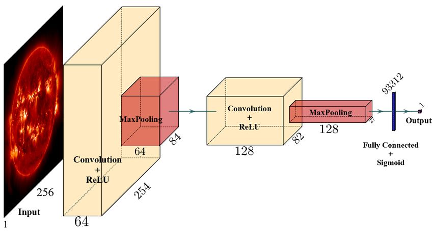
A&A proofs: manuscript no. main

                    094 Å           131 Å            171 Å                 193 Å               211 Å              304 Å               335 Å
May 13th, 2010
August 31st, 2019

     Fig. 1. Set of images to exemplify how degradation affects the AIA channels. The two sets are composed of seven images from different EUV
     channels. From left to right: AIA 94 Å, AIA 131 Å, AIA 304 Å, AIA 335 Å, AIA 171 Å, AIA 193 Å, and AIA 211 Å. The top row corresponds
     to images from May 13th , 2010 and the bottom row shows images from August 31 st , 2019, with no degradation correction. The 304 Å channel
     images are in log-scale due the severe degradation.

     face velocity and continuum filtergrams; and the EUV Variabil-                In general, first-principle models predicting the sensitivity
     ity Experiment (EVE, Woods et al. 2012), which measures the              degradation as functions of time and wavelength are not suffi-
     solar EUV spectral irradiance.                                           ciently well-constrained for maintaining the scientific calibra-
         Over the past decade, SDO has played a central role in ad-           tion of such instruments. To circumvent this problem, instru-
     vancing our understanding of the fundamental plasma processes            ment scientists have traditionally relied on empirical techniques,
     governing the Sun and space weather. This success can mainly             such as considering sources with known fluxes, the so-called
     be attributed to its open-data policy and a consistent high data-        "standard candles". However no standard candles exist on the
     rate of approximately two terabytes of scientific data per day.          solar atmosphere at these wavelengths since the solar corona is
     The large volume of data accumulated over the past decade (over          continuously driven and structured by evolving magnetic fields
     12 petabytes) provides a fertile ground to develop and apply             which caused localized and intermittent heating. This causes
     novel machine learning (ML) based data processing methods.               even the quiet Sun brightness in the EUV channels to vary signif-
     Recent studies, such as, predicting solar flares from HMI vector         icantly depending on the configuration of the small-scale mag-
     magnetic fields (Bobra & Couvidat 2015), creating high-fidelity          netic fields (Shakeri et al. 2015, and the references therein). On
     virtual observations of the solar corona (Salvatelli et al. 2019 &       the one hand, the Sun may not be bright enough to appear in
     Cheung et al. 2019), forecasting far side magnetograms from the          the hotter EUV channels such as AIA 94 Å . On the other hand,
     Solar Terrestrial Relations Observatory (STEREO, Kaiser et al.           active regions (ARs) have EUV fluxes that can vary by several
     2008) EUV images (Kim et al. 2019), super-resolution of mag-             orders of magnitude depending on whether it is in an emerging, a
     netograms (Jungbluth et al. 2019), and mapping EUV images                flaring or a decaying state. Moreover, the brightness depends on
     from AIA to spectral irradiance measurements (Szenicer et al.            the complexity of the AR’s magnetic field (van Driel-Gesztelyi
     2019), have demonstrated the immense potential of ML appli-              & Green 2015). Finally, ARs in the solar corona can evolve on
     cations in solar and heliophysics. In this paper, we leverage the        the time scales ranging from a few minutes to several hours, lead-
     availability of such high quality continuous observations from           ing to obvious difficulties in obtaining a standard flux for the
     SDO and apply ML techniques to address the instrument cali-              purpose of calibration.
     bration problem.                                                             Current state-of-the-art methods to compensate for this
         One of the crucial issues that limit the diagnostic capabili-        degradation rely on cross-calibration between AIA and EVE
     ties of SDO-AIA mission is the degradation of sensitivity over           instruments. The calibrated measurement of the full-disk solar
     time. Sample images from the seven AIA EUV channels in Fig. 1            spectral irradiance from EVE is passed through the AIA wave-
     show an example of such a deterioration. The top row shows the           length (filter) response function, to predict the integrated AIA
     images observed during the early days of the mission, from 13            signal over the full field of view. Later, the predicted band ir-
     May 2010, and the bottom row shows the corresponding images              radiance is compared with the actual AIA observations (Boerner
     observed more recently on 31 August 2019, scaled within the              et al. 2014). The absolute calibration of SDO-EVE is maintained
     same intensity range. It is clear that the images in the bottom          through periodic sounding rocket experiments (Wieman et al.
     row appear to be significantly dimmer compared to their top row          2016) that use a near-replica of the instrument on-board SDO
     counterparts. In some channels, especially 304 Å and 335 Å the           to gather a calibrated observation spanning the short interval of
     effect is pronounced.                                                    the suborbital flight (lasting a few minutes). A comparison of
                                                                              the sounding rocket observation with the satellite instrument ob-
         The dimming effect observed among the channels is due
                                                                              servation provides an updated calibration, revealing long-term
     to the temporal degradation of that EUV instruments in space
                                                                              trends in the sensitivities of EVE and, thus, of AIA.
     that is also known to diminish the overall instrument sensitivity
     with time (e.g., BenMoussa et al. 2013). The possible causes in-             Sounding rockets are undoubtedly crucial; however, the
     clude either the out-gassing of organic materials in the telescope       sparse temporal coverage (there are flights roughly every 2
     structure, which may deposit on the optical elements (Jiao et al.        years), and the complexities of inter-calibration are also potential
     2019), or the decrease in detector sensitivity due to exposure to        sources of uncertainty in the inter-instrument calibration. More-
     EUV radiation from the Sun.                                              over, the inter-calibration analysis has long latencies, of months
     Article number, page 2 of 12
Luiz F. G. dos Santos et al.: Multi-Channel Auto-Calibration for the Atmospheric Imaging Assembly using Machine Learning
and sometimes years, between the flights and when the calibra- in pixel brightness are directly related with the state of the Sun
tion can be updated, due to data analysis of the obtained data rather than instrument performance.
during the flight; also this kind of calibrations are limited to ob- In this paper, we applied a few additional pre-processing
servations from Earth, and thus cannot easily be used to calibrate steps. First, we downsampled the SDOML dataset to 256 × 256
missions in deep space (e.g., STEREO). pixels from 512 × 512 pixels. We established that 256 × 256
In this paper, we focus on automating the correction of the is a sufficient resolution for the predictive task of interest (in-
sensitivity degradation of different AIA wavebands by using ex- ference of a single coefficient) and the reduced size enabled a
clusively AIA information and adopting a deep neural network quicker processing and a more efficient use of the computational
(DNN, Goodfellow et al. 2016) approach, which exploits the resources. Secondly, we masked the off-limb signal (r > R ) to
spatial patterns and cross-spectral correlations among the ob- avoid possible contamination due to the telescope vignetting. Fi-
served solar features in multi-wavelength observations of AIA. nally, we re-scaled the brightness intensity of each AIA channel
We compare our approach with a non-ML method motivated by by dividing the image intensity by a channel-wise constant fac-
solar physics heuristics, which we call the baseline model. We tor. These factors represent the approximate average AIA data
evaluate the predicted degradation curves with the ones obtained counts in each channel and across the period from 2011 to 2018
through the sounding rocket cross-calibration described above. (derived from Galvez et al. 2019), and this re-scaling is imple-
To the best of our knowledge this is the first attempt to develop mented to set the mean pixel values close to unity in order to
a calibration method of this kind.1 We believe that the approach improve the numerical stability and the training convergence of
developed in this work could potentially remove a major imped- the CNN. Data normalization such as this is standard practice
iment to developing future HSO missions that can deliver solar in NNs (Goodfellow et al. 2016). The specific values for each
observations from different vantage points beyond Earth’s orbit. channel are reported in Appendix A.
The paper is structured as follows: in Section 2, we present
and describe our dataset. In Section 3 we illustrate the technique
and how it has been developed. Namely, in § 3.1 we state the 3. Methodology
hypothesis and propose a formulation of the problem, in § 3.2 3.1. Formulation of the problem
we present the CNN models, in § 3.3 we describe the training
process and the evaluation, in § 3.4 we probe the multi-channel It is known that some bright structures in the Sun are observed
relationship and in § 3.5 we reconstruct the temporal degrada- across different wavelengths. Figure 2 shows a good example
tion curve. Furthermore, in Section 4 we present the baseline, from 07 April 2015 of a bright structure in the center of all seven
followed by Section 5 where we present and discuss the results. EUV channels from AIA. Based on this cross-channel struc-
The concluding remarks are in Section 6. ture, we establish an hypothesis divided in two parts. First is
that there is a relationship between the morphological features
and the brightness of solar structures in a single channel (e.g.,
2. Data description and pre-processing typically, dense and hot loops over ARs). Second is that such a
We use for this study the pre-processed SDO-AIA dataset from relationship between the morphological features and the bright-
Galvez et al. (2019, hereafter referred to as SDOML). This ness of solar structures can be found across multiple channels of
dataset is ML-ready to be used for any kind of application re- AIA. We hypothesize that both these relationships can be used
lated to the AIA and HMI data and it consists of a subset of the to estimate the dimming factors and that a deep learning model
original SDO data ranging from 2010 to 2018. It comprises of can automatically learn these inter- and cross-channel patterns
the 7 EUV channels, 2 UV channels from AIA and vector mag- and exploit them for accurately predicting the dimming factor of
netograms from HMI. The data from the two SDO instruments each channel.
are temporally aligned, with cadences chosen to be 6 minutes To test our hypothesis we consider a vector C = {Ci , i ∈
for AIA (instead of the original 12 seconds) and EVE, and 12 [1, ..., n]} of multi-channel, synchronous SDO/AIA images,
minutes for HMI. The full disk images are downsampled from where Ci denotes the i-th channel image in the vector, and a
4096 × 4096 to 512 × 512 pixels and have identical spatial sam- vector α = {αi , i ∈ [1, ..., n]}, where αi is the dimming factor in-
pling of ∼ 400. 8 per pixel. dependently sampled from the continuous uniform distribution
In SDOML the AIA images have been compensated for the between [0.01, 1.0]. We choose an upper bound value of αi = 1,
exposure time and corrected for instrumental degradation over since we only consider dimming of the images and not enhance-
time using piecewise-linear fits to the V8 corrections released by ments. Further we create a corresponding vector of dimmed im-
the AIA team in November 2017.2 These corrections are based ages as D = {αiCi , i ∈ [1, ..., n]}, where D is the corresponding
on cross-calibration with SDO-EVE, where the EVE calibration dimmed vector. It is also to be noted that the dimming factors αi
is maintained by periodic sounding rocket under flights (includ- are applied uniformly per channel and are not spatially depen-
ing, in the case of the V8 corrections, a flight in 1 June 2016). dent. The spatial dependence of the degradation is assumed to
Consequently, the resulting dataset offers images where changes be accounted for by regularly updated flat-field corrections ap-
plied to AIA images. Our goal in this paper is to find a deep
1
We presented an early-stage result of this work as an extended ab- learning model M : D → α that retrieves the vector of multi-
stract at the NeurIPS workshop on ML and Physical Sciences 2019 channel dimming factors α from the observed SDO-AIA vector
(which has no formal proceedings) (NeurIPS 2019, Neuberg et al. D.
2019) where we described some preliminary results in this direction.
In this paper we extend the abstract with full analyses and discussion
of several important issues, such as the performance on the real degra- 3.2. Convolutional Neural Network Model
dation curve and the limitations of the presented models, that are both
crucial to evaluate the applicability of this ML based technique. Deep learning is a very active sub-field of machine learning
2
Available at https://aiapy.readthedocs.io/en/stable/ that focuses on specific models called deep neural networks
generated/gallery/instrument_degradation.html# (DNNs). A DNN is a composition of multiple layers of linear
sphx-glr-generated-gallery-instrument-degradation-py transformations and non-linear element-wise functions (Good-
Article number, page 3 of 12A&A proofs: manuscript no. main
AIA 94 AIA 131 AIA 171 AIA 193 AIA 211 AIA 304 AIA 335
0.0" 2015-04-07T22:32:49.120
Solar Y (arcsec)
-50.0"
-100.0"
-150.0"
-200.0"
-200.0"-100.0" 0.0" 100.0"
Solar X (arcsec)
Fig. 2. A co-located set of images of the seven EUV channels of AIA to exemplify structures that are observed across different wavelengths. From
left to right: AIA 94 Å, AIA 131 Å, AIA 304 Å, AIA 335 Å, AIA 171 Å, AIA 193 Å, and AIA 211 Å.
fellow et al. 2016). One of the main advantages of deep learn-
ing is that it can learn from the data the best feature repre-
sentation for a given task, without the need to manually en-
gineer such features. DNNs have produced state-of-the-art re-
sults in many complex tasks including object detection in im-
ages (He et al. 2016), speech recognition (Amodei et al. 2016)
and synthesis (Oord et al. 2016), translation between languages
(Wu et al. 2016). A DNN expresses a differentiable function
Fθ : X → Y that can be trained to perform complex non-linear
transformations, by tuning parameters θ using gradient-based
optimizationPof a loss (also known as objective or error) func-
tion L(θ) = i l(Fθ (xi ), yi ) for a given set of inputs and desired
outputs {xi , yi }.
For the degradation problem summarized in Section 3.1, we
consider two CNN architectures (LeCun & Bengio 1995). The
first architecture does not exploit the spatial dependence across
multi-channel AIA images, therefore ignoring any possible re-
lationship that different AIA channels might have, and it is de-
signed to explore only the relationship across different structures
in a single channel. This architecture is a test for the first hypoth-
esis in Section 3.1. The second architecture is instead designed
to exploit possible cross-channel relationships while training and
it tests our second hypothesis, that solar surface features appear-
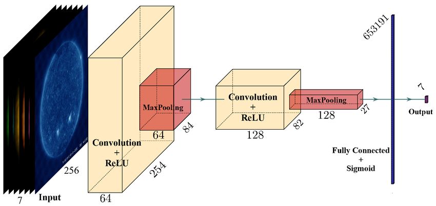
ing across the different channels will make a multi-channel CNN Fig. 3. The CNN architectures used in this paper. At the top the single-
architecture more effective than a single channel CNN that only channel architecture with a single wavelength input and composed of
exploit inter-channel structure correlations. The first model con- two blocks of a convolutional layer, ReLU activation function and max
siders a single channel as input in the form of a tensor with shape pooling layer, followed by a fully connected (FC) layer and a final sig-
1 × 256 × 256 and have a single degradation factor α as output. moid activation function. At the bottom the multi-channel architecture
The second model takes in multiple AIA channel images simul- with a multi wavelength input and composed of two blocks of a convolu-
taneously as an input with shape n × 256 × 256 and output n tional layer, ReLU activation function and max pooling layer, followed
by a fully connected (FC) layer and a final sigmoid activation function.
degradation factors α = {αi , i ∈ [1, ..., n]}, where n is the number Figures constructed with Iqbal (2018)
of channels as indicated in Fig. 3.
The single- and multi-channel architectures are described in We use the open-source software library PyTorch (Paszke
(Fig. 3). They both consist of two blocks of a convolutional layer et al. 2017) to implement the training and inference code for the
followed by ReLU (rectified linear unit) activation function (Nair CNN.
& Hinton 2010) and a max pooling layer. These are followed by
a fully connected (FC) layer and a final sigmoid activation func- 3.3. Training Process
tion that is used to output the dimming factors. The first convolu-
tion block has 64 filters, while the second convolution block has The actual degraded factors αi (t) (where t is the time since the
128. In both convolution layers the kernel size is 3, meaning the beginning of the SDO mission, and i is the channel) trace a single
filters applied on the image are 3 × 3 pixels, and the stride is 1, trajectory in an n-dimensional space starting with αi (t = 0) = 1
meaning that the kernel slides through the image 1 pixel per step. ∀ i ∈ [1, ..., n] at the beginning of the mission. During training,
No padding is applied (i.e., no additional pixels are added at the we intentionally exclude this time-dependence from the model.
border of the image to avoid a change in size). The resulting to- This is done by (1) using the SDOML dataset which has already
tal learnable parameters (LP) are 167, 809 for the single-channel been corrected for degradation effects, (2) not assuming any re-
model and 731, 143 for the multi-channel model. The final con- lation between t and α and not using t as an input feature, and (3)
figurations of the models’ architectures were obtained through a temporally shuffling the data used for training. As presented in
grid search among different hyperparameters and layer config- section 3.1, we degrade the each set of multi-channel images C
urations. More details of the architectures can be found in Ap- by a unique α = {αi , i ∈ [1, ..., n]}. We then devised a strat-
pendix B. egy such that from one training epoch to the next, the same set
Article number, page 4 of 12Luiz F. G. dos Santos et al.: Multi-Channel Auto-Calibration for the Atmospheric Imaging Assembly using Machine Learning
of multi-channel images can be dimmed by a completely inde- Table 1. The mean squared error (MSE) for all combinations proposed
pendent set of α dimming factors. This is a data augmentation in Section 3.4. The top-left cell is for the scenario when there exists a
cross-channel correlation and a relation between brightness and size of
and regularization procedure which allows the model to general- the artificial Sun. The top-right cell, has is the loss with a cross-channel
ize and perform well in recovering dimming factors over a wide correlation but not the relation between brightness and size. The bottom
range of solar conditions. left cell has the loss when there is no cross-channel correlation, but it has
The training set comprises multi-channel images C obtained a relation between brightness and size. The bottom right cell presents
during the months of January to July from 2010 to 2013 obtained the loss when the parameters are freely chosen.
every six hours, amounting to a total of 18, 970 images in 2, 710
timestamps.The model was trained using 64 samples per mini- Brightness and size
batch and the training has been performed for 1, 000 epochs. In correlation
the concept of minibatch we don’t use the full dataset to calcu- Yes No
late the gradient descent and propagate back to update the pa- Cross-channel Yes 0.017 0.023
rameters/weights of the network. We correct the weights as the correlation No 0.027 0.065
model is still going through the data. This way, we lower the
computation cost, and yet we’re still get lower variance than by
using whole dataset to calculate the gradient. As a consequence (a) and (b) influences performance. To evaluate this test we will
of our data augmentation strategy, after 1000 epochs the model use the MSE loss and expect the presence of both (a) and (b) to
has been trained with 2, 710, 000 unique sets of (input, output) minimize this loss.
pairs, since we used different set of α each epoch. We used the The test result of the multi-channel model with artificial solar
Adam optimizer (Kingma & Ba 2014) in our training with an images is shown in Table 1. We can see that when A0 ∝ σ (linear
initial learning rate of 0.001 and the mean squared error (MSE) relation between size and brightness) and Ai = Ai0 (i.e., depen-
of the the predicted degradation factor (αP ) and the ground truth dence across channels; here i superscript denotes A0 raised to the
value (αGT ) was used as the training objective (loss). i-th power), the CNN solution delivered minimal MSE loss (top-
The test dataset, i.e., the sample of data used to provide an left cell). Eliminating the inter-channel relationship (i.e., each Ai
unbiased evaluation of a model fit on the training dataset, holds was randomly chosen) or the relation between brightness Ai and
images obtained during the months of August to October be- size σ, the performance suffered increasing the MSE loss. Ul-
tween 2010 and 2013, again every six hours per day, totaling timately, when both Ai and σi were randomly sampled for all
9, 422 images over 1, 346 timestamps. The split by month be- channels, the model performed equivalently to randomly guess-
tween the training and test data has a two fold objective: (1) it ing/regressing (bottom-right cell) and having the greater loss of
prevents the bias due to the variation in the solar cycle thereby all tests. These experiments confirm our hypothesis and indi-
allowing the model to be deployed in future deep space missions cate that a multi-channel input solution will outperform a single-
forecasting α for future time steps, and (2) it ensures that the channel input model, in presence of relationships between the
same image is never present in both the datasets (any two im- morphology of solar structures and their brightness across the
ages adjacent in time will approximately be the same), leading channels.
to a more precise and a comprehensive evaluation metric.
3.5. Reconstruction of the Degradation Curve using the CNN
3.4. Toy Model Formulation to Probe the Multi-Channel Models
Relationship
In order to evaluate the model in a different dataset from the
Using the described CNN model, we tested the hypothesis us- one used in the training process, we use both single-channel
ing a toy dataset, which is simpler than the SDOML dataset. We and multi-channel CNN architectures to recover the instrumen-
tested if the physical relationship between the morphology and tal degradation over entire period of SDO (from 2010 to 2020).
brightness of solar structures (e.g., ARs, coronal holes) across To produce the degradation curve for both CNN models we use
multiple AIA channels would help the model prediction. For this an equivalent dataset of the SDOML dataset but without com-
purpose, we created artificial solar images, in which a 2D Gaus- pensating the images for degradation and having data from 2010
sian profile is used (Equation 1) to mimic the Sun as an idealized to 2020. All other pre-processing steps including masking the
bright disk with some center-to-limb variation: solar limb, re-scaling the intensity etc. remain unchanged. The
CNN’s estimates of degradation are then compared to the degra-
dation estimates obtained from cross-calibration with irradiance
Ci (x, y) = Ai exp (−[x2 + y2 ]σ−2 ), (1) measurements, computed by the AIA team using the technique
described in (Boerner et al. 2014).
where A is the amplitude centered at (0, 0), characteristic width The cross-calibration degradation curve relies on the daily
σ, and x and y, are the coordinates at the image. σ is sampled ratio of AIA observed signal to the AIA signal predicted by
from a uniform distribution between 0 and 1. These images are SDO-EVE measurements up through the end of EVE MEGS-
not meant to be a realistic representation of the Sun. However, A operations in May 2014. From May 2014 onwards, the ra-
as formulated in Eq. 1, they include two qualities we posit to be tio is computed using the FISM model (Chamberlin et al. 2020)
essential for allowing our auto-calibration approach to be effec- in place of the EVE spectra. FISM is tuned to SDO-EVE, so
tive. The first is the correlation of intensities across wavelength the degradation derived from FISM agrees with the degradation
channels (i.e., ARs tend to be bright in multiple channels). The derived from EVE through 2014. However, the uncertainty in
second is the existence of a relationship between the spatial mor- the correction derived from FISM is greater than that derived
phology of EUV structures with their brightness. This toy dataset from EVE observations, primarily due to the reduced spectral
is designed so that we can independently test how the presence resolution and fidelity of FISM compared to SDO-EVE. While
of (a) a relation between brightness Ai and size σ, and (b) a re- the EVE-to-AIA cross-calibration introduced errors of approxi-
lation between Ai for various channels; and the presence of both mately 4% (on top of the calibration uncertainty intrinsic to EVE
Article number, page 5 of 12A&A proofs: manuscript no. main
itself), the FISM-to-AIA cross-calibration has errors as large as 304 Å
25%.
We examined both V8 and V9 of the cross-calibration degra- 60 Reference Image Mode
dation curve. The major change from V8 calibration (released Dimmed Image Mode
in November 2017, with linear extrapolations extending the ob-
Reference Image Hist.
served trend after this date) to V9 (July 2020) is based on the 50 Dimmed Image Hist.
analysis of the EVE calibration sounding rocket flown on 18
June 2018. The analysis of this rocket flight resulted in an ad- 40
Number of pixels
justment in the trend of all channels during the interval covered
by the FISM model (from May 2014 onwards), as well as a 20%
shift in the 171 Å channel normalization early in the mission. 30
This changes become more clear when looking at Fig. 6 at Sec.5.
The uncertainty of the degradation correction during the period
prior to May 2014, and on the date of the most recent EVE rocket 20
flight, is dominated by the ∼ 10% uncertainty of the EVE mea-
surements themselves. For periods outside of this (particularly
periods after the most recent rocket flight), the uncertainty is a 10
combination of the rocket uncertainty and the errors in FISM in
the AIA bands (approximately 25%). 0
Moreover we obtain and briefly analyze the feature maps 0 50 100 150 200 250 300 350 400
from the second max pooling layer from the multi-channel Intensity [DN/pixel/s]
model. Feature map is simply the output of one mathematical fil-
ter applied to the input. Looking at the feature maps we expand Fig. 4. Histograms of the pixel values for 304 Å channel. In blue the
our understanding of the model operation. This process helps to histogram for the refence image and in red the histogram for the dimmed
shine light over the image processing and provides insight into image. The y-axis is the number of pixels, and the x-axis is the pixel
intensity [DN/px/s]. The modes are marked with blue and red line for
the internal representations combining and transforming infor-
the reference and dimmed images respectively.
mation from seven different EUV channels into the seven dim-
ming factors.
pixels of interest and 0 the rest. Finally, we use this mask to ex-
tract the co-spatial quiet Sun (less active) pixels from each AIA
4. Baseline Model channel and compute the respective 1D histograms of the inten-
We compare our DNN approach to a baseline motivated by the sity values as shown in Fig. 4. Now, based on the assumption that
assumption that the EUV intensity outside magnetically ARs, the intensity of the quiet Sun area does not change significantly
i.e. the quiet Sun, is invariant in time (a similar approach is also over time (as discussed in the preceding section), we chose to
considered for the in-flight calibration of some UV instruments, artificially dim these regions by multiplying them with a con-
e.g. Schühle et al. 1998). A similar assumption in measuring the stant random factor between 0 and 1. Naturally, values close to 0
instrument sensitivity of the Solar & Heliospheric Observatory will make the images progressively dimmer. The histograms for
(SOHO, Domingo et al. 1995) CDS was also adopted by Del the dimmed and the original (undimmed) quiet Sun intensities
Zanna et al. (2010), where they assumed that the irradiance vari- for the AIA 304 Å channel are shown in Fig. 4. The idea is to
ation in the EUV wavelengths is mainly due to the presence of develop a non-machine learning approach that could be used to
ARs on the solar surface and the mean irradiance of the quiet retrieve this dimming factor.
Sun is essentially constant over solar cycle. Though there are From Fig. 4 we find that both the dimmed and undimmed
evidences of small-scale variations in the intensity of quiet Sun 1D histograms have a skewed shape, with a dominant peak at
when observed in the transition region (Shakeri et al. 2015), their lower intensities and extended tails at higher intensities. Such
contribution is insignificant in comparison to their AR counter- skewed distribution for the quiet Sun intensities has been re-
parts. The baseline and its method is described in the following ported by various studies in the past (see Shakeri et al. 2015),
passage. where they have been modelled as either a sum of two Gaussians
It is important to remark that we use exactly the same data (Reeves et al. 1976) or a single log-normal distribution (Griffiths
pre-processing and splitting approach like the one used for the et al. 1999; Fontenla et al. 2007). Despite an increased number of
neural network model described in Sect. 3.3. From the processed free parameters in double Gaussian fitting, Pauluhn et al. (2000)
dataset, a set of reference images per channel, Cref , are selected showed that the observed quiet Sun intensity distribution could
at time t = tref . Since the level of solar activity continuously be fitted significantly better with a single log-normal distribu-
evolves in time, we only select the regions of the Sun that cor- tion. The skewed representation, such as the one shown for the
respond to low activity, as discussed in the preceding paragraph. 304 Å channel, was also observed for all the other EUV chan-
Furthermore, the activity level is decided based on co-aligned nels, indicating that the criterion for masking the quiet Sun pixels
(with AIA) magnetic field maps from HMI. To define these re- described here is justified.
gions, we first make a square selection with a diagonal of length We then compute the mode (most probable value) of both
2R centered at R = 0 of the solar images, so as to avoid LOS the dimmed and undimmed log-normal distributions and indi-
mp
projection effects towards the limb. We then apply an absolute cate them by Ii,ref (where i implies the AIA channel under con-
global threshold value of 5 Mx cm−2 on the co-aligned HMI sideration and mp stands for the modal value for the undimmed
mp
LOS magnetic field maps corresponding to t = tref , such that images), and Ii representing the modal intensity value for the
only those pixels that have BLOS less than the threshold are ex- corresponding images dimmed with a dimming factor (say αi ).
tracted, resulting in a binary mask with 1 corresponding to the These are indicated by blue and red vertical lines in Fig. 4. Sub-
Article number, page 6 of 12Luiz F. G. dos Santos et al.: Multi-Channel Auto-Calibration for the Atmospheric Imaging Assembly using Machine Learning
sequently, the dimming factor is obtained by computing the ratio 0.010 Training Loss
between the two most probable intensity values according to the Testing Loss
following equation:
0.008
mp
Ii
αi := mp (2)
Loss (MSE)
Ii,ref 0.006
Since both distributions are essentially similar except for the
dimming factor, we suggest that such a ratio is efficient enough
to retrieve αi reliably forming a baseline against which the neural 0.004
network models are compared. The efficiency of the baseline in
recovering the dimming factor is then evaluated according to the
success rate metric and the results for all channels are tabulated 0.002
in Table 2.
0 200 400 600 800 1000
5. Results and Discussions Epoch
5.1. Comparing the performances of the baseline model with
different CNN architectures Fig. 5. Graphic of the evolution of training and testing MSE loss through
the epochs.
The results of the learning algorithm are binarized using five dif-
ferent thresholds: the absolute value of 0.05 and relative values
of 5%, 10%, 15%, and 20%. If the absolute difference of the improvements for almost all the EUV channels. Clearly, the suc-
predicted degradation factor (αP ) and the ground truth degrada- cess rates belonging to the red category is much lesser compared
tion factor (αGT ) is smaller than the threshold, it is considered a to the former models implying that the mean success rate is the
success αP ; otherwise, it is not a success. We then evaluate the highest across all tolerance levels. The multi-channel architec-
binarized results by using the success rate, which is the ratio of ture recovers the degradation (dimming) factor for all channels
success αP and total amount of αP . We chose different success with a success rate of at least 91% for a relative tolerance level
rate thresholds to gauge model, all of which are smaller than the of 20% and a mean success rate of ∼ 94%. It is also evident
uncertainty of the AIA calibration (estimated as 28% by Boerner that this model outperforms the baseline and the single-channel
et al. 2012). model for all levels of relative tolerances. For any given level
The baseline, single-channel, and multi-channel model re- of tolerance the mean across all channels increased significantly,
sults are summarized in Table 2. The different colors are for dif- for example with absolute tolerance of 0.05 the mean increase
ferent success rates: green is for success rates greater than 90%, from 78% to 85%, even changing its color classification. In ad-
yellow for success rate between 80% and 90%, and red is for dition, the success rate is consistently the worst for 335 Å and
success rate lower than 80%. 211 Å channels across all tolerances, whereas the performance
A detailed look at Table 2 reveals that for an absolute tol- of the 131 Å channel is the best.
erance value of 0.05, the best results for the baseline are 86% Looking at specific channels we can see that 304 Å does
(304 Å) and 76% (131 Å), and a mean success rate of ∼ 51% consistently well through all the models with not much variation,
across all channels. As we increase the relative tolerance levels,
which wasn’t expected. Now observing 171 Å, it does well in the
the mean success rate increases from 27% (for 5% relative tol-
baseline and in the multi-channel model but surprisingly it has its
erance) to 66% (with 20% relative tolerance) and with a 39%
maximum performance in the single-channel model, through all
success rate in the worst performing channel (211 Å).
tolerances, and a remarkable 94% success rate with a tolerance
Investigating the performance of the CNN architecture with
of 0.05. In opposite to 171 Å, channels 211 Å and 335 Å have a
a single input channel and an absolute tolerance level of 0.05, we
poor performance in the baseline and the single-channel models,
find that this model performed significantly better than our base-
and they have a significant improvement in the multi-channel
line with much higher values of the metric, for all the channels.
model as expected and hypothesised by this paper.
The most significant improvement was shown by the 94 Å chan-
nel with an increase from 32% in the baseline model to about Observing the Fig.5, we can see the training and test MSE
70% in the single input CNN model, with an absolute tolerance loss curve evolving by epoch. Based on the results from the Ta-
of 0.05. The average success rate bumped from 51% in the base- ble 2 and comparing the training and test loss curves in Fig. 5
line to 78% in the single-channel model. The worst metric for we can see the model does not heavily overfit in the range of
epochs utilised and it presents stable generalization performance
the single-channel CNN architecture was recorded by the 211 Å on test results. We stopped the training before epoch 1000, see-
channel, with a success rate of just 63%, which is still signif- ing only marginal improvements achieved in the test set over
icantly better than its baseline counterpart (31%). Furthermore, many epochs.
with a relative tolerance value of 15%, we find that the mean suc-
cess rate is 85% for the single-channel model, which increases Overall the result shows higher success rates for the CNN
to more than 90% for a 20% tolerance level. This is a promising models, particularly for the multi-channel model, which was pre-
result considering the fact that the errors associated with the cur- dicted by the toy problem, and for higher tolerances.
rent state-of-the-art calibration techniques (sounding rockets) is
∼ 25%. 5.2. Modelling Channel Degradation over Time
Finally, we report the results from the multi-channel CNN
architecture in the last section of Table 2. As expected, the per- In this section we discuss the results obtained when comparing
formance in this case is the best of the models with significant the AIA degradation curves V8 and V9, with both single-channel
Article number, page 7 of 12A&A proofs: manuscript no. main
Table 2. Results of the baseline and CNN models applied to all the EUV AIA channels. The Table is divided in three sections: Baseline, Single-
Channel and Multi-Channel model. From left, the channel number, the success rates for the baseline, the success rates for the single-channel CNN
model, and the success rates, for the multi-channel CNN model, each model performance is considered at different tolerance levels. At the bottom,
the mean of the success rate across all the channels. Color green is for success rates greater than 90%, yellow for success rate between 80% and
90% and red is for success rate lower than 80%.
Baseline Single-Channel Model Multi-Channel Model
Channel
0.05 5% 10% 15% 20% 0.05 5% 10% 15% 20% 0.05 5% 10% 15% 20%
94 Å 32% 08% 18% 28% 40% 70% 37% 61% 78% 87% 82% 48% 73% 85% 92%
131 Å 76% 50% 73% 86% 96% 94% 72% 92% 98% 99% 99% 76% 94% 97% 99%
171 Å 58% 27% 48% 66% 85% 93% 70% 93% 97% 99% 84% 48% 72% 86% 93%
193 Å 38% 13% 27% 44% 53% 73% 41% 69% 85% 93% 90% 59% 85% 94% 98%
211 Å 31% 11% 21% 29% 39% 63% 30% 53% 71% 84% 76% 41% 68% 82% 92%
304 Å 86% 66% 89% 95% 100% 90% 65% 89% 97% 99% 94% 62% 86% 93% 96%
335 Å 38% 13% 29% 42% 51% 62% 31% 54% 69% 80% 73% 39% 65% 82% 91%
Mean 51% 27% 43% 56% 66% 78% 50% 73% 85% 92% 85% 53% 77% 89% 94%
and multi-channel CNN models. This process was performed us- Table 3. Goodness of fit metrics for single-channel and multi-channel
ing a dataset equivalent to the SDOML but with no correction for models with reference to the V9 degradation curve. The first metric is
the Two-Sample Kolmogorov-Smirnov Test (KS), and second metric is
degradation and data period from 2010 to 2020. This tests both the Fast Dynamic Time Warping.
models for real degradation suffered by AIA from 2010 to 2020.
Figure 6 presents the results of our analysis for all the seven Single-Channel Multi-Channel
AIA EUV channels. In each panel, we show four quantities: Channel
the degradation curve V9 (solid black line), the degradation KS DTW KS DTW
curve V8 (solid gray line), predicted degradation from the single- 94 Å 0.485 7.120 0.568 9.624
channel model (dashed colorful line) and multi-channel model
(solid colorful line). The shaded gray band depicts the region 131 Å 0.346 2.711 0.275 1.624
covering 25% variation (error) associated with the V9 degrada- 171 Å 0.298 3.074 0.329 3.549
tion curve and the colorful shaded areas are the standard devia- 193 Å 0.211 1.829 0.244 2.080
tion of the single- and multi-channel models. The dashed vertical 211 Å 0.305 2.850 0.242 2.807
line coincides with the day (25 May 2014), the last day of EVE 304 Å 0.282 1.412 0.100 1.311
MEGS-A instrument data. It is important to note that MEGS- 335 Å 0.212 2.539 0.141 2.839
A was earlier used for the sounding rocket calibration purposes,
the loss of which caused both the V8 and V9 degradation curves
to become noisier in the future. Szenicer et al. (2019) used deep Table 3 contains two different metrics for evaluating the
learning to facilitate a virtual replacement for MEGS-A. goodness of fit of each CNN model with the V9 degradation
Observing the different panels of Fig. 6, we can see that even curve. The first is the Two-Sample Kolmogorov–Smirnov Test
though we trained both the single and multi-channel models with (KS), which determines whether two samples come from the
the SDOML dataset that was produced and corrected using the same distribution (Massey Jr. 1951), and the null hypothesis as-
V8 degradation curve, both CNN models predict the degradation sumes that the two distributions are identical. The KS test has
curves for each channel quite accurately over time, except for the advantage that the distribution of statistic does not depend on
94 Å and 211 Å channel. However, the deviations of the pre- cumulative distribution function being tested. The second metric
dicted values for these two channels fall well within the 25% is the Fast Dynamic Time Warping (DTW, Salvador & Chan
variation of the V9 calibration curve. In fact, the CNN predic- 2007), which measures the similarity between two temporal se-
tions have even better agreement with V9 than the V8 calibra- quences that may not be of the same length. This last one is im-
tion for most of the channels. That hints at the conclusion that portant since statistical methods can be too sensitive when com-
the CNN is picking up on some actual information that is per- paring two time series. DTW has distance between the series as
haps even more responsive to degradation than FISM. The latest an output, and as a reference the DTW for the different EUV
degradation curve (V9) was updated recently in July 2020 and channels between the V8 and V9 degradation curves are: 94 Å-
the change from V8 to V9 might have easily caused an impact 72.17, 131 Å- 13.03, 171 Å-9.82, 193 Å-30.05, 211 Å-16.86,
while training the models. Moreover, the more significant devia- 304 Å-7.02 and 335 Å-5.69.
tion of 94 Å channel in the early stages of the mission is due the Similar to Fig. 6 we find in Table 3, that the predictions from
fact we limited our degradation factor to be less than one. both the single-channel and multi-channel models overlap sig-
From the predicted calibration curves computed from the nificantly both in terms of the metric and the time evolution.
single- and multi-channel models, we see that they have a sig- Except for the 94 Å channel, all others have very close metric
nificant overlap throughout the entire period of observation. The values, well within a given level of tolerance. A low value of the
single-channel model predictions however, have a more signif- KS test metric suggests that the predictions have a similar distri-
icant variation for channels 211 Å, 193 Å and 171 Å. For a bution as the observed V9 calibration curve which also indicates
systematic evaluation and a comparison among the results of the the robustness of our CNN architecture. KS test agrees well with
two models across channels, we calculated some goodness of fit DTW, where the values obtained are smaller to the reference val-
metrics and the results are shown in Table 3. ues (as indicated earlier) between the V8 and the V9 calibration
Article number, page 8 of 12Luiz F. G. dos Santos et al.: Multi-Channel Auto-Calibration for the Atmospheric Imaging Assembly using Machine Learning
Fig. 6. Channels degradation over Time. From top to bottom: Channel 94 Å (blue) and 131 Å (yellow), 171Å (green) and 193 Å (red), 211 Å (pur-
ple) and 304 Å (brown) and 335 Å (magenta). The solid black (gray) curve is the degradation profile of AIA calibration release V9 (V8). The gray
shaded area correspond to the 25% error of the degradation curve V9. The colorful shaded areas are the standard deviation of the CNN models.
The vertical black dashed line is the last available observation from EVE MEGS-A data and the vertical gray dashed line is the last training date.
Article number, page 9 of 12A&A proofs: manuscript no. main
curves. Overall, the metric analysis for the goodness of fit be- channel relationship among different EUV channels by introduc-
tween the predictions and the actual calibration curve (V9) show ing a robust novel method to correct for the EUV instrument time
that the CNN models perform remarkably well in predicting the degradation. We began with formulating the problem and setting
degradation curves despite being trained only on the first three up a toy model to test our hypothesis. We then established two
years of the observations. CNN architectures that consider multiple wavelengths as input
to auto-correct for on-orbit degradation of the AIA instrument
on board SDO. We trained the models using SDOML dataset,
5.3. Feature Maps and further augmented the training set by randomly degrading
images at each epoch. This approach made sure that the CNN
model generalizes well to data not seen during the training, and
193 Å
1 we also developed a non-ML baseline to test and to compare
its performance with the CNN models. With the best trained
CNN models, we reconstructed the AIA multi-channel degra-
dation curves of 2010-2020 and compared with the sounding-
Pixel Intensity [DN/s/pixel]
rocket based degradation curves V8 and V9.
Our results indicate that the CNN models significantly out-
perform the non-ML baseline model (85% vs. 51% in terms of
0.5 the success rate metric), for a tolerance level of 0.05. In addi-
tion, the multi-channel CNN also outperforms the single-channel
CNN with 78% success rate with absolute 0.05 threshold. This
result is consistent with the expectation that correlations between
structures in different channels, and size (morphology) of struc-
tures and brightness can be used to compensate for the degra-
dation. To further understand the correlation between different
channels, we used the concept of feature maps to shed light over
0 this aspect and see how the filters of the CNNs were being ac-
tivated. We did see that the CNNs learned representations that
0.1
Feature weights
make use of the different features within solar images but further
work needs to be done in this aspect to establish a more detailed
0.05 interpretation.
We also found that the CNN models reproduce the most
0 recent sounding-rocket based degradation curves (V8 and V9)
very closely and within their uncertainty levels. This is particu-
larly promising, given that no time information has been used in
Fig. 7. Feature maps obtained from the last layer of CNN of our model. training the models. For some specific channels, like 335 Å, the
Top row shows a sample input in AIA 193 Å channel, and the bot- model is reproducing the V8 curve instead V9, since the SDOML
tom row shows four representative feature maps out of one hundred and
twenty eight different feature maps from the final convolutional layer of
was corrected using the former. The single-channel model could
the multi-channel NN model. perform as well as the multi-channel model even though the
multi-channel presented a more robust performance when eval-
As mentioned in Sect. 3.5, the feature maps are the result of uated on the basis of their success rates.
applying the filters to an input image. That is, at each layer, the Lastly, this paper presents a unique possibility of auto-
feature map is the output of that layer. In Fig. 7 we present such calibrating deep space missions such as the one on-board the
maps obtained from the output of the last convolutional layer of STEREO spacecraft that are too far away from Earth to be cali-
our CNN. The top row shows a reference input image observed brated using sounding-rockets. The auto-calibration model could
be trained using the first months of data from the mission, assum-
at 193 Å used in this analysis, with its intensity scaled between
ing the instrument is calibrated at the beginning of the mission.
0 − 1 pixel units, and the bottom row shows 4 representative
The data volume could be an issue, and different types of data
feature maps (out of a total of 128) with their corresponding
augmentation could be used to overcome this problem, such as
weights. These maps are obtained after the final convolutional
synthetic degradation and image rotation. We also envision that
layer of the multi-channel model and it represents the result of
the technique presented here may also be adapted to imaging in-
combining all seven EUV channels as input. The predicted α
struments or spectrographs operating at other wavelengths (e.g.,
dimming factors from the model are given by the sigmoid acti-
hyperspectral Earth-oriented imagers) observed from different
vation function applied to a linear combination of these features.
space-based instruments like IRIS (De Pontieu et al. 2014).
Such mapping allows us to see that the network actually learned
to identify the different features of such full-disk solar images Acknowledgements. This project was partially conducted during the 2019 Fron-
such as the limb, the quiet Sun features, and the ARs. The reason tier Development Lab (FDL) program, a co-operative agreement between NASA
and the SETI Institute. We wish to thank IBM for providing computing power
for visualising a feature map for specific AIA images is to gain through access to the Accelerated Computing Cloud, as well as NASA, Google
an understanding of what features a model detects are ultimately Cloud and Lockheed Martin for supporting this project. L.F.G.S was supported
useful in recovering the degradation or the dimming factors. by the National Science Foundation under Grant No. AGS-1433086. M.C.M.C.
and M.J. acknowledge support from NASA’s SDO/AIA (NNG04EA00C) con-
tract to the LMSAL. S.B. acknowledges the support from the Research Coun-
cil of Norway, project number 250810, and through its Centers of Excellence
6. Concluding remarks scheme, project number 262622. This project was also partially performed with
funding from Google Cloud Platform research credits program. We thank the
This paper reports a novel ML-based approach to auto- NASA’s Living With a Star Program, which SDO is part of, with AIA, and HMI
calibration and advances our comprehension of the cross- instruments on-board. CHIANTI is a collaborative project involving George Ma-
Article number, page 10 of 12Luiz F. G. dos Santos et al.: Multi-Channel Auto-Calibration for the Atmospheric Imaging Assembly using Machine Learning
son University, the University of Michigan (USA), University of Cambridge Szenicer, A., Fouhey, D. F., Munoz-Jaramillo,
(UK) and NASA Goddard Space Flight Center (USA). A.G.B. is supported by A., et al. 2019, Science Advances, 5
EPSRC/MURI grant EP/N019474/1 and by Lawrence Berkeley National Lab. [https://advances.sciencemag.org/content/5/10/eaaw6548.full.pdf]
Software: We acknowledge for CUDA processing cuDNN (Chetlur et al. 2014), van der Walt, S., Colbert, S. C., & Varoquaux, G. 2011, Comput. in Sci. Eng.,
for data analysis and processing we used Sunpy (Mumford et al. 2020), Numpy 13, 22
(van der Walt et al. 2011), Pandas (Wes McKinney 2010), SciPy (Virtanen et al. van der Walt, S., Schönberger, J. L., Nunez-Iglesias, J., et al. 2014, arXiv e-
2020), scikit-image (van der Walt et al. 2014) and scikit-learn(Pedregosa et al. prints, arXiv:1407.6245
2011). Finally all plots were done using Matplotlib (Hunter 2007) and Astropy van Driel-Gesztelyi, L. & Green, L. M. 2015, Living Reviews in Solar Physics,
(Price-Whelan et al. 2018). 12, 1
Virtanen, P., Gommers, R., Oliphant, T. E., et al. 2020, Nature Methods, 17, 261
Wes McKinney. 2010, in Proceedings of the 9th Python in Science Conference,
ed. Stéfan van der Walt & Jarrod Millman, 56 – 61
References Wieman, S., Didkovsky, L., Woods, T., Jones, A., & Moore, C. 2016, Solar
Physics, 291, 3567
Amodei, D., Ananthanarayanan, S., Anubhai, R., et al. 2016, in International Woods, T. N., Eparvier, F. G., Hock, R., et al. 2012, Solar Physics, 275, 115
Conference on Machine Learning, 173–182 Wu, Y., Schuster, M., Chen, Z., et al. 2016, arXiv preprint arXiv:1609.08144
BenMoussa, A., Gissot, S., Schühle, U., et al. 2013, Sol. Phys., 288, 389
Bobra, M. G. & Couvidat, S. 2015, ApJ, 798, 135
Boerner, P., Edwards, C., Lemen, J., et al. 2012, Solar Physics, 275, 41
Boerner, P. F., Testa, P., Warren, H., Weber, M. A., & Schrijver, C. J. 2014,
Sol. Phys., 289, 2377
Chamberlin, R. V., Mujica, V., Izvekov, S., & Larentzos, J. P. 2020, Physica A
Statistical Mechanics and its Applications, 540, 123228
Chetlur, S., Woolley, C., Vandermersch, P., et al. 2014, arXiv e-prints,
arXiv:1410.0759
Cheung, C. M. M., Jin, M., Dos Santos, L. F. G., et al. 2019, in AGU Fall Meeting
Abstracts, Vol. 2019, NG31A–0836
Clarke, S. 2016, in EGU General Assembly Conference Abstracts, Vol. 18,
EPSC2016–18529
De Pontieu, B., Title, A. M., Lemen, J. R., et al. 2014, Sol. Phys., 289, 2733
Del Zanna, G., Andretta, V., Chamberlin, P. C., Woods, T. N., & Thompson,
W. T. 2010, A&A, 518, A49
Domingo, V., Fleck, B., & Poland, A. I. 1995, Sol. Phys., 162, 1
Fontenla, J. M., Curdt, W., Avrett, E. H., & Harder, J. 2007, A&A, 468, 695
Galvez, R., Fouhey, D. F., Jin, M., et al. 2019, The Astrophysical Journal Sup-
plement Series, 242, 7
Goodfellow, I., Bengio, Y., & Courville, A. 2016, Deep learning (MIT press)
Griffiths, N. W., Fisher, G. H., Woods, D. T., & Siegmund, O. H. W. 1999, ApJ,
512, 992
He, K., Zhang, X., Ren, S., & Sun, J. 2016, in Proceedings of the IEEE Confer-
ence on Computer Vision and Pattern Recognition, 770–778
Hunter, J. D. 2007, Computing in Science and Engineering, 9, 90
Iqbal, H. 2018, HarisIqbal88/PlotNeuralNet v1.0.0
Jiao, Z., Jiang, L., Sun, J., Huang, J., & Zhu, Y. 2019, IOP Conference Series:
Materials Science and Engineering, 611, 012071
Jungbluth, A., Gitiaux, X., Maloney, S., et al. 2019, in Second Workshop on
Machine Learning and the Physical Sciences (NeurIPS 2019), Vancouver,
Canada
Kaiser, M. L., Kucera, T. A., Davila, J. M., et al. 2008, Space Sci. Rev., 136, 5
Kim, T., Park, E., Lee, H., et al. 2019, Nature Astronomy, 3, 397
Kingma, D. P. & Ba, J. 2014, arXiv e-prints, arXiv:1412.6980
LeCun, Y. & Bengio, Y. 1995, The Handbook of Brain Theory and Neural Net-
works, 3361, 1995
Lemen, J. R., Title, A. M., Akin, D. J., et al. 2012, Solar Physics, 275, 17
Massey Jr., F. J. 1951, Journal of the American Statistical Association, 46, 68
Mumford, S. J., Freij, N., Christe, S., et al. 2020, SunPy
Nair, V. & Hinton, G. E. 2010, in Proceedings of the 27th International Con-
ference on International Conference on Machine Learning, ICML’10 (USA:
Omnipress), 807–814
Neuberg, B., Bose, S., Salvatelli, V., et al. 2019, arXiv e-prints,
arXiv:1911.04008
Oord, A. v. d., Dieleman, S., Zen, H., et al. 2016, arXiv preprint
arXiv:1609.03499
Paszke, A., Gross, S., Chintala, S., et al. 2017, in NeurIPS Autodiff Workshop
Pauluhn, A., Solanki, S. K., Rüedi, I., Landi, E., & Schühle, U. 2000, A&A, 362,
737
Pedregosa, F., Varoquaux, G., Gramfort, A., et al. 2011, J. Mach. Learn. Res.,
12, 2825
Pesnell, W., Thompson, B., & Chamberlin, P. 2012, solphys, 275, 3
Price-Whelan, A. M., Sipőcz, B. M., Günther, H. M., et al. 2018, AJ, 156, 123
Reeves, E. M., Vernazza, J. E., & Withbroe, G. L. 1976, Philosophical Transac-
tions of the Royal Society of London Series A, 281, 319
Salvador, S. & Chan, P. 2007, Intell. Data Anal., 11, 561–580
Salvatelli, V., Bose, S., Neuberg, B., et al. 2019, arXiv preprint arXiv:1911.04006
Schou, J., Scherrer, P. H., Bush, R. I., et al. 2012, Solar Physics, 275, 229
Schühle, U., Brekke, P., Curdt, W., et al. 1998, Appl. Opt., 37, 2646
Schwenn, R. 2006, Living Reviews in Solar Physics, 3, 2
Shakeri, F., Teriaca, L., & Solanki, S. K. 2015, A&A, 581, A51
Article number, page 11 of 12You can also read