Environmental Impacts of Marine SO2 Emissions - Concawe
←
→
Page content transcription
If your browser does not render page correctly, please read the page content below
report no. 1/18

Environmental Impacts
of Marine SO2
Emissions
report no. 1/18 Environmental Impacts of Marine SO2 Emissions Prepared by Concawe STF-67 members: M. E. Benavente Queiro F. Chevallier F.A. Delgado C. Diaz Garcia A. Ebbinghaus A. Jimenez Garcia J. Megeed S. Toujas E. Van Bouwel A. Zamora Concawe: L. González Bajos (Science Executive) L. Hoven (Science Executive) D. Valdenaire (Science Executive) L. White (Consultant) Reproduction permitted with due acknowledgement Concawe Brussels January 2018 I
report no. 1/18

 ABSTRACT

 This report details work that was carried out to study the impact of emissions from
 international shipping on air quality, with a focus on sulphur dioxide (SO2) emissions.
 Emission inventories are discussed and put into perspective versus emissions from
 natural sources. Air quality modelling tools have been used to assess impacts on air
 quality in EU countries as a function of distance from shore of shipping emissions.
 This work demonstrates that, compared to further land based emission reductions, it
 is generally not cost-effective to reduce emissions from shipping outside of coastal
 zones. Options to reduce fuel sulphur levels as a route to mitigate SO2 emissions from
 international shipping are compared with the use of on board techniques to remove
 SO2 from the exhaust gas stream. Finally the likely climate impact of such mitigation
 actions are assessed.

 KEYWORDS

 Marine, bunker, emissions, sulphur, SO2

 INTERNET

 This report is available as an Adobe pdf file on the Concawe website
 (www.concawe.org).

NOTE
Considerable efforts have been made to assure the accuracy and reliability of the information
contained in this publication. However, neither Concawe nor any company participating in
Concawe can accept liability for any loss, damage or injury whatsoever resulting from the use of
this information.

This report does not necessarily represent the views of any company participating in Concawe.

II
report no. 1/18

CONTENTS Page

1. INTRODUCTION 1

2. SHIPPING EMISSIONS INVENTORIES (SO2 AND CO2) 3
 2.1. EUROPE 3
 2.2. GLOBAL 5

3. REGULATORY CONTEXT 7
 3.1. INTERNATIONAL MARITIME ORGANIZATION 7
 3.2. EUROPEAN REGULATIONS 9

4. COMPLIANCE OPTIONS AND SCRUBBERS 10
 4.1. COMPLIANCE OPTIONS 10
 4.2. SCRUBBER CONSIDERATIONS 10
 4.2.1. Performance 10
 4.2.2. Energy requirements, chemicals and waste 10
 4.2.3. Environmental impact of effluent 11

5. ENVIRONMENTAL IMPACT OF SO2 EMISSIONS 13
 5.1. EUROPEAN SEA AREAS PROJECT 13
 5.1.1. European Air Quality Modelling work 13
 5.1.2. Impact as a function of distance from shore 13
 5.1.3. Global Cap versus Coastal Zone ECA 20
 5.2. EVALUATION AND COMPARISON WITH LITERATURE 22
 5.2.1. Global health impact assessments 22
 5.2.2. Contribution from natural sources 22

6. GREENHOUSE GAS AND CLIMATE IMPACTS 25
 6.1. REFINERY GHG IMPACTS 25
 6.2. AIR QUALITY AND CLIMATE COUPLING 27

7. CONCLUSIONS 29

8. GLOSSARY 30

9. REFERENCES 31

APPENDIX 1 - BACKGROUND ON SHIPPING 34

APPENDIX 2 - NATURAL AND ANTHROPOGENIC SOURCES OF SULPHUR
 EMISSIONS 36

APPENDIX 3 - AIR QUALITY MODELLING FOR POLICY MAKING 38

APPENDIX 4 - EXHAUST GAS CLEANING SYSTEMS 42

APPENDIX 5 - COASTAL ZONE MODELLING 45

 III
report no. 1/18

 SUMMARY

 This report details work that was carried out to study the impact of emissions from
 international shipping on air quality, with focus on sulphur dioxide (SO2) emissions.

 SO2 emissions are of concern because of their potential harmful effects to human
 health and the environment. Emissions from land based sources and shipping are
 regulated. In Europe, there has been a significant reduction in land based SO 2
 emissions from the 1990s, outstripping the reduction of SO 2 from shipping. As a result,
 emissions from international shipping in European waters now represent a larger
 fraction of the remaining emissions. At the global level, international shipping currently
 represents about 10% of man-made SO2 emissions. Natural sources of atmospheric
 sulphur are also significant, e.g. volcanoes. Emissions of dimethyl sulphide from
 biomass in the world’s oceans are particularly relevant. As an example, it is
 anticipated that in 2020 in the European sea areas there will be significantly more SO2
 originating from biomass than from shipping emissions.

 Regulations on fuel sulphur content from the International Maritime Organisation have
 mandated the use of low sulphur fuels in so-called Emission Control Areas (ECAs).
 Further emission reductions have been agreed and will result in a global sulphur cap
 of 0.50% starting in 2020. Apart from using low sulphur fuels, ship operators will have
 the option to use alternative fuels such as LNG or to make use of an exhaust gas
 cleaning system (scrubber) to achieve equivalent SO2 emissions while continuing to
 use higher sulphur fuels.

 The impact of SO2 emissions from maritime transport to SO2 concentrations on land
 is a strong function of the distance from shore. To illustrate this, data obtained by the
 MATCH model has been analysed to determine how the sulphate related fine
 particulate matter concentrations on land get reduced as the emission occurs further
 away from shore. On the basis of the potency of emissions thus derived, Concawe’s
 in-house Integrated Assessment Tool has been used to estimate air quality impact
 reductions on European populations by reducing SO2 emissions in coastal zones
 varying in width from 12 to 200 nautical miles. This work demonstrates that, compared
 to further land based emission reductions, it is generally not cost-effective to reduce
 emissions from shipping outside of coastal zones.

 The report also considers the greenhouse gas and climate impacts of shipping
 emission regulations. The production of fuels with lower sulphur will lead to increased
 CO2 emissions from the refining industry. Making use of on-board scrubbers will result
 in lower overall CO2 emissions versus desulphurisation of fuels in refineries.
 Furthermore there is an impact on short-lived climate forcing related to the cooling
 effect of sulphate aerosols. Due to this effect, emissions from international shipping
 have a net cooling effect on a 20+ year horizon. This cooling effect will be largely
 eliminated with the introduction of the lower global sulphur limit in 2020.

IV
report no. 1/18 1. INTRODUCTION General Background & Objectives SO2 emissions are of concern because of their potential harmful effects to human health and the environment. Since the 1990’s land based emissions of the main pollutants (SO2, NOx, NH3, VOC) contributing to one or more effects (acidification, eutrophication, ground-level ozone and secondary aerosols) have been reduced substantially (Figure 1). In particular for SO2, emission reductions from land-based sources have been very substantial. Since a number of years attention at the European and global level has also focussed on emissions from international shipping [1]. Figure 1 Twenty year emission reductions for SOx and other pollutants, from European Monitoring and Evaluation Programme (EMEP, 2013) This report aims to contribute scientific information to the debate. The specific objectives of this report are to: Provide a brief overview of marine SO2 emissions and place these into context of global and European emissions from all sources; Explore the contribution of international shipping SO2 emissions to air quality concerns on land; Provide an overview of potential routes to compliance with international regulations governing international shipping; Explore the relationship between air emissions policy and climate impacts. 1
report no. 1/18

 Technical Background
 Combustion of fuels containing sulphur leads to emissions of sulphur oxides. Most
 sulphur oxides will be in the form of SO2, but a small fraction (typically 2-4% after the
 engine) of the release may be in the form of SO 3 [2]. For this reason, sulphur oxide
 emissions are often referred to a SOx emissions, to indicate the total sulphur oxides
 emissions. SOx emissions can be estimated accurately on the basis of the sulphur
 content of the fuel and are expressed in SO2 weight equivalent.

 Once released to the atmosphere, SO2 will readily be absorbed by water droplets and
 will be oxidized to SO3, leading to the formation of sulphate, SO42- and sulphate
 aerosols. The ultimate fate of SO2 is formation of sulphate salts, which may deposit
 on land or over the oceans. The average lifetime of SO2 in the atmosphere before
 conversion is of the order of days [3]. These atmospheric transformation mechanisms
 are incorporated into the air quality models used to assess the impact of emissions.

 Air quality models are used broadly to assess impacts of emissions and explore
 potential impact of regulatory measures under consideration. This report refers to
 modelling work by various European research institutes. In addition some specific
 modelling work has been undertaken using Concawe’s in-house model, SMARTER,
 developed and maintained by Aeris Europe.

 A technical introduction to air quality modelling in the policy development context is
 provided in Appendix 3.

 Furthermore reference is made to a number of relevant scientific articles and technical
 publications.

2
report no. 1/18

2. SHIPPING EMISSIONS INVENTORIES (SO2)

2.1. EUROPE

 While European land based SO2 emissions have been reduced significantly since the
 1990’s, emissions from international shipping in European waters have been
 increasing slowly despite maximum fuel sulphur levels being limited to 4.5% in 2008
 and 3.5%S since 2012. This is illustrated by Figure 2, which shows that current SO2
 emissions from international shipping in European waters represent about 25% of the
 total SO2 emissions over the combined European Union’s land and sea areas [4].
 Emissions of SO2 from natural sources is discussed in detail in Section 5.2.2 and
 Appendix 2. In Figure 2, the contribution from volcanoes has been included to
 highlight the relative importance of natural sources, particularly in more recent years,
 where land based anthropogenic emissions have been substantially reduced.

 Figure 2 European SO2 emissions [4]

 Data on emissions for each European Sea Area can be found in a 2013 Report by
 VITO [5]. Figure 3 compares emissions in the main European sea areas. These
 figures compare well with an emission inventory for the Mediterranean developed by
 Entec for Concawe in 2007 [6]. Entec estimated the 2005 Mediterranean emissions
 at 863 kton, which is 13% higher than VITO’s estimate.

 3
report no. 1/18

 Figure 3 Shipping SO2 emissions by sea area [5]

 Figure 4 provides a more detailed overview for a 2020 base case. This base case
 takes into account the reduction in fuel S level from 3.50% to 0.50% outside of ECAs.
 This chart also distinguishes between emissions while in port or at berth (where S
 level of 0.10% is mandated) and in coastal zones versus the open seas.

 Figure 4 Shipping emissions by sea area – 2020 base scenario [5]

4
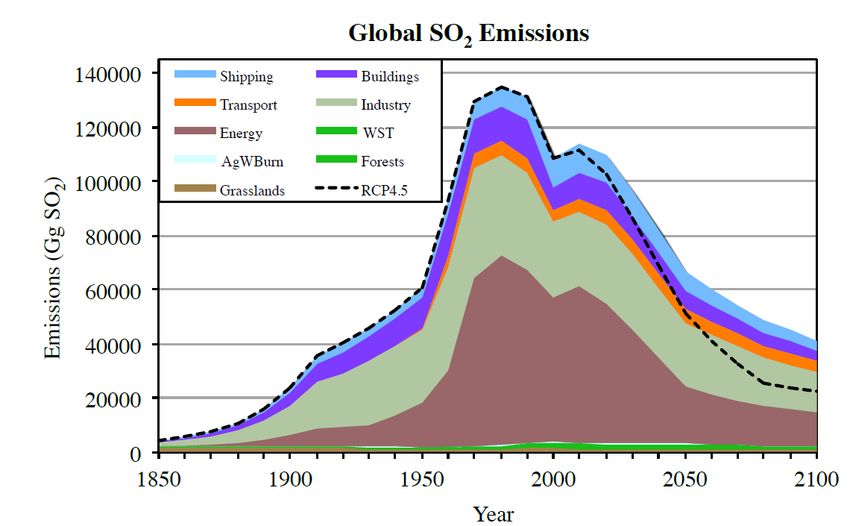
report no. 1/18

 .

2.2. GLOBAL

 The International Maritime Organisation (IMO) has commissioned several studies to
 assess the total greenhouse gas (GHG) emissions from shipping. The most recent
 update has been published in 2014 and is generally referred to as the IMO 3rd GHG
 report. Global shipping CO2 emissions were assessed to represent 2.6% of total
 global CO2 emissions [7]. The report also includes an estimate of global SO2
 emissions from international shipping, based on the estimated total fuel consumption
 and average S content of the fuels. IMO’s 3rd Greenhouse Gas Study is now widely
 used as a reference for global marine fuel demand.

 Current emission inventories are significantly lower than the projections that were
 made ahead of the 2008 financial crises. This is illustrated by the projections that were
 considered by IMO at the time of the revision of Annex VI in the 2007-2008 timeframe
 [8] as shown by the top curves in Figure 5. Table 1 illustrates that overall fuel demand
 in 2012 is lower than what had been estimated for the total fuel demand in 2007.
 Furthermore projected growth rates, as used for the 2016 assessment of fuel
 availability (see also chapter 3.1) are significantly less bullish, resulting in a projected
 fuel use in 2020 that is 30 to 37% lower than the 2007 estimates on which the revision
 of Annex VI has been based.

 In reviewing this data, we noted that the IMO 3rd Greenhouse Gas Study appears to
 underestimate the SO2 emissions reported for 2012. Based on the average fuel S
 level reported by IMO for 2012 [9] of 2.51% and 0.14% for heavy fuel oil and distillate
 fuels respectively, we estimate a total SO2 emission of 11.61 Mton/yr rather than the
 10.24 Mton/yr reported.

 Table 1 Global shipping fuel demand estimates

 Source Year Residual Distillate fuel SO2
 fuel (Mton/yr) emissions
 (Mton/yr) (Mton/yr)
 IMO Scientific 2007 286 83 16.2
 Group of Experts
 2007
 2020 382 104 22.7
 IMO 3rd GHG 2007 266 80 11.581
 report
 2012 228 64 10.2
 Concawe 2020 244 69 12.43
 extrapolation
 CE Delft (2016) 2020 269 39
 – base case
 EnSys (2016) 2020 253 88

 5
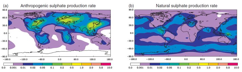
report no. 1/18

 Figure 5 Projected global SO2 emissions from international shipping

 Data sources: IMO Scientific Group of Experts Report, BLG 12/6/1, 2007
 IMO 3rd GHG report (2014), Marine and Energy Consulting Ltd, Outlook for Marine Bunker &
 Fuel Oil to 2035, May 2014

 For the extrapolations based on the current marine fuel demand estimates in Figure
 5 we have used the IMO reported sulphur levels for 2012 [9].

 The current projections in Figure 5 are still slightly higher than the data used in a
 recent scientific study that evaluated the health impacts of SOx emissions from
 international shipping[10]. They are aligned with historical ship fuel consumption and
 emissions estimates[11].
 In summary, the discussion at MEPC (Marine Environment Protection Committee) to
 agree the update of MARPOL Annex VI in 2008 was based on assumptions of high
 GDP growth, with shipping demand linked to GDP growth resulting in a significant
 growth of shipping SOx emissions. When new fuel consumption data and revised
 projections for demand growth are taken into account significantly lower SOx
 emissions, even without a 0.50%S global cap from 2020 are evident. With the
 emissions cap in place, global shipping emissions will be very significantly reduced.

 It is relevant to compare emissions from international shipping with emissions from
 other man-made sources and emissions from natural sources. SO2 emissions from
 international shipping represent about 10% of anthropogenic emissions. Amongst the
 natural sources of SO2 emissions, both volcanoes and emissions of dimethylsulphide
 (DMS) from biomass in the oceans are larger sources of atmospheric sulphur than
 international shipping. In 2014, the contribution of volcanic sources of SO2 emissions
 in the European region were officially reported at some seven times those from
 shipping sources; the contribution of DMS at some 1.3 times shipping SO2 emissions
 [12]. At the same level of DMS emissions, in 2020 this source would be some seven
 times higher than emissions from ship sources in the same sea areas. Further
 information on natural sources of atmospheric sulphur emissions is provided in
 Appendix 2.

6
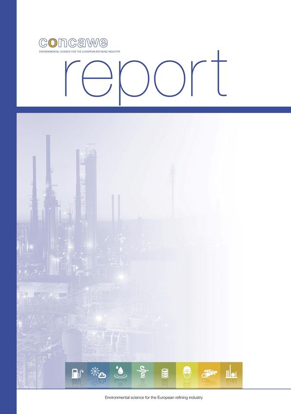
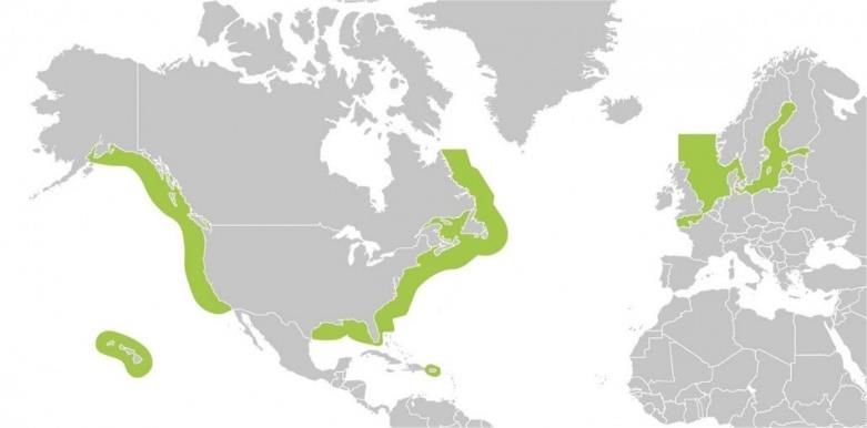
report no. 1/18

3. REGULATORY CONTEXT

3.1. INTERNATIONAL MARITIME ORGANIZATION

 International shipping is regulated at the international level by the International
 Maritime Organization (IMO). IMO is a UN organization, based in London. Air pollution
 from international shipping is regulated under the International Convention for the
 Prevention of Pollution from Ships, 1973, as modified by the Protocol of 1978 relating
 thereto and by the Protocol of 1997( MARPOL). Air emissions are covered by Annex
 VI of MARPOL which entered into force in 2005. The Annex was substantially
 modified in 2008 with the modifications taking effect in 2010.

 SOx emissions from international shipping

 One key provision of MARPOL Annex VI, Regulation 14, concerns SOx emissions.
 These are regulated by specification of a maximum sulphur level in the fuel.

 The regulation specifies different limits for operating inside and outside Emissions
 Control Areas (so called SOx ECAs) and these follow a stepped reduction over time
 as shown below:

 The Baltic Sea, the North Sea, the English Channel, and the coastline of North
 America (200NM) are currently Emission Control Areas (ECAs) where special
 emission limits apply. In the ECAs, on 1 January 2015, the maximum permitted
 sulphur content for marine fuel was reduced from the previous 1% to 0.10%.
 ECAs can also be applicable to NOx emissions. Any ECA, whether for SOx or NOx,
 should be set up in accordance with the criteria given under Appendix III of Annex VI
 which includes the requirement to demonstrate that the implementation of such an
 ECA is cost effective compared to further land based controls.
 Figure 6 shows the geographical extent of the SOx ECA areas.The rest of the world
 is subject to the “global IMO” limit. The implementation date of the reduction in the
 maximum “global IMO” sulphur content from 3.50% to 0.50% was subject to a fuel
 availability review to be completed by 2018. IMO has already considered the fuel
 availability study at the October 2016 meeting of the Marine Environment Protection
 Committee and concluded that the refining industry “has the capability to supply
 sufficient quantities of marine fuels with a sulphur content of 0.50% m/m or less”.
 Hence the implementation date for reducing the maximum fuel S level to 0.50% was
 confirmed as January 1, 2020 [13].

 7
report no. 1/18 Figure 6 Sulphur Emission Control Areas (Source: Exhaust Gas Cleaning Systems Association, www.egcsa.com) MARPOL Annex VI Regulation 4 allows flag administrations to approve alternative means of compliance that are at least as effective in terms of emission reduction as the prescribed sulphur limits in the fuels.. This means that a ship may operate on fuel with a higher sulphur content than that allowed by the regulations, provided that SOx emissions are controlled to a level which is no higher than the levels emitted if using compliant fuel. NOx emissions from international shipping MARPOL Annex VI Regulation 13 limits NOx emissions from marine diesel engines. The limits are divided into three ‘tiers’. How these tiers apply depends on the ship’s construction date and the engine’s rated speed. Tier I and Tier II limits apply to engines installed on ships built on or after 1 January, 2000, and 1 January, 2011, respectively. Tier III limits ( -80% vs. Tier I) apply to ships built on or after 1 January, 2016, if operating within the North American and US Caribbean ECA-NOx. The North Sea, Channel and Baltic Seas are scheduled to become NOx ECAs effective January 1, 2021. Particulate Matter emissions from international shipping Particulate matter (PM) emissions are not regulated as such in MARPOL Annex VI but are considered jointly with SOx emissions on the basis that lower sulphur in fuels results in lower PM emissions. These lower PM emissions are directly associated to a lower level of condensed sulphate aerosol particles in the exhaust. CO2 emissions from international shipping In 2011 the IMO added a regulatory chapter to Annex VI to include requirements on energy efficiency of ships to reduce the amount of CO 2 emissions from international 8
report no. 1/18

 shipping. These regulations introduce the concept of the Energy Efficiency Design
 Index, applicable to new ships. Baselines have been established for all common ship
 types. Newly built ships need to improve their design efficiency in three phases,
 applicable as of 2015, 2020 and 2030 respectively. For most ship types improvements
 of 10, 20 and 30% respectively are linked with each phase. In addition, all ships must
 develop a Ship Energy Efficiency Management Plan (SEEMP). These energy
 efficiency requirements can be expected to further curb growth in fuel consumption
 from international shipping. Consequently, this should also lead to lower emissions of
 SOx, PM and NOx.

 IMO continues to debate further measures to reduce GHGs from international
 shipping. As a first step IMO will implement mandatory requirements for ships of 5000
 gross tonnage and above to record and report their fuel consumption. Data collection
 will start with calendar year 2019.

 In addition to the IMO rules, local regulations may be imposed by national authorities
 in coastal waters and estuaries.

3.2. EUROPEAN REGULATIONS

 The EU Sulphur Directive (2012/33/EC) translates the IMO regulations into European
 law, while adding some specific requirements applicable in the European waters
 (territorial seas, exclusive economic zones and pollution control zones). The
 introduction of 0.50% sulphur fuels was independent of the conclusions of the global
 IMO study regarding fuel availability. In light of the October 2016 decision by IMO to
 implement the global S cap of 0.50% in 2020, this European requirement will remain
 consistent with the global requirements under Annex VI of the IMO MARPOL
 Convention.

 The European Directive however has a more stringent requirement for ships at berth
 in a European port. Within two hours of arrival, the ship has to switch to 0.1% S fuel
 until two hours before its departure at the earliest. Furthermore, passenger ships on
 a regular schedule outside of the ECAs may use fuel with a maximum S content of
 1.5% until 2020, when the lower limit of 0.50% sulphur will apply to all ships.

 9
report no. 1/18 4. COMPLIANCE OPTIONS AND SCRUBBERS 4.1. COMPLIANCE OPTIONS Regulation 14 of Annex VI of IMO’s MARPOL Convention specifies a maximum sulphur level in the fuel. Petroleum based fuels are by far the largest fraction of marine fuels currently in use. However, Regulation 18.3 of Annex VI also allows use of fuels derived by methods other than petroleum refining. In recent years LNG has received a lot of attention as an alternative fuel for marine use and there are a number of vessels either operating exclusively on LNG or having the flexibility to use either LNG or a traditional fuel. Methanol is also considered as a low S alternative fuel and biofuels are named as another option. The most popular alternative so far is enabled by Regulation 4 of Annex VI, which allows equivalent methods to achieve the environmental objectives of Annex VI, provided such methods are approved by the Ship’s Administration. Several companies are offering Exhaust Gas Cleaning Systems (EGCS), also called scrubbers, which remove SO2 from the exhaust to a level that is at least equivalent to the SO2 emission that would be achieved when low sulphur fuels are used. More details on scrubbers and their performance compared to low sulphur fuels are provided in Appendix 4. 4.2. SCRUBBER CONSIDERATIONS 4.2.1. Performance Each supplier of scrubber will provide guarantees on the levels of pollutants that their exhaust gas cleaning system can remove from a ship exhaust stream but typical figures for SOx removal are 98% [14]. Wet scrubbers may also contribute to remove a significant part of Particulate Matter and a few % of NOx. 4.2.2. Energy requirements, chemicals and waste The use of a scrubber increases the ship’s fuel consumption due to the additional energy required for the operation of the on-board scrubbing equipment: typically by around 0.3% for a freshwater scrubber (not taking into account the energy needed for the production of chemicals) and up to 2-3% for a seawater scrubber [15]. When the life cycle energy consumption of the different fuels and chemicals is taken into account, removing SO2 from exhaust gas has been shown to be less energy consuming than the alternative of removing the sulphur from fuels in refineries [15]. Fuels desulphurization requires energy: need of hydrogen, high temperatures and pressures 1 and Concawe has estimated that significant CO2 emission savings can be achieved by scrubbing. A 100% scrubber case scenario would avoid a 17 Mt/y 1 Sulphur is removed from fuels using the hydrodesulphurization process.. It requires the application of hydrogen, to break up the molecules containing sulphur and transform this sulphur to hydrogen disulphide. This in its turn can then be absorbed from the process gas, and ultimately is converted into elemental sulphur that can be stored and transported as a heated liquid or solid. These processes are energy intensive: they happen at elevated temperatures and pressures and the hydrogen required has to be produced on the basis of natural gas, whereby the carbon from the natural gas is emitted to the atmosphere as CO2 10
report no. 1/18

 increase in EU refinery CO2 emissions partially offset by 8 Mt/y increase CO2
 emissions from scrubber energy need resulting in a net saving of 9 Mt/y [16] as shown
 in Figure 7.

 Figure 7 Effect of on-board scrubbers on EU refinery CO2 emissions

 Effluent treatment of most scrubbers will generate some sludge, which needs to be
 collected and disposed of. The amount of sludge generated by scrubbers is
 approximately of 0.1 to 0.4 kg/MWh, depending on the amount of water mixed [15].
 This represents less than 10% of the ‘normal’ sludge production, which stems from
 purification of the fuel by centrifugation. Tests and analyses carried out on freshwater
 scrubbers indicate that the properties and treatment of the sludge from scrubbers are
 very similar to other engine room sludge but with lower calorific value due to higher
 water contents.

4.2.3. Environmental impact of effluent

 While at first sight, a scrubber may be seen as a device that moves pollution from air
 to water, the discharge of sulphate into the ocean does not result in an environmental
 concern. The ultimate fate of atmospheric SO2 emissions, whether manmade or from
 natural sources, is conversion to sulphate salt and oceans are a large sink of naturally
 occurring sulphate salts.

 IMO has published guidelines for the certification of scrubber systems, covering
 amongst others the allowable sulphur content in emissions, and limits on relevant
 components that may be present in the waste water discharge [17]. While the
 document is described as a “guideline,” it is given mandatory effect under MARPOL
 Annex VI, Regulation 4 and the EU Sulphur Directive (2012/33/EC).

 The guidelines specify requirements for the testing, survey and certification of an
 EGCS. The guidelines also establish limits for pH, PAHs, turbidity, nitrites and nitrates
 in wash water discharge.

 Several reports [15] [18] [19] have considered the environmental impact of scrubbers
 in marine environments. All the reports concluded, or referred to literature stating, that
 the toxicants discharged with the wash water will not lead to an exceedance of the

 11
report no. 1/18

 water environmental quality criteria in open seas or coastal areas and that the change
 in pH or alkalinity is expected to be low in the short run. On the long-term impact the
 assessments differ. While the Danish EPA (2012) emphasizes that the impact of wash
 water from scrubbers is negligible, UBA (2015) and CE Delft (2015) conclude that
 more research in these fields is necessary to be in line with the precautionary
 principles considering the cumulative effects for pH, alkalinity and non-degradable
 toxicants particularly in specific geographic areas such as ports (due to prolonged and
 concentrated pressures, limited mixing and cumulative loads from other sources) and
 ecological sensitive or vulnerable areas (e.g. Natura 2000 and/or coastal
 ecosystems).

 Nevertheless, the Danish EPA report has made a very thorough analysis, comparing
 maximum concentrations that may occur as a result of extensive use of scrubbers to
 the European and Danish water quality standards. The study considered a worst case
 scenario and demonstrated that ambient concentrations should remain below
 European and Danish environmental quality standards. Hence the study did not
 identify any concerns with the broad use of scrubbers.

 More details on the impact on seawater pH of open loop scrubber effluent can be
 found in Appendix 4.

12
report no. 1/18

5. ENVIRONMENTAL IMPACT OF SO2 EMISSIONS

5.1. EUROPEAN SEA AREAS PROJECT

5.1.1. European Air Quality Modelling work

 As part of the European Air Policy review process in 2013, the European Commission
 commissioned integrated air quality studies that evaluated different scenarios for
 further emission reductions. These scenarios included options for emission
 reductions from shipping in European waters through the establishment of further SOx
 Emission Control Areas (SECAs). This work concluded that establishment of further
 SECAs in European waters would not be a cost-effective means to achieve the
 European air quality objectives [20].

 Concawe modelling work,described in section 5.1.2 leads to conclusions that are
 consistent with this European study.

5.1.2. Impact as a function of distance from shore

5.1.2.1. Background
 The EMEP model is a chemical transport model for regional atmospheric dispersion
 and deposition of acidifying and eutrophying compounds (sulphur and nitrogen),
 ground level ozone and particulate matter covering Europe. It is a key tool within
 European air pollution policy assessments. Further information on air quality
 modelling for policy making is provided in Appendix 3. To date the EMEP model has
 been used to generate an understanding of the contribution of emissions from a given
 country or sea area to the pollutant concentrations or deposition in each receptor grid
 in the EMEP region. Through a large number of simulations, this provides country-to-
 grid or sea area-to-grid ‘source receptor’ relations. This approach however gives no
 information on the contribution from a sub area within a country or sea area.

 In the case of sea areas, in order to provide additional information on near shore
 contributions, a single scenario representing emissions from ships within 12 NM of
 EU shores was modelled. This was in addition to the sea area scenarios for each
 European sea i.e. ‘the 200 NM zone’ (from 12 NM to 200 NM) and ‘the beyond 200
 NM zone’. The resulting source receptor functions however do not provide for an
 assessment of the relationship between ‘ship distance from shore’ and the ‘impacts
 on each land grid. Such an understanding is crucial for the design of cost-effective
 ECAs as required by Annex VI of MARPOL.

5.1.2.2. Building an understanding of Impacts versus Distance from Shore
 In order to overcome this limitation, this present study used data from a small study
 by the Swedish Meteorological and Hydrological Institute (SMHI); carried out in the
 margin the Euro-Delta Project [21]. That work was undertaken using the Euro Delta
 II version of the MATCH model. A hypothetical ten kilo tonne change in SO2
 emissions from a ship travelling west from Lisbon was modelled in the MATCH CTM
 model at various distances from shore. The resulting changes in secondary PM 2.5
 concentrations in every terrestrial grid were calculated. For this work the modelling
 domain of the MATCH model was modified to include a larger part of the Atlantic, near
 Portugal.

 The baseline emissions in the Lisbon study were the emissions from the ‘Base Case
 2020 Mediterranean Sea emission scenario’ in Euro-Delta II, (scenario 54). For each

 13
report no. 1/18

 additional “distance from shore scenario”, calculations were performed with additional
 SOx (10kT/y; 95% SO2 + 5% sulphate) and primary PM2.5 (1kT/y) emissions on top of
 the baseline at five different grid points. The “extra emission” grid points were located
 at the coordinates shown in Table 2. For detailed technical information about the
 MATCH model (and the Euro-Delta II project) see the report from Euro-Delta [21]

 Table 2 Coordinates of Grid squares used in this study

 Latitude Longitude Distance to Distance to
 shore-grid point Lisbon (km)
 E (km)
 A 38.42599 -15.2314 497 525
 B 38.52946 -13.3331 331 360
 C 38.58704 -11.4293 166 194
 D 38.60000, -9.98022 40 69
 E 38.59856 -9.52358 0 32

 The corresponding grid squares are shown in Figure 8.

14
report no. 1/18

Trajectory A (SOx/PPM Scenarios, Lisbon)

 Figure 8 Grid locations

 A B C DE

 The results were used to generate an emissions potency, P z, relationship
 representing the decreasing contribution of SO 2 emissions to on-shore
 concentrations with increasing distance from shore. The points of this emissions
 potency relationship reflect the change at Lisbon in PM 2.5 concentration per kiloton of
 SO2 emissions at each of the grid points above. This trajectory was chosen because
 the prevailing on shore winds would make this a “worst case” (i.e. conservative)
 analysis. The resulting emissions potency relationship is shown in Figure 9 below.
 A full modelling exercise run for the entire European coastline with gridded emissions
 would be a worthwhile and informative future exercise.

 15
report no. 1/18

 Figure 9 Sulphate
 Sulphate PM2.5 PM2.5 Concentrations
 Concentration (µg/m3 per kt SOat Lisbon Centre (F) Versus
 2) at Lisbon Centre (F)
 Versus Distance from Shore & Designation of ZonesofWithin
 Distance from Shore & Designation Zones200nm
 within 200 NM
 1.0
 Note: SIA=Solid Inorganic Aerosol
 0.9

 0.8
 Concentration (SIA_PM2.5µg/m3 )

 0.7

 SIA_PM2.5µg/m3
 0.6
 200NM
 100
 0.5
 50
 25NM
 0.4
 12NM
 Zone Average
 0.3
 200 nm Average:

 0.2

 0.1

 0.0
 0 50 100 150 200
 Nautical miles from F

 In combination with zoned emissions data, the potency relationship described above
 was used to create weighted emissions values for use in Concawe’s in-house IAM
 tool; SMARTER. This was done by first calculating the % of total emissions
 attributable to each zone:

 % = ⁄∑5 =1 Equation 1

 In order to maintain calibration with the total sea area emissions and concentration
 potency, these zoned emissions shares, % Ei, were given a relative emissions
 potency weighting, RPz, such that:

 ∑ =1 ∗ % = 1 Equation 2

 The relative emissions potency, RPz for each band was calculated from:

 = ∗ Equation 3

 Where the adjustment coefficient was:

 . = ∑5 =1 ⁄∑5 =1( ∗ )Equation 4

 Having established the zonal concentration response potencies, the next step of the
 analysis was to determine the zonal impact response potencies. This used the
 emissions detailed in Table 32 in each zone, weighted by the ratio of potency in the
 zone divided by the average potency of the whole sea area.

2The emissions dataset was supplied by EMEP and corresponded to the 2020 base case
emissions used in their source – receptor generating runs

16
report no. 1/18

 Table 3 Banded SO2 Emissions

 sea Zone_id Buffer (NM) Emissions % of total
 SO2 (kt)
 Celtic Sea and Bay of Biscay 5 200 25 33%
 Celtic Sea and Bay of Biscay 4 100 30 39%
 Celtic Sea and Bay of Biscay 3 50 15 19%
 Celtic Sea and Bay of Biscay 2 25 6 7%
 Celtic Sea and Bay of Biscay 1 12 1 2%
 Total 77 100%

 Mediterranean Sea 5 200 33 32%
 Mediterranean Sea 4 100 23 23%
 Mediterranean Sea 3 50 21 21%
 Mediterranean Sea 2 25 10 10%
 Mediterranean Sea 1 12 14 13%
 Total 101 100%

 The zonal impact response potencies allowed the statistical Years of Life Lost (YOLL)
 impacts attributable to emissions reductions to be determined in each of the following
 zones: 0-12 NM, 12 – 25 NM, 25 – 50 NM, 50 – 100 NM and 100- 200 NM. As the
 EMEP S-R functions only provide for a single 12 to 200 NM zone, this was done by
 calculating an equivalent single zone emissions value from the weighed emissions
 potency relationship when each of the hypothetical zones was subjected to an
 emissions reduction of 50%. This single equivalent emissions value was then used
 in SMARTER to generate a delta YOLL value for the zone as a percentage of the
 delta YOLL value for a reduction of 50% for the emissions in the zone as a whole. In
 this way the impact contribution of each zone is revealed. The results are presented
 below.

5.1.2.3. Results
 Using the banded emissions data of Table 3, Figure 10 and Figure 11 show the
 percentage splits of total sea area emissions and land based impacts for the
 Mediterranean Sea and the combined Celtic Sea and Bay of Biscay areas:

 17
report no. 1/18

 Figure 10 Emissions and Impact Contribution by Zone within 200NM of EU
 Land: Mediterranean Sea

 MEDITERRANEAN SEA
 Emissions SO2 EU Population Impact (YOLL) MATCH Potency (Concentration as % First Zone)
 100%

 90%

 80%

 70%
 % share of 200 nm Zone

 60%

 50%

 40%

 30%

 20%

 10%

 0%
report no. 1/18

of near shore emissions in the Celtic Sea and Bay of Biscay compared to the
Mediterranean can be seen on the gridded emission map in Figure 12 below where
the shortest path across the Bay of Biscay is obviously taken.

In the Mediterranean, emissions beyond 50 NM are responsible for only 11% of the
impacts and in the Celtic Sea and Bay of Biscay, emissions beyond 50 NM are
responsible for 34% of the impacts, but it should be noted that overall SO2 impacts in
this region are low.

Figure 12 Gridded Ship Emissions shaded by proximity to shore; lightest
 colour within one EMEP grid (~28km) to shore

These findings have significant implications for the justification of further SECAs in
Europe. As outlined in Appendix III of MARPOL Annex VI, any application must
include a detailed assessment of the cost-effectiveness versus distance from shore.
Furthermore, given the steep near shore gradient of emissions versus impact, it is
recommended that this be done in appropriately small increments of distance,
particularly in the first 50nm from shore. Finally, any application should be based on
a move from 0.50% sulphur to 0.10% sulphur to ensure the move to a global sulphur
cap in 2020 is accounted for in the cost-effectiveness analysis compared to further
land based controls.

 19
report no. 1/18

5.1.3. Global Cap versus Coastal Zone ECA

 Given the significant and rapid attenuation of impacts as a ship sails away from the
 shore, with a focus on the Mediterranean Sea we explored the question: “at what
 distance from shore would a coastal SECA at 0.10% sulphur and a 3.50%S global
 cap give the same impacts reduction as the global sulphur cap of 0.50%?”

 To answer the above question two cases were analysed:

 i) The distance from shore at which the impacts of a 0.1% sulphur coastal zone within
 a 2.94% sulphur EEZ would be equal to the impacts of a 0.5% sulphur fuel throughout
 the 200 NM EEZ.

 ii) The distance from shore at which the impacts of a 0.1% sulphur coastal zone within
 a 2.94% sulphur Mediterranean Sea would be equal to the impacts of a 0.5% sulphur
 fuel throughout the Mediterranean Sea

 Three levels of sulphur in fuel used in the Mediterranean were modelled for their
 emission impacts on shore: 2.94% (representative actual [5]), 0.5% and 0.1%. The
 banded emissions and the derived impact potency on the EU population used were
 as those described in section 5.1.2.2 (Figure 9). Details of the methodology that has
 been used are provided in Appendix 5.

 The results are shown in Figure 13 for case i) and Figure 14 for case ii).

20
report no. 1/18

Results

Figure 13 Case i

Figure 14 Case ii

 21
report no. 1/18 Findings This analysis shows that: A coastal zone SOx ECA out to less than 45 NM would provide the same reduction in impacts on the EU population from exposure to fine particulates as would the application of the Global Sulphur Cap to the whole 200 NM zone; A coastal zone SOx ECA out to some 70 NM would provide the same reduction in impacts on the EU population as the whole Mediterranean Sea complying with the global sulphur cap. 5.2. EVALUATION AND COMPARISON WITH LITERATURE 5.2.1. Global health impact assessments A 2007 article in Environmental Science and Technology [22] drew headlines as it asserted that shipping emissions were responsible for 60000 deaths around the world. These assertions were based on extrapolation of epidemiological data that is widely used in assessing health impacts from air pollution. There are however a number of issues with this approach that have been elaborated in an IPIECA paper submitted to IMO [23]. First, it needs to be clearly recognised that such studies concern attributions to a number of different sources of pollutants, in other words, there is no direct causal relationship between a specific emission and mortality. Secondly, the study did not consider any threshold of effect. As a result, this study attributed mortality within large inland populations on the basis of extremely low contributions from international shipping to inland air quality, typically less than 0.1 µg/m3 out of total urban concentrations that may average 20 µg/m3 or more. More detailed analysis of impact data confirms that reducing shipping emissions will only have measurable impact when they occur relatively close to receptors. An illustration of this can be found in the VITO/GAINS analysis of 2013 [5] [19], which showed that additional ECAs in European waters would not be cost effective versus further land based measures that are available, with the possible exception of emissions within territorial waters (< 12 NM). An updated global impact study has been completed in 2016 to support the IMO decision making process [10]. This study concluded that reduced shipping emissions as a result of the 0.50% sulphur implementation would lead to significant reductions in ambient sulphate concentrations in coastal communities while Impacts on inland communities would be less pronounced. 5.2.2. Contribution from natural sources A recent paper by M. Yang et al [24] provides some interesting insights into the relative contributions of SO2 emissions from shipping and from natural sources. The authors set out to assess the impact of the reduction of the maximum sulphur level from 1.00% to 0.10% in the North Sea and Channel Emission Control Area (ECA) as of January 2015. They analysed continuous monitoring data from the Penlee Point Atmospheric Observatory near Plymouth. By observing diurnal variations, they were able to distinguish between SO2 originating from man-made sources and SO2 22
report no. 1/18

generated through the oxidation of dimethylsulfide (DMS) emanating from marine
biota.

Their work confirmed a significant reduction in SO2 emissions from shipping in the
Channel, in line with expectations. They observed that now half of the SO2 above the
Channel should be attributed to DMS. Evaluation of the diurnal cycle with south-
westerly winds indicates that when winds are blowing from the Atlantic Ocean, photo-
oxidation of DMS is the primary source of SO2.

A further and important source of data on the contribution of natural sources of SO 2
emissions is provided by the work undertaken under the UN Convention on Long
Range Transport of Air Pollution (CLTAP) under their European Monitoring and
Evaluation Programme (EMEP). Each year, under this programme, regional
emissions both from anthropogenic and natural sources are reported for the whole
European region. These data are used in their long range transport of air pollution
modelling work. In their most recent Status Report (1/2016) they provide detailed data
on both emissions (including DMS and emissions from volcanic activity in the region)
and on the modelled impact of these emissions on European land areas in 2014.

Figure 15 is derived from the SO2 emissions data provided in this report. For SO 2
emissions from ships in all the European Sea areas, the 2014 data is as reported.
However to provide a perspective on the impact of the 0.10% sulphur limit in SECAs
from 2015 and the mandatory global sulphur cap of 0.50% in 2020, the emissions
from shipswere adjusted based on the sulphur levels in each of the European Seas
in 2014 and the 2015 and 2020 regulatory limits. The SO2 emissions in 2014 from
natural sources and from EU land based emissions are also shown. What this figure
highlights is that in 2014 ship emissions in European seas are of the same order as
DMS emissions from those same sea areas. However, by 2020, ship emissions
(following the application of the global sulphur cap) are small compared to DMS
emissions which are some seven times higher. It is also worth noting that in 2014
volcanic activity in the region dwarfed all other contributions.

Of course we also need to consider what impact these emissions have on populations
and land ecosystems. In the same EMEP status report, data on the contribution of
these sources to individual countries are provided. Figure 16 is based on these data
using the contribution of these SO2 emissions to deposition of sulphur in a given
country as a surrogate for their impact. Here the 2020 situation is represented (i.e.
post the application of the global sulphur cap) assuming DMS emissions remain at
2014 levels – a robust assumption based on previous EMEP reports. The stacked bar
charts show the contribution to deposition of sulphur in a number of selected EU
Member States from ship activity in European Seas (Atlantic (ATL), Baltic (BAS),
Black Sea (BLS), Mediterranean (MED) and North Sea (NOS). In addition the
contribution from DMS emissions from all these sea areas is also shown. The single
points (right Y-scale) show the percentage contribution of DMS (expressed as a
percent of DMS+Ship emissions). What is very clear from this figure, consistent with
Figure 15, is that after the entry into force of the global sulphur cap, DMS emissions
dominate.

 23
report no. 1/18

 Figure 15 European Marine SO2 Emissions in the Perspective of Total
 European Emissions (Based on data from EMEP Status Report 2016)

 2014 2015-2019 From 2020

 14000

 12000
 Annual SO2 Emissions (kt)

 10000

 8000

 6000

 4000

 2000

 0
 Ships Total Marine DMS Volcanoes EU-28 Land

 Figure 16 Deposition of Sulphur from Ships and DMS on a Selection of EU
 Countries for 2020 (Based on data from EMEP Status Report 2016)

 DMS ATL BAS BLS MED NOS %DMS

 10 100%

 9 90%

 8 80%
 Deposition (units ktS)

 7 70%
 Percent DMS

 6 60%

 5 50%

 4 40%

 3 30%

 2 20%

 1 10%

 0 0%
 ly

 ay

 K
 e

 l
 k

 n
 um

 e

 ds
 d

 nd

 en
 a
 nc
 ar

 ec

 ai
 an

 U
 Ita

 ug
 w
 n

 ed
 la

 Sp
 gi

 m

 re
 a

 la
 nl

 or

 rt
 Ire
 Fr

 Sw
 el

 en

 r
 G
 Fi

 Po
 N
 he
 B

 D

 et
 N

24
report no. 1/18

6. GREENHOUSE GAS AND CLIMATE IMPACTS

6.1. REFINERY GHG IMPACTS

 . Crude oils have different compositions, but none of them match the market demand.
 Typically crudes are heavier and contain an excess of heavy fuel oil but not enough
 distillates compared to market demand (see Figure 17).

 Figure 17 Typical crude oil compositions versus European oil product
 demand
 100

 80

 60 LPG
 Naphtha/gasoline
 Kero/jet
 Gasoil/Diesel
 40 Heavy fuel oil

 20

 0
 Brent Iran light Nigerian Russian Kuwait Demand

 Refineries use available crudes to produce all the desired products at the same time,
 while allowing for crude quality variations.. More complex reefineries have invested in
 conversion units (distillate hydrocracking and residue conversion) to transform the
 lower demand heavy fuel oil into lighter, higher value products (light and middle
 distillates).

 The density and sulphur content in the crude depends on the origin, and affects the
 market value of the crude. Once the crude is split into boiling range fractions in the
 crude distillation unit (CDU), the sulphur is distributed in all the CDU output fractions,
 but is more concentrated in the heavier, high-boiling point fractions. Figure 18
 illustrates, for example, the output of a distillation unit processing a typical Brent crude
 with a sulphur content of 0.43% m/m. This crude produces a straight run heavy fuel
 oil with 0.90% m/m sulphur content.

 25
report no. 1/18

 Figure 18 Sulphur distribution of petroleum products

 Sulfur Distribution - Petroleum Products
 100%

 90%

 80% 300 ppm S

 70%

 60% LPG
 0.04 % S
 Gasoline
 50% 0.43 % S
 Kero
 0.25 % S
 40% Gasoil
 Atm. Residue
 30%
 Crude Oil
 20% 0.90 % S

 10%

 0%
 Crude Product distribution Sulfur distribution
 (by weight) (by weight)

 Considering the existing sulphur limits imposed in all refined products, refineries have
 to remove sulphur from output streams by the use of hydrodesulphurisation units.
 These units remove sulphur by reacting the sulphur-containing compounds with
 hydrogen to form hydrogen sulfide (H2S). Subsequently the elemental sulphur is
 removed in a recovery unit and sold as a product.

 Conversion and hydrodesulphurisation units consume large amounts of hydrogen).
 For this reason refineries must ensure that there is enough hydrogen production and
 sulphur recovery unit capacity to satisfy the increasing demand for lighter and lower
 sulphur products.

 Conversion and hydrodesulphurisation units are also high-energy consuming
 processes. Therefore, higher demand of distillates and more stringent sulphur limits
 result in more energy consumption in the refinery industryAny increase in energy
 consumption leads to more GHG emissions, which have an important climate impact.

 Focusing on Europe, Concawe estimated that European refineries will need 1.0 Mt/y
 of additional hydrogen production capacity and will increase their GHG emissions by
 7 Mt/y to meet the demand imposed by the marine fuel 0.50% sulphur cap in 2020
 [16]. The estimated residual marine fuel demand in Europe in 2020 amounts to 28
 million tonnes, around 5% of the total European petroleum products demand.

 Considering that the total global residual marine fuel demand in 2020 is estimated to
 be about 10 times the demand in Europe, the introduction of a global 0.50% sulphur
 limit in marine fuels can be expected to have an important climate impact due to the
 increase in GHG emissions from the global refining industry. This has indeed been
 confirmed in the 2016 EnSys/Navigistics study [25] which estimated an increase of
 21 to 44 Mton/yr to the global refining industry CO2 emissions which represents a 2.1
 to 4.4% increase.

26
report no. 1/18

6.2. AIR QUALITY AND CLIMATE COUPLING

 Net man-made impacts on the Earth’s climate are the result of complex processes.
 The largest impact on the climate due to human activity is the warming effect due to
 increasing atmospheric CO2 concentrations. However many other atmospheric
 pollutants also affect the climate. Some have a warming affect, e.g. methane and
 black carbon, while others have a cooling effect. These pollutants are called Short
 Lived Climate Forcers (SLCFs) and dealing with them is considered to be important
 to address global warming concerns, in particular as some of these compounds have
 a significantly more potent warming effect than CO2. The climate impact of these
 compounds is expressed as a Global Warming Potential (GWP) relative to the
 warming potential of CO2. As the lifetime of these compounds is substantially shorter
 than the lifetime of CO2, a compound’s GWP depends on the time frame considered.
 20 and 100 year timeframes are most commonly used to evaluate GWPs.

 SO2 emissions give rise to the formation of sulphate aerosols. These aerosols have
 a strong cooling effect. This effect is further reinforced through Aerosol Cloud
 Interactions (ACI). When considering a 20 year time frame, this overall cooling effect
 is significantly larger than the warming effect of CO2 and other pollutants, resulting in
 a net cooling effect. Over a 100 year time frame, the warming effect of CO2 becomes
 dominant, and shipping emissions will have a net warming effect. This is illustrated in
 Figure 19, based on data from the 5th Assessment Report of the International Panel
 on Climate Change [26]. Another indication of the significance of the sulphate
 aerosols effect can be found in the 2016 EMEP Status Report [12], which states:
 “Reduced European sulphur emissions unleashes the Arctic greenhouse warming:
 Using the advanced climate model NorESM1-M, the reduction of sulphate in Europe
 (EMEP region) between 1980 and 2005 is found to explain as much as about half of
 the warming observed in the Arctic during the same period. In other words, as a result
 of regulations on emissions in Europe to improve air quality and acidification of water
 and soils, a substantial portion of the dampening effect of aerosol particles has been
 removed, and consequently more of the actual warming of the Arctic due to increased
 greenhouse gas levels has emerged.”

 Figure 19 Shipping climate impact – 20 and 100 yr time horizon climate
 1 year pulse emissions

 27
report no. 1/18

 Similar observations have been made in a paper by Haakon Lindstad et al. [27]. The
 authors estimated the average global warming impact over a 20- and 100-year period
 for different scenarios. In their conclusions, the authors suggest that from an overall
 climate and environmental perspective it would be better to allow continued use of
 high sulphur fuels in open waters and to focus emission reduction efforts on coastal
 waters only.

28
report no. 1/18

7. CONCLUSIONS

 It is clear that emissions from international shipping are a significant source of
 anthropogenic SO2. However SO2 emissions from international shipping are not the
 largest source of SO2 that is generated above the oceans. The largest source of S
 emissions above the oceans is biomass, producing emissions of dimethyl sulphide
 that will oxidise to SO2 when exposed to sunlight.

 The impact of shipping emissions on health and environment on land is a strong
 function of distance from shore. Efforts to reduce emissions from international
 shipping should therefore be focused on ships operating in harbours and relatively
 close to shore. The introduction of the global S cap can be expected to significantly
 reduce contributions from shipping to ambient SO2 and sulphate aerosol
 concentrations in coastal zones that are not already covered by a SOx Emission
 Control Area. The need and justification for the establishment of further SOx Emission
 Control Areas can be evaluated on a case by case basis using the IMO guidelines for
 the establishment of ECAs.

 Removing sulphur from fuels will result in increased CO2 emissions from refineries
 related to the additional processing, including hydrogen treatment. Removing SO2
 from a ship’s exhaust by use of a scrubber offers an alternative with a lower overall
 GHG impact.

 SO2 emissions lead to the formation of sulphate aerosols that contribute to a
 substantial short-term (20 years) cooling effect. Reducing marine fuel S content as
 required under MARPOL’s Annex VI Regulations will essentially eliminate this short-
 term cooling effect.

 29
report no. 1/18

8. GLOSSARY

 CAFE Clean Air For Europe program

 CLRTAP Convention on Long-range Transboundary Air Pollution

 ECA Emission Control Area

 EEA European Economic Area

 EGCS Exhaust Gas Cleaning Systems

 EMEP European Monitoring and Evaluation Programme

 EPA Environmental Protection Agency

 GHG Greenhouse Gas

 GWP Global Warming Potential

 IMO International Maritime Organization

 LCV Lower Calorific Value (same as LHV)

 LHV Lower Heating Value (same as LCV)

 LNG Liquefied natural Gas

 MARPOL International Convention for the Prevention of Pollution from Ships

 MEPC Marine Environment Protection Committee

 MJ Megajoule

 Mton Million metric ton

 NM Nautical mile (1.852 km)

 PPE Personal Protective Equipment

 SECA Sulphur Emission Control Area

 SLCF Short Lived Climate Forcers

 TSAP Thematic Strategy on Air Pollution

 YOLL Years Of Life Lost

30
report no. 1/18

9. REFERENCES

1. EMEP. 2013. Officially Reported Emission Data. http://www.ceip.at/webdab-
 emissiondatabase/officially-reported-emission-data/.

2. CIMAC, “Standards and methods for sampling and analysing emission components
 in non-automotive diesel and gas engine exhaust gases – marine and land based
 power plant sources”, CIMAC Recommendation Nr. 23, 2005.

3. John H. Seinfeld, “Air Pollution”, McGraw-Hill, 1975.

4. European Environmental Agency, European Union emission inventory report 1990–
 2014 under the UNECE Convention on Long-range Transboundary Air Pollution
 (CLRTAP), 6 Jul 2016.

5. Paul Campling and Liliane Janssen (VITO), Kris Vanherle (TML), Janusz Cofala,
 Chris Heyes, and Robert Sander (IIASA), Specific evaluation of emissions from
 shipping including assessment for the establishment of possible new emission control
 areas in European Seas, March 2013.

6. Entec (2007). Database tool and ship emission inventory for CONCAWE: Ship
 emissions inventory – Mediterranean Sea.

7. IMO 3rd GHG study, MEPC 67/INF.3, July 2014.

8. IMO, Report Scientific Group of Experts, BLG 12/6/1, December 2007.

9. IMO MEPC 65/4/9, Sulphur monitoring programme for fuel oils for 2012.

10. James J. Corbett, James J. Winebrake, et al., “Health Impacts Associated with Delay
 of MARPOL Global Sulphur Standards”, 12 August 2016, MEPC 70/INF.34.

11. Øyvind Endresen, et al., “A historical reconstruction of ships’ fuel consumption and
 emissions”, Journal of Geophysical Research, Vol. 112, D12301, 2007.

12. EMEP Status Report 1/2016, September 2016.

13. IMO, Report Of The Marine Environment Protection Committee On Its Seventieth
 Session, MEPC 70/18, 2016.

14. Exhaust Gas Cleaning Systems Association (EGCSA) website: www.egcsa.com.

15. CE Delft “scrubbers: an economic and ecological assessment”, March 2015.

16. Concawe report 1/13 R, Oil refining in the EU in 2020, with perspectives to 2030, April
 2013.

17. IMO Circular MEPC.184(59), Guidelines for Exhaust Gas Cleaning Systems, 2009.

18. Danish EPA “Assessment of possible impacts of scrubber water discharges on the
 marine environment”. Project no. 1431, 2012.

19. UBA “Impacts of scrubbers on the environmental situation in ports and coastal waters”
 report 65/2015.

 31
You can also read