The Role of ICT in Improving Sequential Decisions for Water Management in Agriculture - MDPI
←
→
Page content transcription
If your browser does not render page correctly, please read the page content below
water
Article
The Role of ICT in Improving Sequential Decisions
for Water Management in Agriculture
Francesco Cavazza 1, *     ID
                                , Francesco Galioto 1   ID
                                                             , Meri Raggi 2   ID
                                                                                   and Davide Viaggi 1   ID

 1   Department of Agricultural and Food Sciences, University of Bologna, Viale Fanin 50, 40127 Bologna, Italy;
     francesco.galioto@unibo.it (F.G.); davide.viaggi@unibo.it (D.V.)
 2   Department of Statistical Sciences, University of Bologna, Via delle Belle Arti 41, 40126 Bologna, Italy;
     meri.raggi@unibo.it
 *   Correspondence: francesco.cavazza7@unibo.it; Tel.: +39-051-209-6105

 Received: 16 July 2018; Accepted: 22 August 2018; Published: 26 August 2018

 Abstract: Numerous Information and Communication Technologies (ICTs) applications have been
 developed in irrigated agriculture. While there are studies focusing on ICTs impacts at the farm
 level, no research deals with this issue at the Water Authority (WA) level where ICTs can support
 strategic decisions on land and water allocation. The present study aims to design a theoretical
 model to estimate economic benefits from the ICT-informed decision process of water management
 in agriculture. Specifically, the study analyzes the motivations driving a case study WA using ICTs to
 support strategic management decisions involving risky choices. Results show that the WA under
 investigation has potentialities to save water and to implement adaptation strategies to climate
 change. Higher benefits from ICTs are attainable in areas with limited water availability and where
 the WA can effectively manage land allocation and control water delivery volumes. The study
 concludes that ICTs might have a disruptive potential in fulfilling WA’s specific information needs,
 but there is still a need to improve their accuracy due to the risk surrounding the decisions at stake.

 Keywords: ICT; water management; Bayesian decision theory; climate change; irrigated agriculture

1. Introduction
      Climate Change (CC) is an issue of growing importance for irrigated agriculture. It requires
new approaches combining adaptation and mitigation strategies to realize the goal of sustainable
development. With mitigation, the International Panel on Climate Change refers to “options and
strategies for reducing GHG (Green House Gases) emissions and increasing GHG uptakes by the Earth
system” [1], whereas adaptation is considered as the “process of adjustment to actual or expected
climate and its effects” [1]. Adaptation and mitigation are the two pillars facing CC [1]. In this regard,
weather and climate services can help decision-makers in making informed decisions to improve
adaptation capacity by assessing and forecasting existing and emerging risk [2]. Since all adaptation
actions depend on the availability of adequate information, the rapid diffusion of Information and
Communication Technologies (ICTs), such as mobile phones and the Internet, poses new opportunities
to face CC by improving accessibility to information and consequently by improving the information
environment under which water suppliers and water users operate.
      One of the most important problems brought by CC in irrigated agriculture is the increased
variability of weather patterns and a higher frequency of extreme weather events. Variability by
itself does not necessarily imply losses if this is anticipated and acted upon [3]. Nevertheless, for the
management of water resources, Water Authorities (WAs) have to make decisions before knowing the
weather conditions they are going to face. The high variability of weather patterns increases the level
of uncertainty regarding future weather conditions, causing a moving-target problem. Every year, due

Water 2018, 10, 1141; doi:10.3390/w10091141                                                www.mdpi.com/journal/water
Water 2018, 10, 1141                                                                                  2 of 20

to CC, WAs are less able to make decisions consistent with the weather pattern of the following season
due to the decreased predictability of events and to the less relevant use of past records to make future
decisions. As a consequence, current water management decisions are often a compromise between
the outcome determined by all the weather states that could emerge. Such compromise is balanced
to the selection of less risky decisions instead of the decision that is best suited for the state that will
emerge [4]. As a consequence, WAs make sub-optimal decisions, with negative impacts on profits and
water uses [3]. In this respect, the availability of ICTs might contribute to mitigating the moving-target
problem by providing timely information on future climate and weather conditions, thereby reducing
uncertainty before and during the irrigating season [5]. Overall, the ICT-informed decision process of
water management could help irrigated agriculture by reducing losses from climate shocks and taking
advantage of favorable years [6,7].
      These potentialities of ICTs for the management of water resources in agriculture motivated our
study. The objective is to quantitatively estimate economic benefits from the ICT-informed decision
process of water management in agriculture at the WA level. In this respect, a theoretical model
is designed based on insights from the Bayesian Decision Theory (BDT). It assesses the economic
benefits brought by new pieces of information, influencing WA’s perception of uncertain events with
direct consequences on its strategic decisions. Specifically, the model investigates the role played by
information in supporting WAs to rationalize the management of water resources and the prevention
of extreme weather event impacts. Because decisions on land and water allocation are sequential
across the season and influenced by one another, the methodology accounts for the passing of time in
the decision process to assess how the time of information provision affects its usability. An empirical
application is also provided to test the model by comparing current information tools with a new
information technology developed in the H2020 European Project Managing crOp water Saving with
Enterprise Services (MOSES), http://moses-project.eu/moses_website/.
      Developing and applying a method to assess the economic value of ICTs seems to be an interesting
topic for agricultural and resource economists [8]. Moreover, considering the growing societal demand
for climate services, together with the limited budget availability [2], this topic is of high policy
relevance. The novelty of the present paper is two-fold, both in the theoretical model and in its
empirical application. To the best of the authors’ knowledge, the former stands out from the existing
literature for considering the timing variable in sequential and inter-correlated decision steps. The
empirical application of the model is also original: to the best of the authors’ knowledge, no economic
research deals with ICTs adoption by WAs for the management of irrigation.
      The remainder of the paper is organized as follows: in Section 2, we review the recent literature on
the assessment of ICTs; in Section 3, we describe the case study; in Section 4, we define the methodology
and the empirical implementation; in Section 5, we show our main results; in Section 6, we discuss the
main findings and in Section 7, we draw final remarks.

2. Background
      In agriculture, numerous ICTs have been developed and disseminated [9]. Great potential is
found for such technologies in contributing to food security and climate change adaptation in the
agricultural sector [2,10]. Qualitative studies showed their benefits for both developed and developing
countries [11]. Among these, Deichmann, Goyal, and Mishra [6] identified the following: (i) promoting
economic performance, (ii) raising efficiency, and (iii) fostering innovation. Nevertheless, Aker, Ghosh,
and Burrell [9] suggested that ICTs impacts on decision outcomes are highly variable. One reason for
this variability lies in the findings of Nakasone and Torero [10]; according to them, ICTs are successful
only when key information needs are addressed. In addition, many ICTs projects do not reach the
expected success because developers take useful information for granted [2]. As a consequence, ICTs
developers tend to poorly consult end users on their information requirements and the resulting
ICTs may turn out to be inapplicable in their decision process. Quantitative analyses come to similar
conclusions. Accordingly, Macauley [12] finds that information services are useless if the WAs do
Water 2018, 10, 1141                                                                               3 of 20

not need the information provided. To measure ICTs benefits, Macauley treats information like other
production factors, with both a value and a cost [12]. According to him, Keisler et al. [13] defined the
Value of Information (VOI) as an increase in the Expected Value (EV) of the decision outcome arising
from the introduction of a new piece of information in the decision process. Quantitative analysis
determined the VOI not only by accounting for the characteristics of the information provided, but
also for the environment in which decisions take place [4]. The elements characterizing information
and determining its value are:

(a)   content of information: the WA must be able to implement the additional information in the
      decision process; if the WA is not able to act upon information, it has no value for it;
(b)   accuracy of information: the more accurate the information is, the smaller the risk of failures and
      the higher the VOI; imprecise information is not capable of inducing any change in WA beliefs;
(c)   timing of information provision: information must be provided at the right time in the decision
      process; late messages have no value.

     The timing factor (point c) plays a key role in influencing the accuracy of information (point b).
Usually, information provided well in advance to the occurrence of an event might condition strategic
decisions but it will not be so accurate. If information is provided with a short advance, the decisions
influenced by the information will not be so strategic, but the information will be likely more accurate.
This is typically the case of emerging information, as weather forecasts. Waiting to get more precise
information about the occurrence of events has a cost [14]. The cost of waiting is often identified with
losses due to sub-optimal decision performances [15]. Taking into account such a timing element
adds complexity to models. Nevertheless, it leads to results more reliable than those coming out from
analyses that ignore this important factor [16].
     Some parameters of the decision environment are capable of affecting the VOI too; among these,
the following can be identified as the most important [15]:

(a)   uncertainty in the decision process: the higher the climate variability, the higher the benefits
      brought by information;
(b)   the stake in the decision: the higher the variance of decision outcome, the more the WA will be
      willing to use information for reducing uncertainty.

     As a result, each element characterizing information or the decision environment have the
potential to set the VOI to zero [17]. For these reasons, the evaluation of investments in ICTs must go
beyond the traditional analysis of costs and revenues by accounting for the peculiarities of the VOI [8].
To do so, Bouma, Woerd, and Kuik [18] applied BDT to model the VOI from imperfect satellite-based
technologies. According to them, Hardaker and Lien [19] in their literature analyses found BDT to be
a suitable tool to model decision making under uncertainty. Finally, Galioto, Raggi, and Viaggi [20]
measured the VOI deriving from sensors adopted in precise irrigation technologies through a model
based on the framework of BDT.

3. Case Study

3.1. Description of the Case Study Area
     The WA selected as case study is a reclamation and irrigation board named Consorzio di Bonifica
della Romagna (CBR), located in northern Italy. It covers 352,456 ha, out of which around 165,000 ha are
cultivated (1.2% of the Italian cultivated land). Although the basin includes plain, hilly and mountain
areas, the case study region is centered on irrigation districts situated in plain areas (Figure 1). Here
the landscape is characterized by a dense irrigation network, where the majority of water delivery
infrastructures are made by open-air canals. In the basin, about 4.8% and 1.4% of the Italian fruits
and vegetables are respectively produced, generating an estimated revenue of around 700 million
euros per year. The climate of the region is continental (summer maximum temperatures above 30 ◦ C),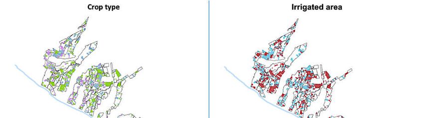
Water 2018, 10, x FOR PEER REVIEW                                                                              4 of 20

      observed an increased frequency of heavy rainfall events alternated with longer periods of severe
      droughts characterizing dry irrigating seasons.
            The case study region is selected because its decision process for water management is
      representative
Water 2018, 10, 1141   of other WAs located in Mediterranean countries where climate uncertainty strongly4 of 20
      affects decisions for land and water allocation before and during the irrigating season. Further, the
      prevalence of open-air canals in the water delivery network enhances both the challenges and the
mitigated    by the sea
      potentialities      influence
                      of ICTs       in the
                               adoption  at northeastern
                                            the WA level.part.   Droughtthe
                                                           Accordingly,   events  are frequent
                                                                             technical           in summer
                                                                                       constraints   of canals with
      require
variable         the WA
          intensity.      to anticipate
                       Although         decisions,
                                  the total amountmaking    forecasts
                                                     of rainfall      more
                                                                 appears to necessary  comparedmm),
                                                                            be stable (750–850      to similar
                                                                                                         in the last
      conditions    with pressurized  pipe  networks. Finally, the CBR’s management    board  is  considering
few years a change of the rainfall distribution was recorded. Specifically, it was observed an increased
      adopting a new information service named MOSES, developed in the framework of the MOSES
frequency    of heavy rainfall events alternated with longer periods of severe droughts characterizing
      H2020 European project, recently introduced to fulfil WA requirements.
dry irrigating seasons.

                      Figure 1. Case study region (source: own elaboration on data provided by CBR).
                  Figure 1. Case study region (source: own elaboration on data provided by CBR).
            The predominant water source for irrigation is the Canale Emiliano Romagnolo (CER). The CER
      The open-air
      is an  case studycanalregion
                              which diverts    part of because
                                       is selected       the water from   the Po river
                                                                     its decision        to several
                                                                                      process    forirrigation  boards. The
                                                                                                        water management         is
      irrigating season   generally   takes  place   from   May  to  September.    However,    due
representative of other WAs located in Mediterranean countries where climate uncertainty strongly    to yearly variability, it
      can
affects    be anticipated
         decisions          or delayed.
                      for land   and waterPeaksallocation
                                                  in water delivery
                                                               beforeare andinduring
                                                                               June andtheJuly, when crop
                                                                                             irrigating      water demand
                                                                                                           season.   Further, the
      is higher. The operational unit at which decisions on water management are taken is the irrigation
prevalence of open-air canals in the water delivery network enhances both the challenges and the
      district. The basin of the CBR includes 81 irrigation districts located in a plain area. The average
potentialities of ICTs adoption at the WA level. Accordingly, the technical constraints of canals require
      irrigated area is 68 ha per district and the average length of the water delivery network is 6 km per
the WA    to anticipate
      district. To verify decisions,
                           the usability making
                                           of MOSES forecasts    more
                                                          services,     necessary
                                                                    the WA    decided compared
                                                                                        to narrowto     similar
                                                                                                     down        conditions
                                                                                                            the scope  of the with
pressurized     pipe   networks.      Finally,   the    CBR’s   management          board   is considering
      investigation to a sub-group of its districts. Specifically, the WA selected only 32 of the 81 districts  adopting    a new
information     service   named      MOSES,      developed       in   the framework       of  the    MOSES
      covering an area of 18,845 ha, out of which 6012 ha are cultivated land. Such districts have the        H2020    European
project,  recently
      common         introduced of
                 characteristics    to afulfil WAwater
                                          unique      requirements.
                                                             source (represented by the CER) that is managed on
      demand,
      The        and of an water
            predominant       irrigation
                                     sourcenetwork     characterized
                                               for irrigation     is thebyCanale
                                                                            open-air   canals. On
                                                                                    Emiliano          average, the
                                                                                                Romagnolo          irrigated
                                                                                                                (CER).  The CER
is an open-air canal which diverts part of the water from the Po river to several irrigationthat
      land  is around   2878  ha, 48%    of the cultivated    land  (Figure   2). This area  corresponds    to the land    boards.
      can be irrigated in conditions of average operational capacity of the water supply network. However,
The irrigating    season generally takes place from May to September. However, due to yearly variability,
      in regular seasons, the network reaches its maximum operational capacity when it satisfies the
it can be anticipated or delayed. Peaks in water delivery are in June and July, when crop water demand
      demand from irrigated crops for around 3741 ha (130% of the average operational capacity). On the
is higher.   The operational unit at which decisions on water management are taken is the irrigation
      other hand, in dry seasons, the water supply network reaches its minimum operational capacity and
district.
      the WA isbasin
           The    able toof  the CBR
                          satisfy        includes
                                   the demand     for 81   irrigation
                                                       irrigation        districts
                                                                   for around   2014located
                                                                                      ha (70%in of athe
                                                                                                      plain  area.
                                                                                                        average     The average
                                                                                                                 operational
irrigated
      capacity). Despite the fluctuations in rainfall patterns, the land use tends to be constant where is
            area  is 68  ha  per  district   and   the    average   length    of  the water    delivery    network      6 km per
                                                                                                                      winter
district. To verify the usability of MOSES services, the WA decided to narrow down the scope of the
investigation to a sub-group of its districts. Specifically, the WA selected only 32 of the 81 districts
covering an area of 18,845 ha, out of which 6012 ha are cultivated land. Such districts have the common
characteristics of a unique water source (represented by the CER) that is managed on demand, and
of an irrigation network characterized by open-air canals. On average, the irrigated land is around
2878 ha, 48% of the cultivated land (Figure 2). This area corresponds to the land that can be irrigated in
conditions of average operational capacity of the water supply network. However, in regular seasons,
the network reaches its maximum operational capacity when it satisfies the demand from irrigated
crops for around 3741 ha (130% of the average operational capacity). On the other hand, in dry seasons,
Water 2018, 10, 1141 5 of 20
the water supply network reaches its minimum operational capacity and the WA is able to satisfy
the demand for irrigation for around 2014 ha (70% of the average operational capacity). Despite the
Water 2018, 10, xin
fluctuations FOR PEER REVIEW
rainfall patterns, the land use tends to be constant where winter crops are 5 of prevailing
20
(i.e., wheat, barley and meadow), followed by perennial crops (i.e., alfalfa, orchard, vineyard) and
crops are prevailing (i.e., wheat, barley and meadow), followed by perennial crops (i.e., alfalfa,
summer crops (i.e., maize and sorghum). The irrigation activity is centered around maize, orchard,
orchard, vineyard) and summer crops (i.e., maize and sorghum). The irrigation activity is centered
vineyard and horticulture;
around maize, winter
orchard, vineyard andcrops are generally
horticulture; winternot irrigated,
crops whilenot
are generally other crops while
irrigated, such as sugar
beet and alfalfa are occasionally irrigated.
other crops such as sugar beet and alfalfa are occasionally irrigated.
Figure 2. Land use in the case study region (source: own elaboration on data provided by CBR).
Figure 2. Land use in the case study region (source: own elaboration on data provided by CBR).
3.2. Management Systems and Information Requirements
3.2. Management Systemsseason,
Before the irrigating and Information Requirements
the WA decides the amount and allocation of yearly concessions to
cultivate annual irrigated crops. Concessions to irrigate permanent crops are granted for the whole
Before the irrigating season, the WA decides the amount and allocation of yearly concessions to
lifespan of the plantation. The decision for the amount of yearly concessions to irrigate is taken at the
cultivate annual irrigated crops.
time of seeding/transplanting annual Concessions to irrigate
irrigated crops, usually permanent crops arethe
in April. Typically, granted
WA forbidsfor the whole
lifespan of the plantation. The decision for the amount of yearly concessions
concessions to the latest applicants if the demand for concessions exceeds the average operational to irrigate is taken at
the time of
capacity ofseeding/transplanting
the supply network (6012 annual irrigated
ha). Under crops, usually
conditions in April.
of uncertainty Typically,
regarding the WA forbids
the rainfall
concessions
pattern of thetoupcoming
the latestseason,
applicants if the demand
this decision is the bestfor concessions
compromise exceeds
between the average
releasing concessions operational
to the maximum or to the minimum operational capacity of the supply network.
capacity of the supply network (6012 ha). Under conditions of uncertainty regarding the rainfall During the irrigating
season of
pattern andthein upcoming
each sector season,
of the agricultural
this decisionregion supplied,
is the the WA has to
best compromise plan with
between some advance
releasing concessions to
(i.e., one week) whether to deliver water to a sector or
the maximum or to the minimum operational capacity of the supply network. Duringnot. This is typically the case of surface
the irrigating
irrigation networks supplying water to an extended agricultural region. In such conditions,
season and in each sector of the agricultural region supplied, the WA has to plan with some advance
variations in the flow of water downstream of the network occurs with some delay with respect to
(i.e., one week) whether to deliver water to a sector or not. This is typically the case of surface irrigation
upstream variations in water flow. Thereby, under uncertain weather conditions, WAs usually decide
networks
to supply supplying
water on thewater tofixed
basis of an extended
flow ratesagricultural
varying withregion. In such
the season, conditions,
consistent with thevariations
average in the
flow of water downstream of the network occurs with
climatic condition of the region and with the amount of concessions provided. some delay with respect to upstream variations
in water Under this framework, the WA is considering the possibility of using the MOSES service towater on
flow. Thereby, under uncertain weather conditions, WAs usually decide to supply
the basis of
improve its fixed
capacityflow rates varying
to condition and towith thethe
satisfy season,
demand consistent
for waterwith the average
to irrigate. climatic
Specifically, the WAcondition of
is interested
the region and inwith
knowing the average
the amount weather conditions
of concessions provided. for the upcoming season at the time of
seeding/transplanting
Under this framework, and short-term
the WAforecasts about irrigation
is considering requirements
the possibility in each
of using thesector
MOSES of the
service to
region served by the WA during the irrigating season. The first piece of information
improve its capacity to condition and to satisfy the demand for water to irrigate. Specifically, the might influence
the WA’s decision on providing concessions to cultivate irrigated crops, reducing the risk of making
WA is interested in knowing the average weather conditions for the upcoming season at the time of
wrong choices. If a dry season is forecasted, the WA might decide to limit the number of concessions
seeding/transplanting and short-term forecasts about irrigation requirements in each sector of the
to the minimum operational capacity of the supply network. Otherwise, if a regular season is
region served
forecasted, thebyWA the WAset
could during the of
the limit irrigating
concessions season.
to theThe first piece
maximum of information
capacity of the network.mightTheinfluence
the WA’s decision on providing concessions to cultivate irrigated crops,
second piece of information would allow the WA to know whether to deliver water in each sector of reducing the risk of making
wrong choices.
the network If a dry
enough season istoforecasted,
in advance take timely the WAadjusting
action, might decidewater to limit
flows thethe
with number
demand. of concessions
Thus, to
Water 2018, 10, 1141                                                                              6 of 20

the minimum operational capacity of the supply network. Otherwise, if a regular season is forecasted,
the WA could set the limit of concessions to the maximum capacity of the network. The second piece
of information would allow the WA to know whether to deliver water in each sector of the network
enough in advance to take timely action, adjusting water flows with the demand. Thus, this additional
piece of information might influence the WA’s decisions on changing the management of the supply,
improving the efficiency of the supply network. However, because of technical constraints, the WA
must guarantee a threshold of minimum flow in the main canal for each district to allow an even water
distribution. This condition does not allow the WA to effectively manage water supply volumes and
limits its capacity to save water when the demand for water is low.

3.3. Usability of the MOSES Information Service
      MOSES provides spatially-detailed information to WAs both before and during the irrigating
season. In the first case, the information provided is a seasonal forecast of weather conditions and
crop water requirements. In the second case, MOSES delivers a daily seven-day forecast of crop
water requirements and weather forecast. To produce such information, MOSES combines crop
maps determined with satellite images, crop transpiration models, climate data and weather forecast
information as inputs. Specifically, with crop maps, crop water requirements are estimated and
forecasted in each plot using crop models with input from climate data and weather forecasts.
      As seen in the previous section, MOSES predictions before the irrigating season are likely to be
used to manage yearly concessions to irrigate. In the current conditions, the WA fixes concessions to
irrigate to the average operational capacity of the supply network. With MOSES services, if a dry season
is forecasted, the WA would limit the number of concessions to the minimum operational capacity.
Otherwise, in view of a regular season, it will release more concessions up to the maximum operational
capacity. Hence, the decision due is binary: to limit concessions to the maximum operational capacity
or to the minimum operational capacity of the water supply network. The benefits generated are:
avoided drought losses if the dry season occurs or higher agricultural revenues in the case of a regular
season. Nevertheless, information is not perfect, and two types of errors can emerge:

1.    the wrong prediction of a regular season: the WA receives a message specifying a regular season
      will emerge, but eventually the season will be dry;
2.    the wrong prediction of a dry season: the WA receives a message specifying a dry season will
      emerge, but eventually the season will be regular.

     The above errors lead to higher or lower concessions than the ones actually possible, causing a
sub-optimal use of land. If the number of concessions exceeds the contingent capacity of the WA, as a
consequence of error 1, farmers would experience a loss due to the difference between the average
income of rain-fed crops and irrigated crops with no irrigation water availability. It can be expected
that rain-fed crops have a higher comparative performance in terms of income in the case of low or no
irrigation water availability. If the number of concessions is below the capacity of the WA as in the
case of error 2, farmers would experience a loss due to the difference between the average income of
irrigated crops with fully available water and rain-fed crops.
     MOSES forecasts during the irrigation season are likely to be used to support decisions on water
allocation too. Due to the fixed water flows and technical thresholds, water allocation decisions are
binary: to deliver water to a district or not. Such a decision is repeated daily during the irrigating
season for each irrigation district. Compared to the current condition where the WA delivers water to
districts disregarding the demand, predictions of crop water requirements could support decisions on
water allocation during the irrigating season. The benefits generated by this piece of information are:
saving water, lowering supply costs, allocating water efficiently and softening damages in dry periods.
Here again, the provided information is not perfect, and two type of errors can emerge: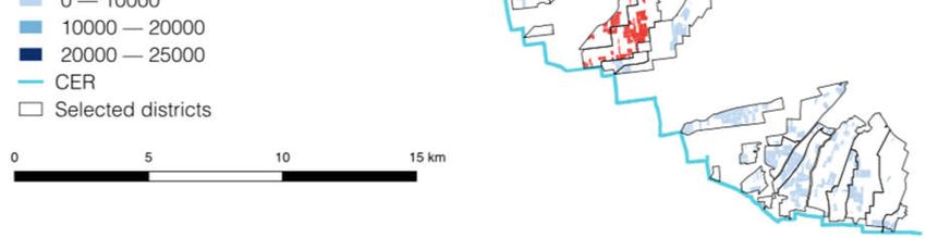
Water 2018, 10, 1141                                                                                                           7 of 20

1.       the wrong prediction that water requirements are above zero: the WA receives a message
         specifying that water for irrigation is needed in a specific sector of the network, but eventually
         water for irrigation is not needed;
2.       the wrong prediction that water requirements equal zero: the WA receives a message specifying
         no water demand for irrigation in a specific sector of the network, but eventually water for
         irrigation is needed.

      The above errors lead, respectively, to water flow or no water flow in sectors where no water is
     Water 2018, 10, x FOR PEER REVIEW                                                                                 7 of 20
needed and water is needed. This causes a sub-optimal use of water, where the first error leads to
water The
        waste   (measured
            above   errors lead,byrespectively,
                                     the amounttoofwater water     actually
                                                                flow           distributed
                                                                       or no water   flow in in  the sector)
                                                                                              sectors  where no with
                                                                                                                   waterunnecessary
                                                                                                                            is
supply
  neededcosts.    The second
           and water              error
                         is needed.    Thisleads   to damaged
                                              causes  a sub-optimal  irrigated
                                                                          use of crops
                                                                                 water,because
                                                                                         where the of first
                                                                                                       missing
                                                                                                             errorwater
                                                                                                                   leads to deliveries
  waterwater
when     wastefor(measured
                   irrigation  byisthe   amountneeded
                                     actually      of water   actually distributed
                                                            (difference     between thein the  sector) income
                                                                                           average      with unnecessary
                                                                                                                 of irrigated crops
  supply
with      costs. The
      irrigation   andsecond     errorcrops
                          irrigated      leads with
                                                to damaged     irrigated crops because of missing water deliveries
                                                      no irrigation).
  when   water   for  irrigation   is  actually   needed    (difference
      The whole decision process is represented in the decision            between thetreeaverage
                                                                                           of Figureincome     of irrigated
                                                                                                        3. Decision      alternatives
  crops with irrigation and irrigated crops with no irrigation).
branch from square nodes; the probabilities of uncertain events branch from round nodes and
       The whole decision process is represented in the decision tree of Figure 3. Decision alternatives
consequences of actions in state of the world are expressed in terminal nodes with prisms. In the
  branch from square nodes; the probabilities of uncertain events branch from round nodes and
two  decision time steps (before and during the irrigating season), information is provided through a
  consequences of actions in state of the world are expressed in terminal nodes with prisms. In the two
message.    This steps
  decision time    might(before
                             causeand a revision
                                            during ofthethe   WA’s beliefs
                                                          irrigating    season),depending
                                                                                  informationonis the   expected
                                                                                                    provided         consequences
                                                                                                                through      a
associated   withmight
  message. This      eachcause
                             message       content
                                    a revision        and
                                                  of the    on the
                                                         WA’s          accuracy
                                                                  beliefs          of the
                                                                           depending    on ICT.   The whole
                                                                                            the expected         decision process
                                                                                                            consequences
isassociated
   divided in    two
              with      decision
                     each   message time    stepsand
                                        content     (separated      in Figure
                                                       on the accuracy           3 by
                                                                            of the ICT.the
                                                                                         Thehorizontal    red dashed
                                                                                              whole decision     process is line) with
  divided
two        in two decision
     sequential                time steps (separated
                    binary decisions:          to releaseinconcessions
                                                              Figure 3 by the to horizontal
                                                                                 the maximum  red dashed    line) with
                                                                                                    operational          two
                                                                                                                     capacity     or to
  sequential  binary    decisions:    to  release  concessions     to  the maximum      operational
the minimum operational capacity of the water supply network and to deliver water to a district or     capacity   or  to  the
  minimum
not.         operational
     The decision      madecapacity       of the water
                               in the second       step supply    networkby
                                                         is influenced        and
                                                                                thetoexpected
                                                                                      deliver water   to a districtof
                                                                                                 consequences        orthat
                                                                                                                         not. decision
  The decision made in the second step is influenced by the expected consequences of that decision
during the irrigating season and by the accuracy of the messages provided before the irrigating season.
  during the irrigating season and by the accuracy of the messages provided before the irrigating
That implies a strict dominance of the accuracy of the messages provided in previous time steps on
  season. That implies a strict dominance of the accuracy of the messages provided in previous time
subsequent     ones. ones.
  steps on subsequent

                 Figure 3. Decision process of MOSES adoption by the CBR (source: own elaboration).
               Figure 3. Decision process of MOSES adoption by the CBR (source: own elaboration).
     4. Methodology and Empirical Application

     4.1. Definition of the Model
          The methodology adopts a simplified decision model to represent the decision-making process
     of the case study WA to select the best alternative among a set of actions upon receiving new
     information. The model assumes that a WA is managing water procurement and supply for a given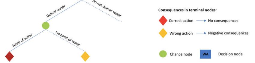
Water 2018, 10, 1141                                                                                 8 of 20

4. Methodology and Empirical Application

4.1. Definition of the Model
      The methodology adopts a simplified decision model to represent the decision-making process of
the case study WA to select the best alternative among a set of actions upon receiving new information.
The model assumes that a WA is managing water procurement and supply for a given agricultural
region and that the WA must plan some actions in advance during two different inter-correlated
decision time steps. The first decision step is supposed to be at the time of seeding/transplanting,
far in advance to the irrigating season, and involves the decision (action): release concessions to the
minimum/maximum operational capacity of the supply network. Such a decision is conditioned by
the WA’s expectation about the state of the world (state, from now on): dry/regular season. The second
decision step is supposed to be at the time of supplying water for irrigation and involves the decision:
deliver/do not deliver water to irrigation districts. Such a decision is conditioned by the WA’s
expectation about the state: need/no need water for irrigation. In chronological order, the first decision
influences the second. Thus, the usability of such information is then dependent on the accuracy of the
messages provided by the information service in both decision steps and on the stakes in the decisions,
contributing to determining the expected consequences of using the information. In the following
section, we provide an analytical representation of the decision process, both in case of un-informed
decisions and ICT-informed decisions. In the latter case, in each decision time step, a new piece of
information is provided by a message.
      The decision model described before represents a decision process taking place in conditions of
uncertainty. In the first place, we assume that the decision process involves a set of actions, X, and a set
of states, S. The combination of the possible actions with the possible states determines the associated
consequences, c x,s , measured in terms of economic payoff of the decision, v(c x,s ). The subscript x
denotes a specific action among the set of possible actions and the subscript s denotes a specific
state among the set of possible states, where x ∈ X and s ∈ S. For example, the consequence of not
limiting yearly concessions for irrigable areas in a regular season is drought losses, and the associated
payoff is the economic estimation of such losses. Thus, the actions taken by the WA have uncertain
consequences determined by the probability of occurrence of upcoming states, πs . In our case, the
probability coincides with the climate-relative frequency of the event. Assuming the WA is acting
rationally, it will base the choice of an action on the concept of Expected Value (EV) maximization. The
EV of an action depends on the probability of the different states and on the payoff of the set of possible
actions under the different states of the world [21]. With no information service, the maximization of
the EV is obtained by the following Equation (1):

                                        max EV ( x, πs ) =
                                        (x)
                                                             ∑ πs v(cx,s )                              (1)
                                                              s

     In the case of ICT adoption, the WA can receive a message, µ, among a set of messages, M (µ ∈ M).
The probability of receiving message µ is identified as πµ , which is measured as the frequency of
that message relative to all messages delivered by the ICT. Messages provide information regarding
the emerging state of the world. For example, a message can specify that a dry season will occur.
Messages might modify the WA’s information environment, altering the expectations associated to
the upcoming state of the world. The extent to which the WA reviews this prior expectation follows
the Bayes Theorem and is measured by the probability of state occurrence conditional to the message
received, πs|µ , also known as posterior probability:

                                                   jsµ
                                    (
                                        π µ| s ≡   πs
                                                                          π µ| s
                                                   jsµ   ⇒ π s |µ ≡ π s                                 (2)
                                        π s |µ ≡   πµ
                                                                          πµ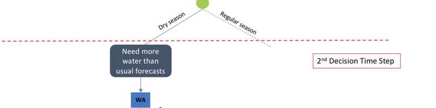
Water 2018, 10, 1141                                                                                                         9 of 20

where πµ|s is the probability of receiving message µ, conditional to the emergence of state s, and jsµ is
the joint probability of state s and message µ, also known as the hit rate [18]. This is measured in a
likelihood matrix by the frequency of correct messages on all messages delivered by the ICT. As can be
noticed, the higher the hit rate of the ICT, the higher the extent to which the WA will revise its prior
expectations. This implies that, by means of the accuracy of the ICT, the WA revises its beliefs about
a state’s occurrence after receiving a message. This in turn will have an effect on expectations about
decision outcomes with direct consequences on the choice of actions, allowing the WA to identify a new
optimal action. The EV of this action after receiving a message is determined by the sum of payoffs
weighted by the unconditional probability of the message and the respective conditional probability
of the states.  Considering
        Water 2018, 10, x FOR PEER an ICT delivering multiple messages, the maximization of the9 ofEV
                                   REVIEW                                                                20 will be
as follows:
        sum of payoffs weighted max     by the   x, πs|µ = ∑
                                            EV unconditional   πµ ∑ πsof
                                                             probability     the message and the respective
                                                                         |µ v ( c x,s )                          (3)
         conditional probability of (the
                                     x ) states. Considering
                                                          µ an ICT
                                                               s   delivering multiple messages, the
         maximization of the EV will be as follows:
     Now, consider a simplified version of the model described above, with only two alternative
states (s1 and s2 ), two alternative actions          ,(x1| and
                                                              = x2 ) and one   |   ( decision
                                                                                      , )         time step. This (3)    model can
                                            ( )
be represented through the diagram in Figure 4. Payoffs in each state are measured vertically and
probability Now,     consider ahorizontally,
               is measured       simplified version    of thefrom
                                                 ranging       model    described
                                                                     zero    to oneabove,     with only two alternative
                                                                                        in a bi-directional       segment. Since
         states ( and ), two alternative actions ( and ) and one decision time step. This model can be
states are alternative, meaning that one excludes the other, probabilities of state occurrence are
         represented through the diagram in Figure 4. Payoffs in each state are measured vertically and
complementary       (π + π2 = 1).
         probability is1 measured
                                       Hence, a point along the segment represents both probabilities. In the
                                    horizontally, ranging from zero to one in a bi-directional segment. Since
diagram,    the  blue  line  joining   v
         states are alternative, meaning (cs1x1
                                            that) and   v(cs2x1 ) the
                                                  one excludes     is the    weighed
                                                                         other,            average
                                                                                  probabilities       of payoffs
                                                                                                 of state  occurrence     action x1 .
                                                                                                                      forare
This linecomplementary
           expresses the( EV  + for=that   actiona as
                                      1). Hence,        a function
                                                    point   along theof    probabilities.
                                                                        segment    representsSimilarly,     the pinkInline,
                                                                                                both probabilities.      the which
joins v(cdiagram,  thevblue
          s2x2 ) and        line
                       (cs1x2    joining ( the) EV
                              ), represents         andof (action) isx2the  weighed
                                                                         . For   a givenaverage  of payoffs
                                                                                           probability,   theforEVaction
                                                                                                                     of the.optimal
action isThis line expresses
           displayed   by thethe  EV for that
                               vertical       actionfrom
                                          distance   as a function
                                                             a pointofinprobabilities.
                                                                           the horizontal Similarly, the pink
                                                                                               segment          line, which to the
                                                                                                          of probabilities
         joins (      ) and (        ), represents the EV of action . For a given probability, the EV of the
higher EV function between x1 and x2 . Taking into account an information service that can generate
         optimal action is displayed by the vertical distance from a point in the horizontal segment of
two alternative     messages
         probabilities
                      to the    (µ1 and
                           higher          µ2 ), either
                                       EV function         messageand
                                                       between           will lead
                                                                               . Takingto ainto
                                                                                             vector   of posterior
                                                                                                account   an informationprobability,
πs|µ = service    , πcan
            πs1|µthat        . The two
                       s2|µgenerate linealternative
                                         joining the     EV of(μtheand
                                                    messages          optimal    action
                                                                         μ ), either      if µ1will
                                                                                     message    is received     and if µ2 is
                                                                                                    lead to a vector
         of posterior  probability,     = (     ,      ). The line joining  the  EV  of the optimal
received, defines the EV of the message service. This is mathematically represented by the probability
                                      |       |      |                                                action if μ is
         received and if μ is received, defines the EV of the message service. This is mathematically
weighted average of payoffs. So, following Equation (3), the VOI is graphically represented by the
         represented by the probability weighted average of payoffs. So, following Equation (3), the VOI is
vertical graphically
         distance from     the line of the EV of the message service to the EV of the best un-informed action
                      represented by the vertical distance from the line of the EV of the message service to the
(green segment     in Figure
         EV of the best        4). action (green segment in Figure 4)
                         un-informed

           Payoffs in State 1                                                                      Payoffs in State 2

                                                                                                             v(cs2x2)

           v(cs1x1)    x1

                                                                VOI

                                                                                                             Probabilities
                                 πs1|µ1                        πs1                              πs2|µ2
                                                               πs2                                           v(cs2x1)

                            x2

           v(cs1x2)

               Figure 4. Graphic representation of the decision model after receiving a new message (source: own
      Figure 4. Graphicfrom
             elaboration representation
                             [16]).     of the decision model after receiving a new message (source: own
      elaboration from [16]).
               Finally, we take into account a decision problem involving decision time steps. Decision steps
         are identified as sequential decisions occurring during time (i.e., before and during the irrigating
         season). For each decision step, t, there are independent actions, , messages, μ , and states, . The
         set of possible consequences is obtained with the combination of actions and states in each time step,
         t, for the subsequent combination until the final decision step. In other words, the combination of
         actions, states and decision steps allows for the identification of the range of final outcomes of the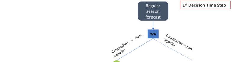
Water 2018, 10, 1141                                                                               10 of 20

     Finally, we take into account a decision problem involving decision time steps. Decision steps are
identified as sequential decisions occurring during time (i.e., before and during the irrigating season).
For each decision step, t, there are independent actions, xt , messages, µt , and states, st . The set of
possible consequences is obtained with the combination of actions and states in each time step, t, for
the subsequent combination until the final decision step. In other words, the combination of actions,
states and decision steps allows for the identification of the range of final outcomes of the decision
process. Since decision steps, states and messages are independent, the expected value maximization
problem can be reformulated as it follows:
                                                       "              #

                                                  ∏ ∑ πµt ∑ πst|µt

                        max EV xµt , πst|µt =                             v c xµt ,   st               (4)
                        ( xµt )                    t       µt   st

      Hence, during time in the decision process, the final choice of actions made by the WA depends
on the accuracy of the messages received until the final decision step. This way, a lack of accuracy in
the first messages has a multiplier effect in determining the expected consequences of sub-sequential
actions. Finally, in each decision step and for each message received the WA, the WA seeks the optimal
choice of actions among those available. This is done through the identification of the optimal informed
          ∗ ) achieving the highest EV given the states that can emerge and their relative posterior
action (xµt
probabilities. The same happens in un-informed conditions, where, given the prior probabilities of
states, the WA identifies the optimal un-informed action in each decision step (x0t  ∗ ). After optimizing

action choices, the VOI can be estimated as the difference between the EV from the sequence of optimal
informed actions given the messages received, and the EV of the optimal un-informed actions given
the prior information environment:

                                            ∗                   ∗
                                  VOI = EV xµt , πst|µt − EV ( x0t , πst )                             (5)

     As can be seen, the VOI of the ICT is positive only when the expected value of the best informed
decision is higher than the EV of the best uninformed decision. This happens when posterior
probabilities of the states given messages are higher than their prior. Otherwise, messages would be
uninformative, not conditioning any appreciable change in the behavior of the WA.

4.2. Data Collection and Assessment Procedure
      The usability of the information service is dependent on the accuracy of the messages provided
by the information service itself and on what is at stake in the decisions. These elements contribute to
determining the expected consequences of using the information. The sources of information needed
to carry out the economic analysis are mainly based on: (1) information obtained by interviewing the
WA; (2) information provided by the MOSES service; (3) additional ancillary information.
      The first type of information is about the collection of primary data through an ad-hoc
questionnaire. The questionnaire includes sections on: (i) WA information requirements; (ii) irrigation
infrastructures (including details on water supply costs, efficiency of the supply system and on the
amount of water delivered in each sector/district of the network); (iii) land use and cropping patterns
(i.e. rain-fed and irrigated crop yields) and (iv) damages caused by extreme weather conditions
(probability of a drought, expected damages per crop categories). The questionnaire helped to build
the ICT informed decision model and to identify consequences of actions in states. With the joint use
of secondary economic data on prices and yields from public databases (RICA–Rete di Informazione
Contabile Agricola, 2017: http://rica.crea.gov.it/public/it/index.php) and information on land use,
damages, crop prices and costs and on water price and use, it was estimated that the economic payoff
associated to consequences of actions in states. To simplify the assessment procedure, impacts of the
decisions were estimated with the spatial limitation of the case study area.
Water 2018, 10, 1141 11 of 20
The second type of information is about the new data provided by MOSES before and during the
2017 irrigating season. These are mainly crop water demand seasonal and in-season forecasts. Such
data were provided with different spatial resolutions, then aggregated in functional management units
(sectors of the irrigation network). The collection of such information allowed us to build a complete
picture of the information environment which would have characterized the ICT-informed decision
process of the WA in 2017.
The third type of information collected was needed to assess the accuracy of MOSES services.
These are observed data in the form of: (i) aerial photos (provided by the WA); (ii) weather observation
(available from MOSES meteorologists) and (iii) observed crop water requirements. The collection
of such information is justified by the fact that the accuracy of the service is mainly dependent on
three sources of uncertainty, contributing to the accuracy of the messages provided by MOSES: (1) crop
maps; (2) water demand estimates, and; (3) forecasts. The accuracy of information was estimated from
the hit rate of the service, coming from the ratio between the number of correct messages of the overall
messages received by the WA. This ratio is a rough estimate of the probability of correctly predicting
current and upcoming states. Specifically: (1) by comparing MOSES crop maps with aerial photos
(provided by the WA), we calculated the probability that an irrigated crop mapped with MOSES
satellite images matches with an irrigated crop mapped with aerial photos; (2) by comparing MOSES
rainfall forecasts with rainfall observation, we calculated the probability that a forecasted rainfall
above the estimated crop water requirements matches with the observed rainfall above the estimated
crop water requirements. In addition, due to missing information, we assumed that, by comparing
MOSES estimates of irrigation requirements with measured irrigation requirements, the probability
that a positive irrigation requirement estimate (greater than zero) matches with a positive irrigation
requirement measured with soil moisture sensors. Each of the above comparisons and assumptions
contributed to the calculation of the probability of predicting a dry or a regular season before the
irrigating season and the probability of predicting water requirements above or below a threshold
value of 10 mm. This value is assumed to be the critical level influencing the amount of water to be
supplied for each sector of the irrigation network during the irrigating season.
Appendix A provide all the information needed to test the assessment methodology for the
estimation of the accuracy of information and the payoffs of the decision process.
5. Results
The estimation of the accuracy of the MOSES information was carried out by comparing MOSES
output with observed data, as described in the previous section. Results about the accuracy of the
messages provided through MOSES are displayed in the probability matrix of Tables 1 and 2. The
overall accuracy of each message is expressed by the probability to correctly detect the land use
multiplied by the probability to correctly predict if water requirements are above the 10 mm threshold.
As can be seen from the tables, the accuracy of the messages is not evenly distributed between states
and the crop classification appears to be less reliable than the forecast of water requirements.
Table 1. Probabilities to detect the land use.
MOSES Crop Classification
Irrigated Not Irrigated
Observed Data on Irrigated 0.66 0.41
Land Use Not irrigated 0.34 0.59
Source: own elaboration.Water 2018, 10, 1141 12 of 20
Table 2. Probabilities to predict water requirements.
MOSES Irrigation Forecast
Water Requirements Water Requirements
Above the Threshold Below the Threshold
Water requirements
0.80 0.06
Observed Data above the threshold
Water requirements
0.20 0.94
below the threshold
Source: own elaboration.
Water savings brought by the use of the forecast information are determined both in regular and
dry seasons. The variability of water savings is measured across time and is calculated by comparing
water requirement estimates with the water actually supplied to districts in 2017 (Figure 5). Water
savings and water use tend to show a parallel trend. This highlights the fact that higher water savings
are more easily achievable in periods with higher water use. In the first weeks of the irrigating season,
higher variability of water use can be found, with two peaks at week three and six. Such phenomena
are mainly due to the rain distribution in late spring, which is particularly variable in the case study
area. Further, at the beginning of the season, peaks in water demand are caused by early concessions to
irrigate. These are released to allow the seeding/transplanting of summer crops, which are extremely
sensitive to droughts in the first phenological stages. Finally, in dry season with water scarcity, lower
water savings are achievable because water demand tends to be equal to the water available.
Table 3 represents the payoff matrix expressing payoffs in each state action combination for both
decision steps. In the assessment, the impact of optimal decisions is estimated to be zero, since they
stand for the most suited management strategy given the climate conditions. Then, with reference
to the optimal decisions, losses are estimated for each sub-optimal state action combination. Great
variability in decision outcomes can be found because the same action has extreme consequences with
the emergence of a dry season or a regular season. For example, with wrong water allocation decisions,
great drought losses can emerge, or wrong land allocation causes sub-optimal use of resources with
negative impacts on farmers’ income.
By applying the model in Section 3, the accuracy of the ICT information is used to compute
the EV of each action whose payoffs are represented in Table 3. Then, the VOI is assessed as the
difference in expected decision outcome between the best decision process with information and
without information. Summing over the VOI assessed in each district, potential benefits of the
ICT-informed decision model are estimated to be 156,426 € for the irrigating season of 2017 and for all
32 districts examined (26.02 €/cultivated hectare/year). The spatial distribution of the VOI (Figure 6)
is highly variable. Some districts have a null benefit from the implementation of such technologies,
others have a very high benefit.in expected decision outcome between the best decision process with information and without
information. Summing over the VOI assessed in each district, potential benefits of the ICT-informed
decision model are estimated to be 156,426 € for the irrigating season of 2017 and for all 32 districts
examined (26.02 €/cultivated hectare/year). The spatial distribution of the VOI (Figure 6) is highly
variable.
Water Some
2018, 10, 1141 districts have a null benefit from the implementation of such technologies, others
13 have
of 20
a very high benefit.
Figure 5. Estimated
Figure waterwater
5. Estimated savings during
savings the irrigating
during season
the irrigating (source:
season own own
(source: elaboration).
elaboration).
Table 3. Payoffs of the decision model in the case study region (€).
Table 3. Payoffs of the decision model in the case study region (€).
States
s’1 s’2
States
s’’1 s’’2 s’’1 s’’2
x’’1 - s’1
−608,181 −252,155 s’2 −1,112,491
x’1
x’’2 −464,777 s”1 - s”2 s”1
−366,491 s”−252,155
2
Actions
x’’1 −252,155
x”1 -−1,112,491 −608,181 −-252,155 −860,336
−1,112,491
x’2 x’
x’’2 1 −366,491
x”2 −464,777
−252,155 - −366,491
−728,569 −252,155
-
Actions
Source: own elaboration; x’ 1 : x”1
concessions up −
to252,155
the max. −1,112,491
capacity of the -
network; x’ 2: −860,336 up
concessions
x’2
x”2 −366,491 −252,155 −728,569 -
to the min. capacity of the network; x’’ 1: do not deliver water in a district; x’’2: deliver water in a district;
Source:
s’1: dryown elaboration;
season; x’1 : concessions
s’2: regular season; s’’1up to theofmax.
: need capacity
water; of need
s’’2: no the network; x’2 : concessions up to the min.
of water
capacity of the network; x”1 : do not deliver water in a district; x”2 : deliver water in a district; s’1 : dry season; s’2 :
regular season; s”1 : need of water; s”2 : no need of water
Because the accuracy of information is estimated using inputs from only one irrigating season,
it was considered useful to run a sensitivity analysis. This method is frequently adopted in literature
for the estimation of ICTs [13]. By varying the accuracy of information in both decision steps, we
determined the VOI in each condition of the information environment. In detail, we built an index
named Quality of Information (QI), ranging from zero to one, expressing the probability of correctly
predicting events. It is determined by the average accuracy of the messages provided to the WA before
and during the irrigating season. The QI will be null when the posterior probability to correctly predict
events coincides with its prior. The opposite will occur in the case of perfect information; QI will
equal one. The graph in Figure 7 shows how the VOI is related to the QI by increasing the accuracy of
information of every message in the two subsequent decision time steps. As expected, by raising the
QI for both decision steps, we see a non-decreasing linear trend of the VOI. It reaches its minimum in
uninformed conditions (QI = zero) and its maximum with perfect information (QI = one), where the
WA is sure to make optimal decisions. The trend is linear because of the linear equation used to model
the VOI, which it is determined as the difference in EV between informed and uninformed decisions.
Kinks can be noticed in the trend of the VOI; these take place when a new piece of information is
introduced with the required accuracy to cause a belief revision. Accordingly, for each decision, there
will be a threshold in the accuracy of the message provided, under which the WA does not revise its
expectations about state occurrence. Above such a threshold, the WA revises its beliefs and perceives
benefits of the improved decision. In the second decision step (T2), we determined the VOI both
in case of perfect information at the first decision step (T1) (before the season) and no information
provision at T1. This choice is motivated by the fact that the overall decision outcome is affected by the
accuracy of information at both decision steps. In detail, water allocation decisions are influenced by
the expected consequences of that decision during the irrigating season and by the decisions on landYou can also read