FUEL EFFICIENCY AND THE PHYSICS OF AUTOMOBILES1
←
→
Page content transcription
If your browser does not render page correctly, please read the page content below
FuelEff&PhysicsAutosSanders

              FUEL EFFICIENCY AND THE PHYSICS OF AUTOMOBILES1

                                   Marc Ross,
    Physics Department, University of Michigan, Ann Arbor MI 48109-1120

Energy flows and energy efficiencies in the operation of a modern
automobile are expressed in terms of simple algebraic approximations.
One purpose is to make a car's energy use and the potential for
reducing it accessible to non-specialists with technical backgrounds.
The overall energy use depends on two factors, vehicle load and
powertrain efficiency. The former depends on speed and acceleration
and key vehicle characteristics such as mass. The latter depends on
heat-engine thermodynamic efficiency, and engine and transmission
frictions. The analysis applies to today's automobiles. Numerical
values of important parameters are given so that the reader can make
his or her own estimates. Various technologies to reduce the energy
consumption of automobiles are discussed.

The Need for More-Efficient Vehicles

     In the United States, the fuel economy of new automobiles
increased 60% from 1975 to 1982. In terms of barrels per day of oil,
this efficiency improvement is far larger than production from any
oil field. A reasonable estimate of the impact of this change on
today's petroleum consumption is obtained by applying the 60%
improvement, in average miles per US gallon or km per liter, to
today's driving. The result is a gasoline savings of 3.3 million
barrels per day in the US, more than half the total crude oil
production in the US of 5.8 million barrels per day.2 Fuel efficiency
is indeed a powerful way to help energy ends meet.3

     Since 1982, however, the fuel economy of new automobiles in the
US has stalled at an average test-value near 25 miles per US gallon4
and has even been declining (Heavenrich & Hellman 2003).
"Automobiles" refers here to passenger cars and light "trucks" under
4 tonnes, like "sport utility vehicles", minivans and pickup trucks.
The latter vehicles are in wide use in the US, and almost all, except
for full-size pickups, are used in exactly the same ways as passenger
cars. That is, few of these so-called trucks are ever driven with

1
  originally published in Contemporary Physics 38, no. 6, pp 381-394, 1997.
This version is updated in parts to 2004 and modified in parts.
2
  Annual Energy Review, Energy Information Administration, Tables 5.2 & 5.12c.
The estimate is 8.7*(1 - 1/1.60) = 3.3 mbd, where 8.7 is motor gasoline usage.
3
  This paper is written from a US perspective. In the US, fuel economies
were increased to their present levels by regulation. In many other
industrial countries, relatively high fuel taxes are, in part, responsible
for average fuel economies up to 25% higher than in the US.
4
  corresponding to 9.4 L/100 km

                                                                              1
FuelEff&PhysicsAutosSanders
different loads than cars or are driven off road. But they are not
regulated as cars in terms of energy, pollution, safety or taxes. A
major reason fuel economy has stalled is the increasing use of these
light trucks, whose fuel economy is typically poor. The other reason
is that most manufacturers regard the fuel economy standards as
ceilings, exploiting efficiency improvements for increased size and
performance at the same fuel economy. Meanwhile, driving is
increasing 2 to 3% per year. At this rate, US petroleum consumption
would double in about 3 decades. This open-ended dependence on
petroleum, largely imported, is a major motivation for developing
more-efficient vehicles. Emissions also provide a strong motivation.
First good news: Regulation of "criteria pollutant" emissions
has led to much cleaner vehicles in the last 30 years. In the US new
2004 vehicles are restricted to emit less than about 2% of their mid-
1960s grams/mile levels of hydrocarbons and nitrogen oxides, and less
than about 5% of pre-control CO emissions (so-called tier 2
standards)! Those are test levels; real-world emissions of these
pollutants were several times higher than the test-levels of the
1990s (Calvert et al. 1994, Ross et al. 1995). Taking into account
the growth in travel during this period, the decline in total
emissions from new automobiles since the mid 1960s may have been 80
to 90%. This reduction has been accomplished by breakthroughs in
catalytic chemistry and sophisticated controls, e.g, of the engine's
air-fuel ratio. This reduction has enormously improved health and the
simple enjoyment of our metropolitan areas. And while ambient air
quality is still not satisfactory in many cities, new automobiles may
not have an important role in that.
This good news is balanced by the bad news about greenhouse gas
emissions and global climate change. Mobile sources contribute about
one-third of the emissions of carbon dioxide in the US, and those
emissions are growing. Cleaning up the exhaust cannot reduce the CO2
emissions the way it does for the criteria pollutants. However, there
is a way to enable reductions in these emissions: increased vehicular
efficiency, or fuel economy.
In a sense, however, the strongest motivation for higher vehicle
efficiency is technological feasibility. Today's capability to
design and manufacture high-tech products is revolutionary, because
of new materials and new kinds of sensors based on microprocessors.
Manufacturers are now able to carry out routinely concepts only
dreamed of by the automotive pioneers of a century ago. If
individual buyers, or society, placed a high value on fuel
efficiency, it could be greatly improved at low cost. Let us explore
the possibilities.
Overview of the Formalism
The consumption of fuel energy by a vehicle depends on two
factors: 1) the vehicle load, the work or power involved in moving
the vehicle and operating its accessories, and 2) the energy-
efficiency of the powertrain (engine plus transmission).
2FuelEff&PhysicsAutosSanders
The powertrain efficiency is the product of the engine's
thermodynamic efficiency, ηt, the engine's mechanical efficiency, ηm,
and the transmission efficiency ε:
powertrain efficiency = Pload/Pfuel = ηt•ηm•ε (1)
where Pload is the vehicle load and Pfuel is the rate of consumption
of fuel in energy terms, both in kW. These quantities are all
functions of time, some of them sensitively. The vehicle load is the
powertrain output: the rate of increase in kinetic energy plus the
rate of energy loss in the air drag, tyre drag and accessories.
The thermodynamic efficiency is the fraction of fuel energy
converted to work within the engine:
ηt ≡ (Pfrict + Pb)/Pfuel (2a)
where (Pfrict + Pb) is total work, which consists of output or "brake"
work, Pb, and internal frictional work, Pfrict.5
The mechanical efficiency is the fraction of the total work that
is delivered by the engine to the transmission:
ηm = Pb/(Pb + Pfrict) (2b)
And the transmission efficiency is:
ε = Pload/Pb (2c)
except that the accessories are generally driven by the engine
without going through the transmission. The relationships are
different when the load is negative, in braking.
In the following I address conventional automobiles. I first
discuss vehicle load and the engine's thermodynamic efficiency,
including a brief listing of techniques for improving both of them.
I go on to discuss mechanical efficiency in more detail, with
numerical examples. Then I focus on the potential for improving the
mechanical efficiency. Finally, I summarize the overall potential
for improving fuel economy.
The spirit of the analysis is a physicist's, rather than that of
an engineer who is responsible for a vehicle's performance. I want
to describe the energy flows accurately enough for general
understanding and perhaps conceptual design, not for designing an
actual vehicle. The approach is to develop simple algebraic
expressions motivated by physical principles, in contrast to the now
pervasive analysis based on numerical arrays. Creating an energy
analysis in, hopefully, transparent terms should make the issues
5
"Thermodynamic efficiency", is not standard terminology. It's often called
"indicated" efficiency.
3FuelEff&PhysicsAutosSanders
accessible to non-specialists with technical background. Moreover,
with the named quantities introduced, it is easier to discuss the
important and interesting opportunities for efficiency improvement.
Energy Use by Today’s Vehicles
Vehicle Load. Neglecting minor effects, such as wind and road
curvature, the instantaneous load is (Gillespie 1992):
Pload = Ptyres + Pair + Pinertia + Paccess + Pgrade (3)
Here the terms are in kW, and are:
a) power overcoming rolling resistance: Ptyres ≈ CRMgv
where CR is the dimensionless coefficient of rolling resistance6, M
is the mass of the loaded vehicle, expressed in tonnes; and v is the
vehicle speed in m/s;
b) air drag: Pair = 0.5ρCDAv3/1000
where ρ is air density (roughly 1.2 kg/m3), CD is the dimensionless
drag coefficient, and A is the frontal area in m2;
c) inertia: Pinertia = 0.5M*[∆v2/∆t]
where M* is the effective inertial mass, about 1.03M, which includes
the effect of rotating and reciprocating parts,7 and [∆v2/∆t] is in
m2/s3;
d) vehicle-accessories (such as lights, radio, windshield wipers,
power steering and air conditioning): Paccess; and
e) grade: Pgrade = Mgvsinθ
where tanθ is the grade. The inertial and grade terms may be
negative.
The instantaneous output power required of the engine, Pb, is
Pload/ε, eq(2c). The engine output required in a 1995 Ford Taurus is
shown in Fig. 1 for: 1) sustained hill climbing on a 6% grade, the
highest grade normally found on a motorway or expressway, 2)
sustained driving at constant speed on level ground, and 3)
accelerating 3 mph/s, or almost 5 (km/h)/s, on the level. The graph
demonstrates that, as of 1995 US driving, 50 kW would suffice for
6
CR is often considered to have some v dependence.
7
Strictly speaking, this effective mass depends on the engine speed to
vehicle speed ratio. E.g., in low gears the ratio of the speed of
reciprocating parts to vehicle speed is relatively high.
4FuelEff&PhysicsAutosSanders
sustained driving in almost all situations, while the 105 kW or
higher capability provided in the average US car enables one to
accelerate rapidly at speeds well above most legal limits.8
For current "midsize" US cars, like the 1995 Ford Taurus, the
time-average load on the engine in the composite US urban and highway
driving cycle is Pb = 6.3 kW.9 In terms of gasoline 6.3 kW is
equivalent to 1.6 L/100 km or 0.67 US gallons per 100 miles. If it
weren't for the inefficiencies of the powertrain, the fuel economy
would be astonishingly good. Nevertheless, major fuel savings can
still be achieved by reducing the load, especially weight reduction.
Figure 1. Engine Power Requirements, 1995 Ford Taurus
Speed
……...(km/hr)…….
75 100 125
140
120 acceleration: 3mph/sec
(4.8km/h/s) on level
100
80
sustained 6% grade
60
40
20
cruise (level)
0
45 55 65 70 75 80
Speed (mph)
8
The figure is calculated using eq(3) with parameters given below. The
transmission efficiency is taken to be ε = 0.9, and engine speeds are
simplified in the calculation.
9
A driving cycle is a sequence of second-by-second vehicle speeds often
used to define vehicle performance for regulatory purposes.
5FuelEff&PhysicsAutosSanders
All the vehicle loads in eq(3) can be substantially reduced
through improved design, and (for weight and tyre loss) through
improved materials. We have studied current cost-effective
technologies, keeping the car's interior volume fixed. We found
that, relative to model-year 1990 averages, rolling resistance could
be reduced one-third, air drag one-quarter, and weight one-fifth
(DeCicco & Ross 1993). Based on that analysis for the composite US
driving cycle, the overall load can be reduced 27% relative to
vehicles like the one described in detail below.
This weight reduction is a simple estimate based on early 1990s
production-model designs; it grossly underestimates what could be
done with new materials, and new designs such as sandwich panels
(e.g. reinforced sheets with foam filling), small engines with high
power-to-displacement capability, and small transmissions such as the
double clutch automatics.
Unlike the efficiency of the powertrain there is no ultimate
limit to load reduction. Traveling in vehicles with steel wheels on
steel rails in an evacuated tunnel would involve very small loads
indeed. The situation is analogous to heating a building in cold
weather. The efficiency of the heating system is bounded by 100%
(ignoring heat pumps). But the load can be reduced as much as
desired. It is mediated by the building envelope, which could be
very thick, with high thermal insulation, and with a ventilation
system using excellent heat exchangers.
Thermodynamic efficiency of the engine. The ability of energy
to do work declines dramatically with combustion, i.e. when fuel
energy is converted to thermal energy. The elegant second-law
concepts of available work and lost work were introduced by Gibbs to
describe such situations (AIP 1974), and applied to automobile
engines by Keenan and others (Keenan 1948). Briefly: while high-
quality forms of energy can, in principle, be converted entirely into
work, thermal energy cannot. The available work content of thermal
energy is the maximum work that could in principle be done in
particular surroundings, such as the neighboring air at a given
temperature. Decreases in available work associated with
irreversible processes like combustion are counted as lost work.
While the escape of gas from confinement at high pressure is the most
commonly cited example of irreversibility, combustion is another
excellent example. The lost work that results is large.
Why not use a technology which directly converts a fuel's
chemical energy into work? A fuel-driven battery, or fuel cell, does
so. It converts fuel to electricity without the intermediate step of
combustion; so its efficiency is not necessarily limited by the
second law to be much less than 100% (Kartha & Grimes 1994). But, at
present, fuel-cell technology is complicated and expensive. When it
becomes well developed, vehicle engines with thermodynamic
efficiencies over 50% should be achieved. In the meantime, we will
continue to use a less-sophisticated technology based on combustion.
6FuelEff&PhysicsAutosSanders
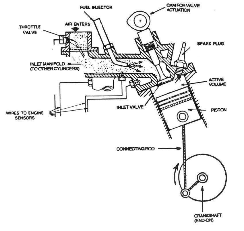
A typical modern spark-ignition engine's structure is
illustrated schematically in Fig. 2. Air is admitted to each
cylinder through two valves, a throttle common to all the cylinders
followed by an inlet (or intake) valve (or valves) for each. Fuel is
injected outside the cylinder near the inlet valve. In each full
cycle the piston goes through four strokes, and the crankshaft goes
through two revolutions. The strokes are illustrated in the
pressure-volume diagram, Fig. 3.
Figure 2. Sketch of a Cylinder and Intake System
The thermodynamic efficiency is broadly defined by eq(2a).
In particular, we take it to be the net work, relative to fuel input,
done by the compression-expansion strokes in the pressure-volume
diagram (Heywood 1988, Stone 1992). This work moving the pistons is
the area ∫pdV between the two upper curves in Fig. 3. And ηt is that
work as a fraction of the fuel energy.
In an Otto cycle, the compression and expansion strokes are
assumed to be adiabatic with a constant volume segment at the end of
each. The constant volume assumption is motivated by the slow rate
7FuelEff&PhysicsAutosSanders
of change in the active volume when the piston is near either end of
its motion. (See Fig. 2.)
Figure 3. Pressure-Volume Diagram (Four Stroke Spark Ignition Engine)
With an ideal gas as the thermodynamic fluid, the Otto cycle
efficiency is:
ηtI = 1 - 1/rcγ -1 (4a)
where rc is the compression ratio, Vmax/Vmin, and γ = cp/cv, as
discussed in many thermodynamics texts. (See, e.g., Zemansky &
Dittman 1981.) The thermodynamic efficiency increases with
increasing compression ratio and with increasing cp/cv. The latter
is related to the fraction of the thermal energy which goes into
translational motion of the gas molecules, i.e. to increased
pressure, as opposed to going into other molecular degrees of
freedom. Thus, stable diatomic molecules make a much better
thermodynamic fluid than complex molecules.
Texts on internal-combustion engines also discuss fuel-air-cycle
efficiencies, which still involve simplified cycles but use measured
thermodynamic properties of the gases, including effects of
dissociation at high temperature. The fuel-air cycle defined by the
outer envelope in Fig. 4 is still essentially an Otto cycle, with
constant volume ends and adiabats connecting them. The corresponding
efficiency, ηtFA, is calculated numerically as a function of rc and φ.
To a fairly good approximation:
ηtFA ≈ (1 - 0.25φ)ηtI (4b)
where φ is the fuel-air ratio relative to stoichiometric (Taylor
1985, v 1, p 95).10 The φ dependence represents the same issue of
10
At the stoichiometric fuel-air ratio, all the initial oxygen and fuel
could combine to form water and carbon dioxide.
8FuelEff&PhysicsAutosSanders
conversion of thermal energy into increased pressure as γ in eq(4a).
At the stoichiometric point, near which today's spark-ignition
engines normally operate, eq(4b) shows ηtFA ≈ 0.75ηtI. This loss of
efficiency occurs because the fluid is not an ideal gas and because
it doesn't have as large a value of cp/cv as air. Note that the
efficiencies (4a) and (4b) do not depend on engine operating point,
i.e. on speed and power.
The thermodynamic efficiency of an actual engine, ηt, is roughly
0.8 times that of the fuel-air cycle. The ways in which capacity to
do work is lost relative to the fuel-air cycle are: 1) heat loss,
heat escaping through the cylinder walls, 2) combustion-time loss,
delay of some combustion until well into the expansion stroke, 3)
exhaust blowdown, pressure release when the exhaust valve is opened
and, in addition, 4) fuel that is not burned within the cylinder.
The first three reductions in the area of the p-V loop are
illustrated in Fig. 4; heat loss is the largest. As for the fourth
loss, in engines controlled to operate stoichiometrically, unburned
fuel measured in the exhaust is 1 to 2% of the fuel input; but the
actual loss is higher because some burning takes place as the gases
leave the cylinder.
Figure 4. Pressure-Volume Diagram and Lost Work in the Compression and Power
Strokes
9FuelEff&PhysicsAutosSanders
Let the effective heat loss, relative to the heat released by
the fuel, be Q; and let losses (2)-(4) be approximately represented
by a constant efficiency, ηc.11 Then, for a real engine:
ηt = ηtFA•ηc(1 - Q) (4c)
In stoichiometric operation, typical values are ηc ≈ 95%, and Q ≈ 15%
(Muranaka et al. 1987). Q increases with decreasing cylinder size as
the surface to volume ratio increases; and it declines with declining
fuel-air ratio and increasing engine speed. The variation of Q is of
interest in exploring novel engines.
The best thermodynamic efficiency of conventional spark-ignition
gasoline engines is ηt ≈ 38%, relative to the lower heating value of
the fuel (or 35% relative to the higher heating value).12 For
comparison, boilers and steam turbines at electric power plants are
at most 40 percent efficient, and these engines are large, expensive,
and stationary. In new combined-cycle power plants, involving
recovery of work from the exhaust of the main combustion turbine, 50
percent efficiency is being achieved; and 60% performance is being
sought through truly elaborate schemes. (The latter efficiencies are
based on the higher heating value of fuel.)
I am making two points with these comparisons: First, cost
restricts automotive efficiencies; an automobile engine costs about
$20/kW, while the corresponding part of a power plant costs perhaps
$500/kW. Second, substantially increasing the thermodynamic
efficiency is difficult for any engine based on combustion; it can
never approach 100%.
The most practical measure to increase the thermodynamic
efficiency of automotive engines is to increase the fraction of heat
that increases the pressure, e.g. to have more of the thermodynamic
fluid be air or, in practical language, to use a lean fuel-air
mixture. In typical driving, ηt might be improved this way by as
much as a factor 1.15, e.g. ηt increasing to almost 44% from the 38%
characterizing the best conventional gasoline engines.
The most widely used lean-burn engine is the diesel, another
lean-burn engine is the new direct-injection stratified charge (DISC)
engine, which uses spark-ignition. In compression-ignition, or
diesel, engines the fuel has low volatility and is in the form of
small droplets after injection into the cylinder. Combustion
initiates on droplet surfaces at the high temperature and pressure.
The timing of combustion is controlled by the injection. Power
11
The heat loss is "effective" to the extent that it occurs at the
beginning of the power stroke, which most of it does. Thus the upper bold
curve in Fig. 4 is still essentially adiabatic except near minimum volume.
12
The lower heating value (LHV) is based on the water resulting from
combustion being a gas in the final state; the higher heating value (HHV)
is based on water as a liquid. In vehicles extraction of the heat of
condensation isn't practical so it is conventional to use LHV.
10FuelEff&PhysicsAutosSanders
output is controlled by the amount of fuel injected. There is no
throttle, the same amount of air being introduced in every cycle. At
low power, the fuel-air ratio is far below stoichiometric. But in
spite of their efficiency advantage, diesel engines have not caught
on for autos in the US because they have higher nitrogen oxide and
particulate emissions and they are heavier. Ten years ago, their
exhaust was apparent to anyone walking a main street in London.13
In order for the flame front to advance from the spark
throughout the cylinder in standard spark-ignition engines, the fuel
is vaporized, and mixed well with air. Power output is controlled
frictionally using the throttle, which creates a partial vacuum in
the inlet manifold (Fig. 2). At the same time the amount of injected
fuel is adjusted to obtain the desired fuel-air ratio. In the DISC
engine, making use of the control possible with direct injection,
turbulence and a spatially-varying fuel concentration enable the
combustion to be reliable at fuel-air ratios down to about one-third
stoichiometric.14 The DISC engine is in its infancy so it is early to
make judgments; but it appears to have a substantial advantage over
the diesel in the potential for emissions control, while it cannot be
quite as energy efficient. An alternative to achieving some of the
efficiency advantage of lean-burn engines at low power is to
recirculate much of the exhaust back into the cylinders (Lumsden et
al. 1997).
Another way to improve thermodynamic efficiency is to change the
shape of the pressure-volume diagram. One way is to adopt a longer
stroke so that the expansion is more fully exploited, but the
compression ratio experienced by the gases is kept the same by
keeping the inlet valve open in the initial stage (the Miller and
Atkinson Cycles now being introduced by Mazda and Toyota). While
higher compression ratios increase efficiency in principle, as shown
by eq(4a), they cause knock and involve increased friction. Yet
another possibility is to modify the engine fundamentally to recover
work from the hot exhaust gas in analogy with combined-cycle power
plants. Turbocharging offers such an opportunity, but the gain has
been modest so far; the primary purpose of turbocharging has been to
increase power at low engine speed (Gruden & Richter 1984, Shahed
2003, Institut Franç
ais du Petrole). Ambitious combined-cycle measures to save energy
have been adopted in some heavy-duty engines, but not yet in
automobiles. Finally, some improvement of ηt is also feasible
through insulating the cylinder walls; but in practice it probably
cannot be increased much in that way.
In summary, while today's best gasoline engines achieve a
thermodynamic efficiency of 38% and the best that could be done is
much less than 100%, it is practical to improve automobile engines to
13
For discussion of health effects see Health Effects Institute website.
14
In a quiescent fuel-air mixture the flame goes out for fuel-air ratios
less than about two-thirds stoichiometric. See discussion of flammability
limits in combustion texts. Achieving very low nitrogen oxide emissions
under these conditions is a major challenge for the technology.
11FuelEff&PhysicsAutosSanders
roughly 45%. Lean burn is the main line of development, but there
are other concepts which can even be combined with lean burn. The
challenge for lean-burn technology is to meet emissions standards
with room to spare, because those standards are in the process of
being tightened.
Mechanical efficiency. The mechanical efficiency, ηm, accounts
for the frictional losses in the engine. It is the ratio of work
output by the engine to the net work by the gases on the pistons in
the compression plus power strokes. Se eq. (2a) and(2b). There are
three engine frictions: 1) rubbing of metal parts, like piston rings
on cylinder walls, 2) gaseous friction, especially at the throttle
and valves, and 3) friction in the engine-accessories and their belt
drives (Heywood 1988, chapter 13).
The mechanical efficiency averages some 50 to 55% in the
composite US driving cycle, or about 45% if transmission losses are
included. Instantaneous ηm is very sensitive to the kind of driving,
near zero when the vehicle is coasting, braked or stopped, and high
when the load is high. At moderate engine speed and near wide-open
throttle ηm is about 85%. The power required in almost all driving
is far below the engine's maximum capability in today's vehicles, and
the resulting low ηm offers the easiest opportunity to increase fuel
economy, as discussed below.
The key to understanding efficiency is to "model the losses", in
this case the frictional work. A convenient notation is that of
"mean effective pressure":
mep ≡ 2000P/V N
Here P is power in kW averaged over an engine cycle, mep is in kPa, V
is the engine displacement or the swept volume Vmax - Vmin of each
cylinder times the number of cylinders, in liters, and N is engine
speed in rps. (The factor of 2000 is 2 from the number of
revolutions per 4-stroke cycle times 1000 L/m3.) The reason for
introducing mean effective pressures is that power roughly scales
with engine size and speed; thus mean effective pressures are roughly
the same for different engines and engine speeds.
The rate of frictional work in an internal combustion engine can
thus be written:
Pfrict = fmep V N/2000 (5a)
where fmep is "friction" mean effective pressure, cylinder pressure
averaged over the full four-stroke cycle. Similarly, the output
power can be written:
Pb = bmep V N/2000 (5b)
where bmep is "brake" mean effective pressure.
12FuelEff&PhysicsAutosSanders
Measurements of the rate of fuel use by internal combustion
engines show it to be essentially linear in the power output, except
near wide open throttle (WOT).15 This is known as Willans' line
(Roumegoux 1991, Ross 1994). An example of measurements supporting
this linear dependence is shown in Fig. 5. Here the y-axis is the
"fuel-equivalent" mean effective pressure which is defined as
(2000/VN)Pfuel.
At normal engine speeds, a satisfactory approximation for
friction in spark ignition engines is linear in bmep:
fmep = (fmep0 - c bmep) (6)
where fmep0 is the friction mean effective pressure at no load. The
negative bmep term is primarily associated with the throttling loss:
The throttle varies from almost closed at low power, to wide open, so
as the throttle valve is opened and power output increases, the
frictional loss at the throttle declines.
Figure 5. Measured Fuel Rate vs Power, Volkswagen 1.8 Liter Engine
40
35
1750 rpm
30
2500 rpm
25
20
15
10
5
0
0 2 4 6 8 10 12
Brake mep (bar)……..
15
Fuel use increases faster near WOT because of the practice of injecting
extra fuel, or making the mixture "rich", to improve performance and cool
the components.
13FuelEff&PhysicsAutosSanders
Here
c bmepWOT ≈ 60 kPa
the pressure drop into the inlet manifold at low power, a bit more
than 1/2 atmosphere; and, for engines which do not compress the
incoming air, bmepWOT ≈ 1000 to 1200 kPa. The linear approximation
for the fuel energy rate is then:
Pfuel = [fmep0 + (1-c)bmep] V N/(2000ηt) (7)
For good modern engines, typical values to use in eq(7) are:
fmep0 ≈ 160 kPa, and ηt = 0.38
for engine speeds near 30 rps (and they are not sensitive to V or N).
In the composite US driving cycle, excluding operations where no
power is delivered to the wheels, the average bmep ≈ 200 kPa. (Note
that it varies widely.) Thus a typical fuel-energy rate for a 2.0 L
engine is:
Pfuel = (160 + 0.94 200)2 30/(0.38 2000) = 27.5 kW, or
Pfuel/LHV = 27.5/44 = 0.62 g/s of fuel
Here LHV ≈ 44 kJ/g is the lower heating value of the gasoline. From
eq(6) we also see that the dimensionless slope in plots of the form
of Fig. 5 is (1-c)/ηt ≈ 2.5.
Overall engine performance. The overall efficiency of the engine
is:
η ≡ ηt•ηm = Pb/Pfuel (8)
In a first approximation, the efficiency ηt does not vary much
from engine to engine or with operating point (Ferguson 1986,
section 11.2); but fmep0 increases with engine speed (Yagi et al.
1991; Heywood 1988 chapter 13) and increases somewhat for small
engines (Ferguson 1986, section 11.1).
In Figure 6, a performance map is shown for a 2.7 L gasoline
engine, showing the brake specific fuel consumption:
bsfc ≡ (Pfuel/LHV)/Pb = 1/(η•LHV) (9)
The brake specific fuel consumption is commonly expressed as grams of
fuel consumed per kWh of output work. At the most efficient
operating point in Fig. 6, bsfc ≈ 255 g/kWh. The overall engine
efficiency at that point is thus η = 3600/(44•255) = 32.1%.
14FuelEff&PhysicsAutosSanders
Figure 6. Performance Map for a 2.7 Liter Spark Ignition Engine
Let us instead estimate η using the approximation eq(7), and the
parameters just given. Take the operating point with maximum
efficiency to be near 30 rps and Pb/PWOT = 0.74:
η = bmep•ηt/[fmep0 + (1-c)bmep]
= 740•0.38/[160 + (1 - 0.06)740] = 32.9%,
which is in satisfactory agreement with the value from Fig. 6. At
this operating point one also finds ηm = 0.86.
An engine's frictional work in a trip is roughly proportional to
the total number of revolutions made by the engine during the trip
and to the engine's displacement, based on the VN factor in eq(7).
Turning the engine off when the wheels are not powered reduces the
15FuelEff&PhysicsAutosSanders
engine-on time in the US urban driving cycle by almost 1/2 and the
number of revolutions by about 20%. Adopting an engine with only
half as much displacement reduces fmep by almost half. As we see
below, with good design, such opportunities could enable major
improvement in ηm with no or only minor sacrifice in performance.
A typical automobile’s energy consumption. There are three ways
to display the energy flows in vehicle operation (Table 1): 1)
Overall viewpoint: one explicitly describes all the losses within the
powertrain. 2) Work viewpoint: one explicitly describes all work
done against friction, but one allocates the "lost work", or
thermodynamic inefficiency, to the work categories. 3) Vehicle load
viewpoint: one explicitly describes only the vehicle loads,
allocating all the losses within the powertrain to the final loads.
TABLE 1.
ESTIMATED USE OF FUEL ENERGY BY A TAURUS IN THE COMPOSITE
US DRIVING CYCLE, FROM THREE VIEWPOINTS
(based on 100 units of fuel energy consumed)
viewpoint overall work v.load
vehicle loads
air drag 5 13 30
tyre rolling resistance 5 13 29
brakes 5 14 30
vehicle accessories 2 5 11
powertrain losses
engine “lost work” 62 NA NA
engine frictions 18 47 NA
transmission friction 3 8 NA
total 100 100 100
As shown in Table 1, the three major vehicle loads are
comparable in the US composite driving cycle (load viewpoint - right
column). (More realistically, in today's typical driving, speeds are
higher and the air drag term would be larger.)
The overall powertrain losses are shown in the left-hand column
of Table 1. The overall energy-efficiency, from fuel to wheels in
average driving, is the sum of the vehicle loads, i.e. 17 units out
of 100. This is essentially the product:
≈ ≈ 38%•53%•85% = 17% (10)
Here , the average automatic-transmission efficiency, is taken as
85%.16 One finds the overall 17% as the sum of the loads in the left-
hand column of Table 1, and ≈ 45% as the sum of the vehicle
loads in the central column. The 17% average powertrain efficiency
is powerful information. For example, it helps you to estimate how
16
Reasonable estimates of for urban and highway driving are 0.80 and
0.9, respectively. There is considerable variation; some analyses take
to be about 80% in the composite cycle, with in urban driving about
0.65. Manual transmissions are about 90% efficient in most driving.
16FuelEff&PhysicsAutosSanders
much more efficient an electric vehicle with the same vehicle load
might be. That exercise is left to the reader.
The thermodynamic lost work in the engine is 100 - 38 = 62%. As
shown in the overall perspective of Table 1, some 55% of the
remaining energy is work against powertrain friction. Thus, the work
against friction is 0.55•0.38 or 21% of the energy input, of which 18
points are engine friction and 3 transmission friction. This overall
perspective is illustrated in Figure 7. However, since the lost work
as a percentage is relatively difficult to change, the most
interesting perspective may be that of the work viewpoint (middle
column of Table 1).
Figure 7. Approximate Flows of Available Work: US Composite Driving Cycle
The reader who is interested can use the formalism, with the
help of a few parameters, to calculate fuel use by various vehicles
in various kinds of driving. Examples are carried through for
constant-speed driving and driving in the US driving cycles in the
Appendix.
Improving Mechanical Efficiency
As the work viewpoint in Table 1 shows, over half the fuel
energy in the composite driving cycle is used to overcome friction
within the engine and transmission. These losses could be greatly
reduced through changes broadly characterized as design.
17FuelEff&PhysicsAutosSanders
The Performance Challenges for New Designs. Before considering
design of a more efficient car, however, let's review vehicle-
performance characteristics which may interact with design choices.
There are three important measures of driving performance
characterized by times of minutes, a few seconds, and a fraction of a
second:
The first is maximum sustained power - for minutes - the
determinant of speed in a long hill climb. Substantially less power
than that of today's engines would do for today's typical midsize
car. For example, 50 kW would enable a midsize car to maintain 65
mph (105 km/h) up the 6% grade on the expressway west of Denver (Fig.
1 above). High speed on level ground, albeit not autobahn speed, is
less of a challenge.
The second is maximum transient power - for several seconds -
the determinant of acceleration capability in high-speed driving and
of 0 to 100 km/h acceleration time. This is where the maximum power
capability of today's cars of 100 kW or more comes in. For example,
this power will accelerate a midsize car on level ground from 110 to
125 km/h in about 3 seconds.
The third is maximum torque, or, more particularly, power
accessible within a small fraction of a second, without an increase
in engine speed, where torque is related to power by P = 2πNτ/1000,
with P in kW, N in rps and τ in N•m. This performance requirement
concerns the strength of the powertrain’s immediate response to the
driver’s signal for increased power. Wide open throttle torque at a
normal engine speed of, say, 2000 rpm, is a good measure. High
torque at normal N can be sensed immediately and is a major selling
point for automobiles; it gives the feel of power, while the maximum
transient power, achieved at high engine speed, may be less
important.
I have briefly mentioned the opportunities to reduce the vehicle
load and increase the thermodynamic efficiency. Reducing frictional
losses in the powertrain is perhaps the largest and easiest
opportunity to save fuel. Opportunities to increase ηm•ε are: a)
reducing or eliminating gaseous friction, i.e. reducing throttling,
b) reducing friction through engine downsizing, c) reducing friction
between rubbing parts and in engine accessories in other ways (not
discussed here), d) turning the engine off when little power is
needed, and e) reducing transmission friction, especially in
automatics.
Control of power with less throttling. About one-quarter of the
work against engine friction in spark-ignition engines is due to
throttling; so reducing throttling is an important target. As
mentioned above, simply varying the amount of fuel introduced into
the cylinder is the means of power control in diesels. Unfortunately,
this non-frictional technique cannot easily be adopted for spark-
ignition engines, since combustion is unstable in highly lean
mixtures. In the DISC engine mentioned above, however, the fuel-air
18FuelEff&PhysicsAutosSanders
ratio can be varied enough to enable substantially reduced
throttling. Without any throttling, friction mean effective pressure
would be reduced from:
(fmep0 - c) ≈ 158 to (fmep0 - c•bmepWOT) ≈ 110 kPa
The combined effect of lean-burn on thermodynamic efficiency and
reduced throttling on mechanical efficiency could be a 25% increase
in fuel economy in the composite US driving cycle (Nakamura et al.
1987).
A different innovative method of power control can be achieved
with variable valve timing or VVT (Amann 1989, Amann & Ahmad 1993).
Conventionally the valves are driven by cams with a fixed relation to
crank angle. Instead of using the same valve opening and closing
angles under all conditions, it is highly advantageous to use
different timings at different levels of power and engine speed.
Thus, VVT can increase power at wide open throttle as well as
reducing the need for throttling at low power. (The latter is
important for fuel economy over an urban cycle.) The variation can
be realized by having alternate cams which can be moved into place,
as is done in some production engines by Honda. Another VVT
mechanism is electrical operation of the valves. Using solenoids,
low energy valve operation becomes very effective - and appears
feasible, (Schechter & Levin 1996) although not yet implemented in a
production engine.
One way to control the amount of air with VVT is through the
inlet valve opening time. The needed air is admitted (with open
throttle), then the valve is shut early, and the rest of the
compression stroke completed. With the valve closed, the compression
is essentially elastic. In this way the control mechanism is changed
from purely frictional to partly non-frictional. Dimmers of ordinary
electric lights are analogous: Like a throttle, variable resistors
were formerly used to dim electric lights. Now pulse-width
modulation is used for dimming, meaning that the circuit is closed
part of the time and open for the rest of each short cycle. This
control method involves little resistive loss.
Friction reduction by engine downsizing. All three engine
frictions (rubbing, gaseous and engine-accessory) are roughly
proportional to displacement. The ratio of maximum power to
displacement, or specific power, has been almost doubled in
production engines over the past 20 years. And technological
developments should enable this progress to continue. One can take
advantage of increased specific power to downsize engines, i.e. to
adopt smaller engines of the same power. There is a drawback. Some
of the increase in specific power is achieved by increasing the power
at given engine speed, but much is achieved by increasing the maximum
engine speed. Use of high speed engines to achieve high power
involves some compromise with fraction-of-a-second performance,
because it takes a little time (about 1/2 second) to downshift and
19FuelEff&PhysicsAutosSanders
speed up an engine to achieve high power. (See Fig. 8.) I wonder
whether a 1/2 second delay represents a significant sacrifice.
Figure 8. Transmission Management with a Smaller Engine of the Same Power
One technique that increases specific power is to increase the
number of valves per cylinder, thus increasing the speed of gas
intake and exhaust (Gruden & Richter 1984). Four valves per cylinder
have been widely adopted in recent years. Another technique for
increasing power at a given speed, long used in race cars, is to tune
the manifolds. At a given engine speed, one can arrange to have a
high-pressure wave arrive outside an inlet valve the moment it opens.
Variable inlet “runners” are now being adopted in production
vehicles.
Another technique, which has multiple benefits, is improved
control of fuel injection, spark timing, and exhaust gas
recirculation (an anti-pollution technique). The trend is to
increase the number and sensitivity of microprocessor-based sensors
and controls (Jurgen 1994). Sensors widely adopted in recent years
include: air flow or pressure in the inlet manifold, oxygen in the
exhaust, and knock. In addition, sensors of quantities such as in-
cylinder pressure, pressure or temperature in the exhaust manifold,
and rotational acceleration of the drive shaft, are being developed
as part of an attempt to achieve full control of combustion in each
cylinder and each cycle. The DISC engine, already introduced in
Japan by Toyota and Mitsubishi, helps realize these control
opportunities by injecting fuel directly into the cylinder each
cycle. The scope for control is limited in present engines which
inject fuel upstream from the inlet valves (Fig. 2), because much of
the fuel condenses on the walls.
20FuelEff&PhysicsAutosSanders
Yet another option is variable displacement, use of a small
engine at low power and a large engine at high power. The most
ambitious concept is to have independent engines on the same shaft,
connected by clutches so that one or two or even three engines can be
used depending on the power required. This concept is being
developed by Knusaga, an engineering firm in Michigan. It is not
efficient to use small cylinders, because of their high surface to
volume ratio, so one is led to a two cylinder engine as the smallest
unit. If vibrations can be reduced to a satisfactory level, this
scheme could be attractive.
Hybrid powertrains. A hybrid vehicle supplements the tank of
fuel and engine with a second energy system: a different kind of
energy-conversion device with its own storage. The hybrids in
production involve electric motors with corresponding electrical
storage, in addition to the fuel tank and internal combustion engine.
The storage technologies are batteries and electric capacitors.
Other hybrids in research and development use hydraulic motors and
hydraulic accumulators (tanks with a compressible fluid under
pressure). And there are other options. With two energy systems on
board, a variety of powertrains and management schemes are possible.
I will only discuss hybrids where all the energy on board originates
in the fuel tank, designs near to today’s conventional vehicles
(Burke 1995).
There are three energy advantages with a hybrid: 1) Braking,
normally achieved through friction, can be achieved in part by
regeneration, absorbing the vehicle’s kinetic energy into the
electromechanical storage. For example, an electric drive motor
doubles as a generator and can charge batteries during braking.
Regenerative braking is emphasized in the 2004 Toyota Prius hybrid.
2) The motor can drive the vehicle and its accessories without the
engine when power requirements are low. As shown above, engine
friction dominates at low power; and, although motors and their
controllers also are lossy at low power, they are much less so than
an IC engine. Volkswagen pioneered turning the engine off in
deceleration and vehicle stop (Seiffert & Walzer 1991). (Vehicle
accessories, other than an air conditioner, are run from the
battery.) The VW technology works smoothly in a small diesel-powered
production vehicle. When I rode in it, I found the automatic engine
start and stop barely noticeable. As engine controls are improved, a
smooth restart with low emissions could be achieved in any vehicle.
3) With the presence of electromechanical storage and motor the IC
engine can be downsized and adequate power will be available in
almost all driving situations.
As indicated below, a rough doubling of fuel economy is possible
with hybrid powertrains, but exactly how much will be practical, and
at what cost, is somewhat uncertain. The great variety of hybrid
concepts, both in components and management schemes, opens up major
research opportunities.
Reduced transmission friction. Transmissions play a critical
energy role by determining the operating point of the engine (Stone
21FuelEff&PhysicsAutosSanders
1989, chapter 4). To reduce the role of engine friction in normal
driving, one wants the transmission to call for operation at low
engine speed and near wide open throttle; but when extra power is
needed, one wants a rapid and smooth shift to high engine speed. In
practice, many cars with small engines and automatic transmissions
already operate in something like this mode. (See Figure 8.) In
addition to downshifting fairly rapidly when high engine speed is
needed for power, automatic transmissions smooth the acceleration at
low vehicle speed. To achieve this kind of control, a torque
converter is used. It is a fluid (frictional) coupling.
A technology widely adopted in recent years to improve fuel
economy is torque converter lock up. With lock up, the coupling is
fixed by clutches in cruise driving. When acceleration is wanted,
the clutches are released and the fluid coupling comes into play.
Another technology towards which designers are moving is additional
forward gears. In lowest gear, the gear ratio is essentially fixed
by considerations of starting the vehicle on an up grade (Stone
1989). Then, using convenient steps, one finds that with four
forward gears the ratio is still fairly high at high vehicle speed,
so that engine speeds are higher than desirable for fuel economy at,
say, 115 km/h or 70 mph. Thus one wants the "span" of gear ratios to
be large. Five forward speeds are essential for manuals, and six
speeds desirable, and designers are beginning to create 5-speed and
6-speed automatics.
Continuously variable transmissions are also being developed,
and are in use in some small cars. They can offer less friction than
automatics while smoothing accelerations. Otherwise, they may not
have much fuel economy benefit relative to five or six speed gearing,
but may offer other advantages. For example, they might enable use
of a constant-speed engine or motor.
The most exciting of recent developments is the dual clutch
transmission. In a transmission with six forward gears two shafts
each carry three gears. One shaft has a gear connected to the power,
the other is idling, but is ready almost instantly to be moved into
the line of power. The shift is quick and almost unnoticeable.
Conclusions
If you have concluded that propulsion based on the old internal-
combustion engine is in state of flux, with a bewildering array of
good options to make it better, you're right. Rough estimates of the
practical opportunities for improved fuel economy for conventional
automobiles and a near-conventional hybrid are outlined in Table 4.
These improvements are based on technologies presently in use,
while some of the technologies discussed above are still under
development. The improvements shown in Table 2 would bring ηt to
almost 44% and average ηm•ε , from 45 to perhaps 70% for an advanced
hybrid like the 2004 Prius.
22FuelEff&PhysicsAutosSanders
TABLE 2. ESTIMATES OF THE FACTOR BY WHICH COMPOSITE FUEL ECONOMY CAN
BE IMPROVED WITH CURRENT TECHNOLOGIES
Conventional Diesel
Vehicle (a) Hybrid (b)
thermodynamic
efficiency factor 1.15 1.15
mechanical
efficiency factor 1.20 1.50
(engine and transmission)
regenerative load
reduction factor(c) NA 0.90
OVERALL POWERTRAIN
EFFICIENCY 1.38 1.92
vehicle-load factor(c) 0.73 0.80
OVERALL FUEL ECONOMY 1.89 2.40
IMPROVEMENT FACTOR
a) US style midsize car, DeCicco & Ross 1993
b) same car with 1.9 litre DI diesel and shallow cycling of battery-based
supplementary system
c) The reciprocal enters in the overall fuel economy.
The prospect for widespread adoption of vehicles incorporating
improvements such as those assumed in Table 2 is poor in the US at
this time in part because the price of petroleum fuels is very low,
inhibiting private sector initiatives. Indeed, while many efficiency
technologies have been introduced in recent years, they have been
used to increase power and weight at fixed fuel economy. Moreover,
in the US there has been a resurgence of faith in perfect markets,
what I call simple economics, inhibiting the creation of public
policies to stimulate technical change that would help meet
environmental goals.
This discussion has focused on more-or-less conventional
vehicles. The existing investment in factories, service facilities,
vehicles, and, most important, people is so great that there is
considerable momentum toward further refining the present kind of
vehicle. Nevertheless, there are also major initiatives for new
fuels, new kinds of propulsion, and new vehicle structures.
The improvement in mechanical efficiency from 45% to 68%, shown
in Table 2 for the composite US driving cycle, would take advantage
of most of the practical opportunity associated with friction
reduction. As noted, however, ηt could be substantially increased
beyond the 38•1.15 ≈ 44% of Table 2 by developing and adopting fuel
cells instead of combustion engines (Williams 1993). Fuel-cell
vehicles with hydrogen as the fuel are under development, but it may
23FuelEff&PhysicsAutosSanders
be a long time before they are for sale (American Physical Society
March 2004 http://www.aps.org/public_affairs/index.cfm). Moreover,
as mentioned above, the vehicle load might be reduced much more than
indicated in the table. Extremely-high fuel economy cars have been
discussed by Lovins in the context of deep weight reduction (Lovins
1993). Research is needed on lightweight materials, e.g. to bring
their costs down, and on the safety and drivability of very light
general-purpose cars.
Finally, I have a claim about research opportunities: All areas
of science/technology with important social implications, including
those that may appear mundane, offer surprisingly varied, interesting
and accessible opportunities for research.
Acknowledgments I thank several people for teaching me about
automotive engines, and reviewers of this journal for their
suggestions on this paper. I particularly want to thank my students
Feng An and Wei Wu for sharing the research activities with me.
APPENDIX: APPLYING THE FORMALISM
Consider a typical "midsize" US vehicle, the 1995 Ford Taurus
with 3.0 L engine and automatic transmission; some characteristics
are shown in Table A1. The fuel economies in the US urban and
highway driving cycles are also shown. Taurus is a large car to most
people outside the US and even to many inside it. Smaller cars are
not so different from an energy perspective, however, if their design
is not focused on fuel economy. Compare, for example, Volkswagen
Golf with a two litre gasoline engine and 5-speed manual
transmission, with the Taurus. The curb weights are 1169 and 1509
kg, respectively; the volumes of their passenger compartments are 88
and 102 cubic feet, respectively; and the US composite fuel economies
correspond to 7.4 and 8.6 L/100km, respectively. In terms of this
measure of fuel economy, the Golf is 16% more efficient.
TABLE A1. CHARACTERISTICS OF THE STANDARD 1995 FORD TAURUS(a)
traditional units metric units
load characteristics
weight(curb + 300 lbs.) 3418 lbs. 1.55 tonnes
drag coefficient 0.33 0.33
frontal area 22.9 ft 2 2.12 m2
rolling resistance coeff. 0.009 0.009
powertrain
displacement 182 cu. inch 3.0 litre
maximum power 140 hp@4800rpm 104 kW
maximum torque 165 ft.lbs.@3250rpm 224 Nm
fuel economy(b)
urban cycle 22.2 mpg(c) 10.6 L/100km
highway cycle 38.5 mpg 6.1 L/100km
composite cycle 27.4 mpg 8.6 L/100km
a) Some are estimates.
24FuelEff&PhysicsAutosSanders
b) for the US driving cycles, unadjusted for actual driving. For the composite
cycle, combine 55% urban and 45% highway cycle fuel-distances ratios.
c) miles per US gallon
With the parameters from Table A1, readers can do their own fuel
use calculations for particular kinds of driving. For fuel referred
to in US regulations, one can use the energy density 120 MJ/US gallon
or 31.7 MJ/litre. Some fuel use calculations for these cycles and
for cruise driving have been presented (Ross 1994, An and Ross 1993).
Let us calculate the fuel use in steady driving at a speed of 100
km/h = 27.8 m/s. Use eq(7) in the form:
Pfuel = [fmep0 V N/2000 + (1-c)Pb]/ηt
To find Pb, one calculates Pload/ε from eq(3). For Taurus:
Ptyres/ε = 0.009 1.55 9.8 27.8/0.9 = 4.22 kW
Pair /ε = 0.6 0.33 2.12 27.83/(1000 0.9) = 10.02 kW
So, assuming Paccess = 0.75 kW, Pb = 15.0 kW. To find N, one can
adopt approximations where typical engine speeds depend only on
engine displacement, not on details of the driving:
Npwr = 30(V/3)-0.3 and Nunp = (15 - V) rps
where V is in litres and the subscripts refer to two driving modes:
powered and unpowered. The latter I define as no power at the
wheels, or vehicle stop, coasting and braking.17 Obviously these
expressions for N are strong simplifications. For the example under
consideration, then, N = 30 rps. Numerically, we find:
Pfuel = [160 3 30/2000 + (1-0.06)15.0]/0.38 = 56.1 kW, or
56.1kW 3600s/h/(31.7MJ/L 100km/h) = 6.4 L/100km.
The first term in the expression for Pfuel in kW is essentially the
frictional work inside the engine; and it is 7 kW, not a small rate!
Carry out the same calculation for Golf with a 2.0 L engine. We
need the inertial weight. Take it to be 300 lbs, or 136 kg, plus the
curb weight; so for the Golf it is 1305 kg. We need frontal area A;
an approximation for contemporary non-US cars is 0.81(width height),
which is 1.96 m2 for Golf. According to another approximation just
given, the engine speed is 33.9 rps. Guess that Paccess = 0.5 kW.
Although one is not likely to know the other parameters specific to
this car, the point is that they (rolling resistance coefficient,
drag coefficient, fmep0, c, transmission efficiency, and
17
In high speed driving pwr is higher and increases more rapidly with
decreasing engine displacement than suggested here.
25FuelEff&PhysicsAutosSanders
thermodynamic efficiency) are roughly the same for all such cars.
Thus one finds:
Ptyres/ε = 3.56, Pair /ε = 9.26, and Pfuel = 45.6 kW,
corresponding to 5.2 L/100km, or 23% more energy efficient at 100
km/h than the Taurus.
As a second example, let us calculate fuel use over the US
driving cycles. The way to handle decelerations is to consider
energy conservation: the powertrain output over the entire trip is
the sum of energy for tyres, air and accessories, and the energy
ending in the brakes rather than in inertial change. Rewrite and
approximate eq(7) for the average rate of fuel use for a trip or
driving cycle:
≈ {(pTp + uTu)V/2000
+ (1-c)}/ (A1)
Here subscripts p and u designate powered (beyond for accessories)
and unpowered driving, respectively; Tx is the fraction of time spent
in each of these modes, with Tp + Tu = 1. In addition, the Pb term
can also be decomposed into the kinds of work done, using eqs(3) and
(2c), to obtain the separate items in Table 1.
The main difficulty is estimating air and brake terms over a
varying driving pattern. The straightforward method is to obtain the
second-by-second sequence of vehicle speeds and calculate the power
levels at each second. I express the results in terms of Pair and
the kinetic energy evaluated at the overall average trip speed ,
because we found some general approximations in that form (which I
won't discuss). Thus (An & Ross 1993b):
= λ'Pair(), = β'ns 0.5M*2
where ns is the number of stops per m, and M* was mentioned in
connection with eq(3). Values are given for the two US cycles in
Table A2.
TABLE A2. CHARACTERISTICS OF TWO US DRIVING CYCLES
Urban (UDC) Highway (HDC)
8.74 m/s 21.6 m/s
Tp 0.55 0.90
λ' 2.87 1.11
β' 2.24 1.94
ns 1.50 per km 0.061 per km
Some intermediate stages in the calculation for Taurus are given
in Table A3. Here the friction term is the entire left hand
expression within the brackets of eq(A1); and the three terms
are actually of the form (1-c)/_ and so on; and where _ is
taken to be 0.8 for UDC and 0.9 for HDC. I have included a factor
26You can also read