Turning lights into flights: Estimating direct and indirect rebound effects for UK households
←
→
Page content transcription
If your browser does not render page correctly, please read the page content below
This paper is published as:
 Chitnis, M., S. Sorrell, A. Druckman, S. K. Firth and T. Jackson
(2013). "Turning lights into flights: Estimating direct and indirect
rebound effects for UK households." Energy Policy 55: 234–250.
                                          _______

        Turning lights into flights: Estimating
    direct and indirect rebound effects for UK
                                    households
                                       Mona Chitnis1

                                        Steve Sorrell2

                                     Angela Druckman1

                                       Steven K. Firth3

                                        Tim Jackson1

1
    Centre for Environmental Strategy, University of Surrey, UK
2
 Sussex Energy Group, SPRU (Science and Technology Policy Research), University of
Sussex, UK
3
    School of Civil and Building Engineering, Loughborough University, UK

Corresponding author: Steve Sorrell, Sussex Energy Group, SPRU (Science and
Technology Policy Research), University of Sussex, Brighton, UK Tel. +44 (0) 1273 877067,
Email: s.r.sorrell@sussex.ac.uk
Abstract

Energy efficiency improvements by households lead to rebound effects that offset the

potential energy and emissions savings. Direct rebound effects result from increased demand

for cheaper energy services, while indirect rebound effects result from increased demand for

other goods and services that also require energy to provide. Research to date has focused

upon the former, but both are important for climate change. This study estimates the

combined direct and indirect rebound effects from seven measures that improve the energy

efficiency of UK dwellings. The methodology is based upon estimates of the income

elasticity and greenhouse gas (GHG) intensity of 16 categories of household goods and

services, and allows for the embodied emissions of the energy efficiency measures

themselves. Rebound effects are measured in GHG terms and relate to the adoption of these

measures by an average UK household. The study finds that the rebound effects from these

measures are typically in the range 5-15% and arise mostly from indirect effects. This is

largely because expenditure on gas and electricity is more GHG-intensive than expenditure

on other goods and services. However, the anticipated shift towards a low carbon electricity

system in the UK may lead to much larger rebound effects.

Keywords: Rebound effect; Sustainable consumption; Income effects; Re-spending

                                             2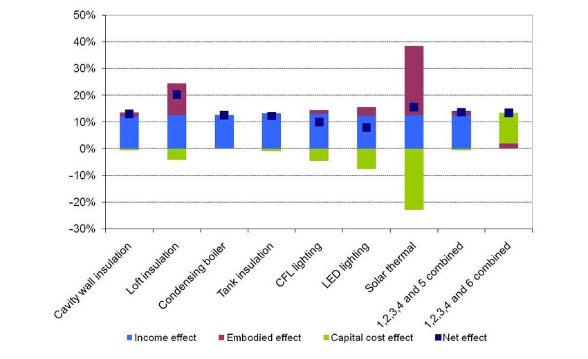
1 Introduction

Global efforts to reduce greenhouse gas (GHG) emissions rely heavily upon improving

energy efficiency in all sectors of the economy. For example, the ambitious ‘450 scenario’,

published by the International Energy Agency (IEA) anticipates energy efficiency delivering

as much as 71% of the global reduction in carbon dioxide emissions in the period to 2020,

and 48% in the period to 2035 (IEA, 2010). The technical and economic opportunities to

improve energy efficiency are particularly large in the built environment which is

consequently the target of multiple policy interventions. But the energy and GHG savings

from such improvements may frequently be less than simple engineering estimates suggest as

a consequence of various rebound effects. If these effects are significant, scenarios that ignore

them are likely to be flawed and to provide misleading guidance for policymakers. But

despite a growing body of evidence on the nature and importance of rebound effects (Sorrell,

2007), they continue to be overlooked by the majority of governments, as well as by

international organisations such as the IEA.

This study seeks to estimate the magnitude of rebound effects following a number of energy

efficiency improvements by UK households. We focus upon measures that improve the

efficiency of heating and lighting systems and we estimate rebound effects in terms of their

effect on global greenhouse gas (GHG) emissions. We extend the existing literature by

accurately quantifying both ‘direct’ and ‘indirect’ rebound effects, and by also allowing for

the emissions ‘embodied’ in energy efficiency equipment such as insulation materials.

The following section provides a classification of rebound effects for households and an

overview of the relevant empirical literature. Section 3 summarises our approach, Section 4

                                               3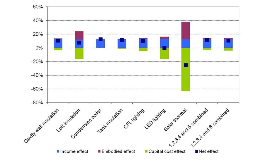
describes the methodology in more detail and Section 5 introduces the analytical tools

employed. Section 6 summarises our specific assumptions and examines their implications

for estimates of rebound effects. Section 0 presents our results and investigates the sensitivity

of those results to selected assumptions. Section 8 concludes.

2 Classifying and estimating rebound effects for
  households
‘Rebound effects’ is an umbrella term for a variety of behavioural responses to improved

energy efficiency. The net result of these effects is typically to increase energy consumption

and carbon/GHG emissions relative to a counterfactual baseline in which these responses do

not occur. As a result, the energy and emissions ‘saved’ by the energy efficiency

improvement may be less than anticipated.

Rebound effects for households have been classified in a number of different ways. To

clarify, we introduce five distinctions.

2.1 Direct versus indirect rebound effects
For households, rebound effects are commonly labelled as either direct or indirect. Direct

rebound effects derive from increased consumption of the, now cheaper, energy services such

as heating, lighting or car travel. For example, the replacement of traditional light-bulbs with

compact fluorescents will make lighting cheaper, so people may choose to use higher levels

of illumination or to not switch lights off in unoccupied rooms. In contrast, indirect rebound

effects derive from increased consumption of other goods and services (e.g. leisure, clothing)

that also require energy and GHG emissions to provide. For example, the cost savings from

more energy efficient lighting may be put towards an overseas holiday. As Figure 1

illustrates, this type of behaviour can be deliberately encouraged!

                                               4
Figure 1 Encouragement of rebound effects
2.2 Energy versus emission rebound effects
Both direct and indirect rebound effects may be estimated in terms of energy consumption,
carbon emissions or GHG emissions, but the magnitude of those effects will differ in each
case. As the average carbon/GHG intensity of energy systems change, the relative magnitude
of these rebound effects will also change – and in some circumstances, rebound effects may
be found to be large in energy terms but small in GHG terms, or vice versa. The estimated
magnitude of energy rebound effects will also depend upon how different energy carriers are
aggregated – for example, on a thermal equivalent basis or weighted by relative prices
(Cleveland et al., 2000).
2.3 Efficiency versus sufficiency rebound effects
Rebound effects do not result solely from cost-effective energy efficiency improvements,
such as purchasing energy-efficient light bulbs, but also from energy-saving behavioural
changes, such turning lights off in unoccupied rooms. These are sometimes referred to as
‘sufficiency’ rather than efficiency actions (Alcott, 2008; Druckman et al., 2011). But while
efficiency improvements will lead to both direct and indirect rebound effects, sufficiency
actions will only lead to indirect effects.
52.4 Direct versus embodied energy use and emissions
Households consume significant amounts of energy ‘directly’ in the form of heating fuels,
electricity and fuels for private cars. But they also consume energy ‘indirectly’, since energy
is used at each stage of the supply chain for all goods and services. For example, energy will
be used to manufacture laptops in China, ship them to the UK and distribute them by road to
retail outlets. This life-cycle energy use is commonly termed embodied energy while the
associated emissions are termed embodied emissions. For OECD households, embodied GHG
emissions frequently exceed the direct emissions associated with consumption of electricity
and fuels. All of these emissions contribute to climate change, but only a portion occur within
national boundaries and hence are covered by national targets on GHG emissions.
While direct rebound effects only affect direct energy use and emissions by the household,
indirect rebound effects affect both direct and embodied energy use and emissions. For
example, the savings from an energy-efficient heating system may be spent upon more
heating (direct rebound, direct emissions), more lighting (indirect rebound, direct emissions)
or more furniture (indirect rebound, embodied emissions).
2.5 Income versus substitution effects
As described in Annex I, both direct and indirect rebound effects may theoretically be
decomposed into income and substitution effects. By making energy services cheaper, energy
efficiency improvements increase the real income of households, thereby permitting
increased consumption of all goods and services and increased ‘utility’ or consumer
satisfaction. These adjustments are termed income effects. But since energy services are now
cheaper relative to other goods and services, households may shift their consumption patterns
even if their real income and hence utility was held constant. These adjustments are termed
substitution effects. The change in consumption for a particular good or service is given by
the sum of income and substitution effects for that good or service. The corresponding
6change in energy use or emissions may be estimated by multiplying the change in
consumption by the energy/emission intensity of that good or service. The direct rebound
effect represents the net result of the income and substitution effects for the relevant energy
service, while the indirect rebound effect represents the net result of income and substitution
effects for all the other goods and services purchased by the household - including other
energy services.
Since the income and substitution effects for any individual good or service may be either
positive or negative, the sum of the two may be either positive or negative. The consumption
of any individual good or service may therefore increase or decrease following the energy
efficiency improvement, and thereby either add to or reduce the household’s aggregate
energy use and GHG emissions.
A stylised example may make this clearer. Suppose a UK household replaces their car with a
more fuel efficient model. Since the fuel costs for driving a given distance are now less, they
may choose to spend some of the money saved on increased leisure driving at weekends
(positive income effect for car travel). Similarly, since the cost of car travel has fallen relative
to the cost of public transport, they may decide to travel to work by car rather than by train
(positive substitution effect for car travel, negative substitution effect for public transport). At
the same time, they may put some of the savings on gasoline expenditures towards a weekend
Eurostar trip to Paris (positive income effect for public transport). The net effect on aggregate
energy use and GHG emissions for the household will depend upon both the change in
consumption of each individual good and service and the energy/GHG intensity of those
goods and services.
72.6 Quantifying direct and indirect rebound effects for households
Table 1 uses the above categories to classify the limited number of studies that estimate both
direct and indirect rebound effects for households. The table also indicates the number of
categories used to classify household goods and services in each study.
The studies listed in Table 1 typically combine estimates of the energy consumption and/or
emissions associated with different categories of household goods and services, with
estimates of how the share of expenditure on these goods and services varies as a function of
prices, income and other variables (Sorrell, 2010). The former are derived from a
combination of Environmentally-Extended Input-Output models and Life Cycle Analysis
(LCA), while the latter are derived from the econometric analysis of survey data on
household expenditure. As indicated in Table 1, existing studies vary widely in the types of
rebound effect covered, the categories used for classifying household expenditures and the
types of actions investigated. While most focus upon improving energy efficiency in
electricity, heating or personal travel, others examine sufficiency actions in those areas, such
as reducing car travel, or broader actions such as reducing food waste. Rebound effects have
been estimated in energy, carbon and GHG terms, but no study estimates and compares all
three. Most studies use income elasticities to simulate the re-spending of cost savings on
different goods and services and consequently capture the income effects of the energy
efficiency improvement but not the substitution effects (for both direct and indirect rebound
effects). While this may appear a drawback, the approach has advantage of being
methodologically straightforward, avoiding the imposition of arbitrary restrictions on
consumer behaviour (e.g. seperability) and allowing the use of relatively high levels of
commodity disaggregation (Sorrell, 2010).
In this study, we estimate the direct and indirect rebound effects following improvements in
the efficiency of heating and lighting systems in UK households. We estimate rebound effects
8in GHG terms and focus solely upon income effects, but extend the existing literature by also
allowing for the emissions embodied in energy efficiency equipment, such as insulation
materials.
9Table 1: Previous estimates of combined direct and indirect rebound effects for households
Author Number of Abatement Area Measure Effects Energy/ Estimated
Commodity action captured emissions rebound effect
Groups (%)
Lenzen and 150 Efficiency and Food; GHGs Income Direct and 45-123%
Day (2002) behavioural heating indirect
change
Alfreddson 300 Behavioural Food; Carbon Income Direct and 7-300%
(2004) change travel; indirect
utilities
Brannlund 13 Efficiency Transport; Carbon Income and Direct and 120-175%
(2007) utilities substitution indirect
Mizobuchi 13 Efficiency Transport; Energy Income and Direct and 12-38%
(2008) utilities substitution indirect
Kratena and 6 Efficiency Transport; Energy Income and Direct only 37-86%
Wuger heating; substitution
(2008) electricity
Druckman 16 Behavioural Transport, GHGs Income Direct and 7-51%et al (2011) change heating, indirect
food
Thomas 74 Efficiency Transport, GHGs Income Direct and 7-25%
(2011) electricity indirect
Murray 36 Efficiency & Transport, GHGs Income Direct and 5–40%
(2011) sufficiency lighting indirect
Note: ‘Effects captured’ refers to the modelling of both direct and indirect rebound effects.
113 Methodology - overview This study focuses upon seven measures that a typical UK household could take to reduce their consumption of electricity or heating fuels, together with their associated greenhouse gas (GHG) emissions (Table 2). Four of these measures represent ‘dedicated’ energy efficiency investments, one represents the ‘natural replacement’ of energy conversion equipment with a more energy efficient option and two represent the ‘premature replacement’ of such equipment.1 In 2009, we estimate that all but one2 of the selected measures were likely to be cost effective for an average UK dwelling, although individual measures are not suitable for all dwellings and the potential cost savings vary widely from one dwelling to another. Between 2008 and 2012, four of the measures were eligible for investment subsidies under the UK Carbon Emissions Reduction Target (CERT). These subsidies are provided by energy suppliers and are funded through a levy on household energy bills, with their availability varying with the socio-economic circumstances of the household (DECC, 2010e).
Table 2: Selected energy efficient measures

No.     Measure                                              Type          Target      Eligible for

                                                                                        subsidy?

1       Cavity wall insulation in un-insulated cavities   Dedicated        Heating         Yes

2       Topping up loft insulation to 270 mm              Dedicated        Heating         Yes

3       Replacing existing boilers with condensing          Natural        Heating         No

        boilers                                           replacement

4       Insulating hot water tanks to best practice (75   Dedicated        Heating         Yes

        mm jacket)

5       Replacing existing incandescent bulbs with        Premature      Electricity       No

        compact fluorescents (CFLs)                       replacement

6       Replacing all existing lighting with LEDs         Premature      Electricity       Yes

                                                          replacement

7       Solar thermal heating                             Dedicated        Heating         Yes

In what follows, we estimate the impact on global GHG emissions of all eligible English

dwellings adopting the relevant measure - for example, installing cavity wall insulation in all

dwellings with unfilled cavity walls. The estimated impacts are the net result of three

different effects which we term as the engineering, embodied and income effects respectively:

     Engineering effect ( ∆ H ): Each measure is expected to reduce the amount of energy

      required to deliver a given level of energy service (e.g. heating, lighting) over its lifetime.

      If consumption of energy services were to remain unchanged, there would be a

      corresponding reduction in household electricity and/or fuel use and the associated GHG

      emissions. Hence, in this paper the engineering effect is an estimate of the change in

      direct GHG emissions for a given energy service assuming that consumption of that

      energy service remains unchanged.

                                                     13
Embodied effect ( ∆M ): The manufacture and installation of the relevant energy efficient
equipment (e.g. insulation materials) is associated with GHG emissions at different stages
of the supply chain. The embodied effect is an estimate of the additional impact on global
GHG emissions of adopting the energy efficiency measure compared to the relevant
alternative. The alternative may be doing nothing in case of dedicated measures,
purchasing less energy efficient equipment in case of natural replacement or continuing to
use existing equipment in case of premature replacement.
Income effect ( ∆ G ): The reduction in the effective price of the energy service is
equivalent to an increase in real household income. This allows households to consume
more goods and services and thereby increase their overall ‘utility’. The income effect is
an estimate of the impact on global GHG emissions of this increased consumption of
goods and services, including energy services. The income effect includes both direct
emissions from the consumption of energy by the household and embodied emissions
from consumption of non-energy goods and services. Emissions from electricity
consumption are commonly labelled as direct, although they occur at the power station.
The estimated total impact ( ∆ Q ) of the energy efficiency measure on global GHG emissions
is given by:
∆ Q = ∆H + ∆ M + ∆G (1)
For each measure, we expect the engineering effect ( ∆ H ) to be negative and the income
effect ( ∆ G ) to be positive. We expect the embodied effect ( ∆ M ) to be positive for
dedicated measures, since the counterfactual involves no investment. But the sign of this
effect is ambiguous for natural and premature replacement measures since the counterfactual
involves investment in inefficient equipment. Overall, we expect each measure to reduce
14global GHG emissions, but by less than simple engineering calculations suggest ( ∆Q ≤ ∆H
). However, if the embodied and income effects exceed the engineering effect, the measure
will increase global GHG emissions (‘backfire’)
The rebound effect (RE) from the energy efficiency improvement may then be defined as:
( Expected savings − Actual savings) ∆H − ∆Q
RE = = (2)
Expected savings ∆H
Or:
∆G + ∆M
RE = − (3)
∆H
This definition (illustrated in Figure 2) treats the embodied effect ( ∆M ) as offsetting some of
the anticipated GHG savings from the measure ( ∆H ) and thereby contributing to the rebound
effect. An alternative approach is to subtract the embodied effect from the anticipated GHG
savings:
∆G
RE * = − (4)
( ∆ H + ∆M )
The difference between the two measures will depend upon the size of the embodied effect
relative to the engineering and income effects.
As defined here, the income effect ( ∆ G ) derives from both increased consumption of energy
by the household (including the energy commodity that benefits from the energy efficiency
improvement) and increased consumption of other goods and services (e.g. clothing,
education). It therefore combines the income component of both the direct and indirect
rebound effect and relates to both direct and embodied emissions. However, it does not
15provide a fully accurate measure of direct and indirect rebound effects because substitution
effects are ignored.
Figure 2 Two definitions of the rebound
r effect
4 Methodology - details
Each measure is assumed to be installed in all eligible dwellings in the UK in 2009 (t=1).
( We
estimate the impact on GHG emissions over a period of T years (t=1 to T)) where T is less
than the economic lifetime of each measure. For simplicity, we present, all our results for a
ten-year period (T=10)
=10) and hold most of the variables affecting GHG emissions fixed over
this period (e.g. household income, commodity prices, number of dwellings etc.). However,
the framework can also allow these variables to change over time. We take 2005 as the
reference year for all real values.
Our approach can be broken down into four stages, as follows.
164.1 Estimating the engineering effect
We use an engineering model (Firth et al., 2009) to estimate the direct energy consumption of
the English dwelling stock by year (t=1 to T) and energy carrier (f). The relevant energy
carriers are gas, oil, solid fuels and electricity. Dividing by the total number of English
dwellings gives the average direct energy consumption per-household ( E ft ). We then apply
the relevant energy efficiency measure to all eligible dwellings (which may be a subset of the
total) and re-estimate the average per-household direct energy consumption ( E' ft ) assuming
the demand for energy services remains unchanged. The change in average annual per-
household direct energy consumption as a result of the measure is then:
∆E ft = E' ft −E ft (5)
These energy savings are assumed to begin in the year of installation of the relevant measure
(t=1). With this approach, the estimated energy savings are averaged over the entire housing
stock but only a portion of dwellings may be eligible for and hence benefiting from the
relevant measure. For example, some dwellings do not have cavity walls while others have
cavity walls that are already filled, so only a proportion of dwellings are suitable for cavity
wall insulation. This means that, in percentage terms, the estimated average energy savings
may be less than would be obtained for an individual dwelling installing the relevant
measure, but they are representative of the potential energy savings obtainable from installing
these measures in the English housing stock as a whole.3
We then use data on the GHG intensity of each energy carrier (sft in kgCO2e/kWh) to estimate
the average per-household change in direct GHG emissions assuming the demand for energy
services remains unchanged. We term this the engineering effect of the energy efficiency
improvement ( ∆Ht ):
17∆H t = ∑ s ft ∆E ft (6)
f
4.2 Estimating the embodied effect
We use the results of a number of life cycle analysis (LCA) studies to estimate the GHG
emissions that are incurred in manufacturing and supplying the relevant energy efficient
equipment and installing it in all eligible dwellings. We assign these embodied emissions to
the year in which the measures are installed and divide by the total number of dwellings to
give the average per-household embodied emissions for the relevant measure ( M 't ). If T is
less than the economic lifetime of the energy efficiency measure, the embodied emissions
will only be relevant for the base year (i.e. M 't = 0 for t>1).
We also estimate the average per-household embodied emissions of the relevant alternative
( M t ). If this alternative has an economic lifetime that is less than T, the measure will avoid
the purchase of conversion equipment in subsequent years, with the result that the embodied
emissions associated with those purchases are also avoided (i.e. Mt > 0 for some t>1). This
is the case, for example, with conventional lighting which has a shorter lifetime than energy
efficient lighting.
The difference between these two estimates represents the incremental embodied emissions
associated with the energy efficiency measure. We term this the embodied effect of the
energy efficiency improvement ( ∆Mt ):
∆Mt = M 't −Mt (7)
184.3 Estimating the income effect
In the UK, household energy bills normally include a fixed annual charge ( a ft in
£/dwelling/year) and a charge per unit of energy used ( k ft in £/kWh). Energy efficiency
improvements only affect the latter. We use data for ‘average’ English dwelling in terms of
energy consumption to estimate the change in average annual energy expenditures following
the adoption of each measure ( ∆Ct ), assuming the demand for energy services remains
unchanged:
∆Ct = ∑ k ft ∆E ft (8)
f
We also estimate the capital cost associated with installing the measure in all eligible
dwellings and divide by the total number of dwellings to give the average per-household
capital cost ( K't ). We do the same for the relevant alternative ( Kt ), with the difference
between the two representing the incremental capital cost of each measure ( ∆K t ):
∆Kt = K 't −Kt (9)
We assume that the full capital costs are incurred in the year in which the measure is installed
(i.e. K 't = 0 for t>1).4 Again, if the relevant alternative has an economic lifetime that is less
than T, the measure avoids equipment purchases in subsequent years (i.e. Kt > 0 for some
t>1). For simplicity, we do not discount these avoided capital costs.
We now look at how these costs affect the average annual real disposable income for a
household (Yt). We treat the sum of the change in energy expenditures and the net capital
payments in a given year as analogous to a change in real disposable income ( ∆Yt ):
19∆Yt = −(∆Ct + ∆Kt ) (10)
Households are assumed to divide their disposable income between their expenditure on
goods and services (Xt) and saving (St). For simplicity, we assume that households save a
fixed fraction (r)5 of their disposable income each year:
∆St = r ∆Yt (11)
We assume that the remainder is entirely distributed between expenditure on different
categories of goods and services – including electricity and fuels. Letting X it represent
expenditure on commodity group i (i=1 to I), then:
I
∆X t = ∑ ∆X it = (1 − r )∆Yt (12)
i =1
From consumer demand theory, this ‘adding up restriction’ leads to the so-called ‘Engel
aggregation condition’, as follows (Deaton and Muelbauer, 1980):
I
∑ βi X it = (1 − r)Yt (13)
i =1
Where βi represents the income elasticity of expenditure for commodity group i:
∆X it Yt
βi = (14)
∆Yt X it
Changes in expenditure on electricity and fuels will lead to changes in direct emissions while
changes in expenditure on other goods and services will lead to changes in embodied
emissions. Savings are treated here as a source of funds for capital investment in the UK
which will also be associated with GHG emissions.6 Hence, changes in expenditure and
20savings in a given year will lead to changes in GHG emissions which may either reinforce or
offset the ‘engineering’ savings in GHG emissions. Letting uit represent the GHG intensity
of expenditure in category i and ust represent the GHG intensity of UK investment7 (both in
kgCO2e/£), the average per-household change in GHG emissions as a consequence of the
change in real disposable income is given by:
I
∆ Gt = ∑ [uit ∆X it ] + u st r∆Yt (15)
i =1
Using Equation 14, the change in expenditure for each category (i) in year t can be written as:
∆Yt
∆X it = βi X it (16)
Yt
Substituting ∆Xit from Equation 16 into Equation 15:
∆Y I
Yt i =1
∑
∆Gt = t [uit βi X it ] + ust r∆Yt (17)
Substituting for Yt from Equation 13, this can also be written as:
I
(1 − rt ) [uit βi X it ] + ust r
∆Gt = ∆Yt I ∑ (18)
i =1
∑
βi X it i =1
We term ∆Gt the income effect of the energy efficiency improvement.
214.4 Estimating the rebound effect
Combining Equations 3 and 18, the rebound effect averaged over a period of T can then be
estimated from:
(1 − rt )
T I
∑ ∆Yt I ∑ [uit βi X it ] + ust r + ∆M t
t =1 βX
∑ i it
i =1
RE = − i =1 (19)
T
∑ ∆Ht
t =1
5 Analytical tools
To develop the above estimates, we combine results from three separate analytical models.
The Community Domestic Energy Model (CDEM) is used to estimate the energy savings
from applying a number of standard energy efficiency measures to UK dwellings; the
Econometric Lifestyle Environmental Scenario Analysis (ELESA) model is used to estimate
how these cost savings are spent on different categories of household goods and services; and
the Surrey Environmental Lifestyle Mapping Framework (SELMA) is used to estimate the
global GHG emissions from the production, distribution and consumption of those categories
of goods and services, together with household savings. These three models are briefly
described below.
5.1 Community Domestic Energy Model (CDEM)
The CDEM model has been developed by Firth et al (2009) at Loughborough University to
simulate energy use in the English housing stock and to explore options for reducing CO2
emissions. The CDEM is one of a family of bottom-up, engineering models of the English
housing stock that are based upon algorithms originally developed by the UK Building
22Research Establishment (Kavgic et al.; Shorrock and Dunster, 1997). The CDEM consists of
two main components: a ‘house archetype calculation engine’ and a core ‘building energy
model’. The archetype calculation engine defines the characteristics of 47 individual house
archetypes, which are used to represent all the dwelling types in the English housing stock.8
The archetypes are defined by different combinations of built form and age (Table 3), since
these variables have a dominant influence on heat loss and hence the energy use for space
heating - the former via average floor area and the number of exposed walls and the latter by
the thermal standards of construction.
Table 3: House archetype categories in the Community Domestic Energy Model
Built form categories Dwelling age band categories
End terrace
Mid-terrace pre-1850; 1851-1899; 1900-1918; 1919-1944; 1945-1964;
Semi-detached 1965-1974; 1975-1980; 1980-1990; 1991-2001
Detached
Flat: purpose-built 1900-1980; 1919-1944; 1945-1964; 1965-1974; 1975-1980;
1980-1990; 1991-2001
Flat: converted or other pre-1850; 1851-1899; 1900-1918; 1990-1944
Note: Pre-1900 purpose-built flats and post-1945 other flats were not considered as these combinations occur very
infrequently in the housing stock.
Model input parameters are defined for each archetype, related to location, geometry,
construction, services and occupancy. The model then estimates the solar gains, internal heat
gains and dwelling heat loss coefficient9 for each archetype and calculates energy
consumption by energy type (solid, gas, liquid and electricity) and end-use (space heating,
hot water, cooking, lights and appliances) under specified weather conditions. Estimates of
the energy consumption in an average dwelling in a given year (Eft) can then be derived from:
23∑ [Nat E fat ]
E ft = at (20)
∑ Nat
a
Where Efat represents the estimated consumption of energy carrier f in archetype a in year t,
and Nat represents the estimated number of dwellings of that archetype in the English housing
stock in that year. We take these estimates, which refer to an average English dwelling, as
representative of the energy consumption of an average UK dwelling.
5.2 Econometric Lifestyle Environmental Scenario Analysis model
(ELESA)
ELESA is a Structural Time Series Model (STSM) (Harvey, 1989) for UK household
expenditure developed by Chitnis et al (2012; 2009) at the University of Surrey. It is
estimated from quarterly time series data on aggregate UK household consumption
expenditure over the period 1964-2009. The model estimates the expenditure on 16 different
categories of goods and services (Table 4) as a function of household income, prices,
temperature (where relevant) and a stochastic (rather than a deterministic) time trend (Hunt
and Ninomiya, 2003). The stochastic trend aims to capture the aggregate effect of underlying
factors such as technical progress, changes in consumer preferences, socio-demographic
factors and changing lifestyles which are difficult to measure (Chitnis and Hunt, 2009;
Chitnis and Hunt, 2010a, b). ELESA is used to forecast future household expenditure and
associated GHG emissions under different assumptions for the relevant variables.
In this study, estimates of the long-run income elasticity ( β i ) for each category are obtained
from ELESA and used within Equation 18 to estimate the income effect.10 These elasticities,
together with household expenditure are held fixed over the projection interval.
24Table 4: Commodity categories
Category (i) CCOIP category Description
1 1 Food & non-alcoholic beverages
2 2 Alcoholic beverages, tobacco, narcotics
3 3 Clothing & footwear
4 4.5.1 Electricity
5 4.5.2 Gas
6 4.5.3 and 4.5.4 Other fuels
7 4.1 to 4.4 Other housing
8 5 Furnishings, household equipment & household maintenance
9 6 Health
10 7.2.2.2 Vehicle fuels and lubricants
11 Rest of 7 Other transport
12 8 Communication
13 9 Recreation & culture
14 10 Education
15 11 Restaurants & hotels
16 12 Miscellaneous goods & services
Notes: COICOP - Classification of Individual Consumption According to Purpose. ‘Other housing’ includes
rent, mortgage payments, maintenance, repair and water supply. Other transport includes non-fuel expenditure
on private vehicles.
5.3 Surrey Environmental Lifestyle Mapping framework (SELMA)
The SELMA model has been developed by Druckman et al (2008) at the University of Surrey
to estimate the GHG emissions that arise in the production, distribution, consumption and
disposal of goods and services purchased in the UK.11 This is known as emissions accounting
from the ‘consumption perspective’ (Druckman et al., 2008; Druckman and Jackson, 2009a,
25c, d; Minx et al., 2009; Wiedmann et al., 2007; Wiedmann et al., 2006). The estimates include
emissions from direct energy use, such as for personal transportation and space heating, as
well as embodied emissions12 from the production and distribution of goods and services. An
important feature of SELMA is that it takes account of all emissions incurred as a result of
final consumption, whether they occur in the UK or abroad. To do this, the estimation of the
embodied emissions is carried out using a Quasi-Multi Regional Environmentally-Extended
Input-Output sub-model (Druckman and Jackson, 2008).
For this study, emissions due to household expenditure are classified into 16 categories
(Table 4) following the rationale outlined in Druckman and Jackson (2009b). The GHG
intensity of expenditure (in kgCO2e/£) in each of these categories ( uit ) is derived by dividing
the estimated GHG emissions associated with UK consumption of those goods and services
by the real expenditure of UK households on those goods and services. Both the emissions
and real expenditure data refer to 2004. We also use the GHG intensity of UK investment in
2004 as a proxy for the GHG intensity of household savings. These estimated GHG
intensities are then held fixed over the projection interval.
6 Assumptions and estimated effects
In this section, we summarise our underlying assumptions and resulting estimates for the
engineering effect ( ∆ H t ), embodied effect ( ∆ M t ) and income effect ( ∆Gt ) respectively. The
estimates are presented for each measure individually, as well as for two combinations of
measures and are averaged over a period of ten years (T=10). The estimates relate to an
‘average’ dwelling, although only a portion of dwellings may be eligible for and hence
benefiting from the relevant measure.
26Some relevant assumptions from the CDEM are summarised in Table 5, while the associated
assumptions for the GHG intensity of delivered energy (in kgCO2e/kWh) and the standing
and unit cost of the energy carriers are given in Table 6. Note that we assume a constant
proportion of low energy lighting and a constant thickness of tank insulation (29.4mm) across
all dwellings, although in practice many dwellings do not have hot water tanks and the
proportion of low-energy lighting varies widely.
Table 5: Some relevant assumptions from the CDM model for 2009
Total number of English dwellings 21,262,825
Proportion of dwellings eligible for cavity wall insulation 39.4%
Proportion of dwellings eligible for topping up loft insulation 67.9%
Proportion of dwellings eligible for condensing boilers 80%
Proportion of dwellings eligible for CFLs, LEDs and tank insulation 100%
Mean net wall area of dwellings eligible for cavity wall insulation 67.3 m2
Mean roof floor area of dwellings eligible for loft insulation 45 m2
Mean thickness of existing loft insulation in dwellings eligible for loft insulation 149 mm
Proportion of households with non-condensing boilers 80%
Mean thickness of existing hot water tank insulation 29.4 mm
Proportion of current light bulb stock that are compact fluorescents 40%
Average number of light fittings per-house 24
27Table 6: GHG intensity and cost of energy carriers for an average UK household in 2009
GHG intensity Standing costs Unit costs
(kgCO2e/kWh) (£/year) (£/kWh)
Gas 0.22554 £93.92 £0.03
Oil 0.30786 - £0.05
Solid 0.41342 - £0.04
Electricity 0.61707 £44.51 £0.11
Sources: (Coals2U, 2011; DECC, 2010a, b; Hansard, 2011)
Notes:
• Nominal costs for a UK household with ‘average’ energy consumption. Costs for gas and electricity
represent a weighted average of credit, direct debit and prepayment customers.
As indicated in Table 7, we estimate that an average English household consumed
approximately 22.5MWh of electricity and fuels in 2009 at a total cost of ~£1100, of which
90% was consumption related (unit costs) and the remainder standing charges. This energy
consumption was associated with approximately 7.1 tonnes of direct GHG emissions.
Electricity accounted for 20% of direct energy consumption, 39% of energy-related GHG
emissions and 45% of energy expenditures. Gas provided the dominant fuel for space and
water heating, accounting for 90% of total fuel consumption and 72% of total energy
consumption. Solid fuels provided a small and declining contribution, accounting for only 4%
of energy use in 2009 and 5% of GHG emissions. We take these estimates as representative
of UK households as a whole.
28Table 7: Estimated annual energy consumption, energy expenditure and energy-related GHG
emissions for an ‘average’ UK dwelling in 2009
Total Total
Gas Electricity Oil Solid fuel energy
Consumption (kWh) 16237 4415 1101 787 18125 22540
Expenditure (£) 509 499 58 32 600 1099
GHG emissions (kgCO2e) 3662 2724 339 325 4326 7051
Note: Expenditures in nominal terms. Total fuel is the sum of gas, oil and solids. Total energy is total fuel plus
electricity.
Estimates of the percentage annual energy ( ∆ E ), cost ( ∆ C ) and GHG ( ∆ H ) savings from
applying the measures all eligible dwellings are shown in Table 8. This also shows the
estimated total impact of applying measures 1, 2, 3, 4 and 5 in combination, as well as
measures 1, 2, 3, 4 and 6 in combination. Since the CDEM cannot be used to simulate solar
thermal heating, we use a variety of sources to estimate the potential energy savings from
fitting solar thermal panels to the estimated 40% of UK households with south facing roofs
(see Annex 2). The results suggest that cavity wall insulation and upgrading to condensing
boilers could each reduce energy-related GHG emissions by ~6%, installing solar thermal
could reduce emissions by ~2.6%, and each of the remaining measures could reduce
emissions by ~1.5%. In combination, the measures have the potential to reduce energy-
related GHG emissions by ~16%, which corresponds to ~5% of total UK GHG emissions and
~4% of the ‘GHG footprint’ (i.e. total direct and embodied emissions) of an average UK
household.13
Since energy-efficient lighting converts less of the input energy into unwanted heat, the
energy and emission savings from this measure may be offset by increased consumption of
29heating fuels in order to maintain internal temperatures (the ‘heat replacement effect’).
Holding demand for energy services constant, we estimate that replacement of existing
lighting by CFLs and LEDs will increase total household energy consumption by ~1%, but
reduce energy costs by ~5% and energy-related GHG emissions by ~1.3%. Similarly, our
estimates account for the reduction in the marginal energy savings from individual measures
when used in combination with others.
Table 8: Estimated annual savings in energy consumption, energy costs and energy-related
GHG emissions from applying the measures to an ‘average’ UK dwelling in 2009
No. Measure Annual Annual Annual GHG Ratio
energy saving energy cost saving (%) of cost
(%) saving (%) to
GHG
savings
1 Cavity wall
insulation 7.3 4.9 5.9 0.83
2 Loft insulation 1.9 1.3 1.5 0.87
3 Condensing boiler 8.4 4.7 5.9 0.79
4 Tank insulation 1.7 1.5 1.7 0.88
5 CFLs 0.1 1.4 1.2 1.16
6 LEDs 0.2 1.7 1.4 1.22
7 Solar thermal 3.1 2.6 2.5 1.04
8 1,2,3,4 and 5 18.5 13.2 15.6 0.85
9 1,2,3,4 and 6 18.5 13.5 15.8 0.85
30Annex 3 summarises our assumptions and estimates for the embodied effect of each measure
( ∆ M ). These are based upon LCA studies for the relevant materials and equipment, but this
evidence is patchy and frequently makes inconsistent assumptions for key variables such as
the GHG intensity of electricity. We assume that the incremental embodied emissions
associated with the natural replacement of existing boilers are zero and we provide two sets
of estimates for energy efficient lighting - the first allowing for the EU phase-out of
incandescent bulbs in the period to 2016 and the second assuming that these bulbs continue to
be available. In the latter case, installing energy efficient lighting allows consumers to avoid
replacing incandescent bulbs at two-year intervals over the subsequent ten years (see Annex
1). Since the embodied emissions associated with these purchases are also avoided, the
second scenario leads to a lower estimate of the incremental embodied emissions associated
with energy efficient lighting.
Table 9 summarises our estimates for the incremental capital cost of each measure ( ∆ K )
which are based upon information provided by the UK government (DECC, 2010d). Several
of the measures are eligible for subsidies through CERT, with the level of subsidy being
greater if the head of the house is at least 70 years old or is in receipt of certain income-
related benefits. Approximately 11.2 million UK households (42%) fall into this so-called
Priority Group (PG), and DECC (2010d) estimates that approximately 55% of CERT-
subsidised measures will be installed in PG households. Hence, the estimates take into
account both the level of subsidies available for PG and non-PG households and the relative
proportion of installations expected within each. As with the embodied effect, we assume that
the incremental capital cost of replacing an existing boiler with a condensing boiler is zero
and we provide two sets of estimates for energy efficient lighting.
31Table 9: Estimated incremental capital cost for an ‘average’ UK dwelling over a period of
ten years
No. Measure Incremental capital cost – no Incremental capital cost -
subsidy with subsidy
(£) (£)
1 Cavity wall insulation 179 41
2 Loft insulation 235 54
3 Condensing boiler - -
4 Tank insulation 17.50 6.3
5 CFLs 57.6 (-21.6) 57.6 (-21.6)
6 LEDs 254.4 (175.2) 127.2 (48)
7 Solar thermal 1489 532
8 1,2,3,4 and 5 409.9 79.7
9 1,2,3,4 and 6 256.3 53.3
Note: Estimates refer to an ‘average dwelling’ and are derived by estimating the capital costs associated with
installing the measure in all eligible dwellings and dividing by the total number of dwellings. Estimates in
brackets for energy efficient lighting are without allowing for the EU ban on incandescent bulbs.
Table 10 summarises our assumptions for the expenditure share ( X i / X ), long-run income
elasticity ( β i ), GHG intensity of expenditure ( u i ) and share of total household GHG
emissions for each of the 16 categories of goods and services (see also Figure 3). Expenditure
on domestic energy (i.e. gas, electricity and other fuels) accounted for 2.4% of household
income in 2009, but this figure hides considerable variation between individual households.
Approximately 4 million English households (18.4%) were estimated to be in ‘fuel poverty’
in 2009 - defined as needing to spend more than 10% of their income on energy in order to
maintain an adequate standard of warmth (Hills, 2011).14
32Figure 3 (panel 2) illustrates that the GHG intensity of expenditure ( u i ) on electricity, gas
and other fuels is approximately four times greater than the mean GHG intensity of
expenditure on the other commodity groups and ten times greater than the share-weighted
mean. But this high GHG intensity is offset by the relatively small share of energy in total
expenditure (Figure 3, panel 1), with the result that domestic energy consumption accounts
for less than one quarter of the GHG footprint of an average UK household (~28tCO2e/year)
(Druckman and Jackson, 2010). ‘Other transport’ accounts for around 16% of the total GHG
footprint (Figure 3, panel 3), owing to the large contribution from aviation fuels, together
with the emissions that are embodied in private cars and associated infrastructure. Aviation is
estimated to account for ~5% of the total GHG emissions of an average UK household,
despite the fact that up to half of UK households do not fly in an average year (Cairns et al.,
2006). Moreover, allowing for the additional radiative forcing from contrails and nitrogen
oxides could double this figure (Druckman and Jackson, 2010; RCEP, 2007). For car travel,
the embodied emissions in vehicles and other infrastructure are only slightly less than the
direct emissions from vehicle fuels which account for 9% of an average household's footprint
(Figure 3, panel 3).
33Table 10: Estimated expenditure shares, income elasticities and GHG intensities
No. Description Real Long-run GHG GHG GHG
expenditure income intensity intensity emissions
share in elasticity (kgCO2e/ as % of as % of
2009 (%) £) gas total
( Xi / X ) ( βi ) ( uit )
1 Food & non-alcoholic 0.18 1.3
beverages 7.9 14.0 11.7
2 Alcohol and tobacco 3.2 0.29 0.2 2.2 0.7
3 Clothing & footwear 6.6 0.36 0.4 4.3 3.0
4 Electricity 1.1 0.30 8.0 78.5 9.1
5 Gas 1.2 0.00 9.3 100.0 12.4
6 Other fuels 0.1 0.35 10.3 110.8 1.6
7 Other housing 15.8 0.15 0.3 3.2 5.4
9 Furnishings etc. 4.7 0.70 0.7 7.5 3.7
9 Health 1.7 0.08 0.3 3.2 0.6
10 Vehicle fuels and lubricants 2.9 0.08 2.8 30.1 9.2
11 Other transport 10.7 0.50 1.3 14.0 15.8
12 Communication 2.1 0.17 0.3 3.2 0.7
13 Recreation & culture 12.5 0.37 0.5 5.4 7.1
14 Education 1.2 -0.23 0.3 3.2 0.4
15 Restaurants & hotels 8.6 0.68 0.6 6.5 5.9
16 Miscellaneous 12.5 0.41 0.5 5.4 7.1
Saving 7.8 0.0 0.6 6.5 5.3
Source: GHG intensity estimates from SELMA. Elasticity estimates from ELESA. Expenditure share estimates
from the UK Office of National Statistics (ONS).
34by commodity group
Figure 3 Expenditure shares, GHG intensities and share of total household GHG emissions
GHG intensity (kgCO2e/£) Expenditure share (%)
10
12
14
16
18
0
2
4
6
8
10
12
0
2
4
6
8
Food & non-…
Alcohol and tobacco
Clothing & footwear
Electricity
Gas
Other fuels
Other housing
35
Furnishings etc.
Health
Vehicle fuels and…
Other transport
Communication
Recreation & culture
Education
Restaurants & hotels
Miscellaneous
SavingsShare of GHG emissions (%)
10
12
14
16
18
0
2
4
6
8
36Table 11 and Figure 4 summarise the resulting estimates for the engineering ( ∆ H ),
embodied ( ∆ M ) and income ( ∆ G ) effects for each of the measures, averaged over a ten
year period. This demonstrates that, averaged across all measures, the embodied effect is
around 40% of the income effect (or 15% if solar thermal is excluded), while the income
effect is around 13% of the engineering effect. The implications of this for the estimated
rebound effects (RE) are explored below.
The estimated contribution of each commodity group to the income effect (Figure 5) depends
upon the product of its expenditure ( X i ), GHG intensity of expenditure ( u i ),and income
elasticity ( β i ). So for example, vehicle fuels are GHG intensive, but only account for 2.5% of
the estimated income effect owing to their small share of total expenditure (2.1%) and low
income elasticity (0.08). In contrast, other transport is only one third as GHG intensive as
vehicle fuels, but accounts for 26% of the estimated income effect owing to its large
expenditure share (11.5%), and high income elasticity (0.5). This suggests that our results
could be sensitive to the elasticity estimates used – and in particular to our estimate of a zero
income elasticity for gas.15 We test the sensitivity of our results to this elasticity below.
37Table 11: Estimated engineering, embodied and income effect from each measure for an
‘average’ dwelling over a ten year period (percentage of baseline GHG emissions)
No. Measure Engineering effect Embodied effect Income effect
( ∆H ) ( ∆M ) ( ∆G )
1 Cavity wall insulation -8.8 0.13 1.10
2 Loft insulation -2.3 0.27 0.29
3 Condensing boiler -9.0 0.00 1.16
4 Tank insulation -2.6 0.01 0.33
5 CFLs -2.1 0.03 0.28
6 LEDs -2.5 0.08 0.33
7 Solar thermal -3.8 0.99 0.48
8 1,2,3,4 and 5 -23.8 0.41 3.01
9 1,2,3,4 and 6 -24.2 0.46 3.07
Note: Estimates refer to an ‘average dwelling’ and are derived by estimating the total effect associated with
installing the measure in all eligible dwellings and dividing by the total number of dwellings.
Figure 4 Estimated engineering, embodied and income effect from each measure for an
‘average’ dwelling over a ten year period (%)
5.00%
0.00%
Change in GHG emissions (%)
-5.00%
-10.00%
-15.00%
-20.00%
-25.00%
-30.00%
Engineering effect Embodied effect Income effect
38Figure 5 Estimated contribution of different commodity groups to the income effect
30
Contribution to income effect (%)
25
20
15
10
5
0
-5
7 Results
In this section, we present our estimates of the rebound effects from the different measures
averaged over a period of ten years. We present the results in four stages, namely:
income effects only, ignoring capital costs;
income and embodied effects, ignoring capital costs;
income and embodied effects, allowing for capital costs; and
sensitivity to key variables.
7.1 Income effects only
Figure 6 illustrates the estimated rebound effect from income effects alone, ignoring both the
embodied effect and the capital cost of the measures. This shows that the estimated rebound
effects are modest and broadly comparable across all measures, with a mean of 12.4% for the
heating measures 13.0% for energy efficient lighting and 12.5% for the two combinations of
measures. These estimates are lower than many in the literature and derive from the fact that
39the bulk of the cost savings are spent on commodities that have a significantly lower GHG
intensity than domestic energy consumption. The difference between the estimated rebound
effects for lighting and heating measures is relatively small, implying that both measures save
a comparable amount of money for each kg of GHG saved. This is because, in our model,
expenditure on electricity is ~80% as GHG intensive as expenditure on natural gas. If
rebound effects were to be measured on an energy basis, the difference between the two
measures may be larger.
Figure 6 also breaks down the income effect into direct and embodied emissions- where the
former relates to increased consumption of energy commodities (electricity, gas and other
fuels) and the latter relates to increased consumption of other goods and services. This shows
that embodied emissions are substantially more important than direct emissions - with the
latter accounting for only 13% of the total.
The estimated rebound effect for energy efficient lighting is influenced by our modelling of
the heat replacement effect (i.e. the increased use of heating fuels to compensate for the loss
of heat from incandescent bulbs). Heat replacement reduces the engineering effect from
energy efficient lighting by proportionately more than the income effect. Hence, when there
is no heat replacement, our estimate of the rebound effect for lighting falls to 10% (implying
a ‘heat replacement rebound’ of around 3%).
Our estimates are comparable with those from earlier studies that used a similar methodology
to investigate lighting and heating measures. For example, Druckman et al (2011) estimate a
7% rebound effect following adjustment of thermostats by UK households, Murray (2011)
estimates a 5% rebound effect following electricity conservation measures by Australian
households and Thomas (2011) estimates a 7% rebound effect following improvements in
electricity efficiency by US households.
40Figure 6 Estimated rebound effects from income effects alone, showing contribution of direct
and embodied emissions
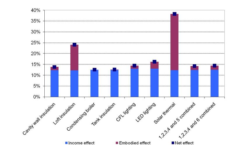
7.2 Allowing for the embodied effect
Figure 7 illustrates how the rebound effect is modified when an allowance is made for the
embodied effect. Ignoring capital costs, this leads to a mean rebound effect of 20% for the
heating measures (or 16% without solar thermal), 15% for the lighting measures
measures and 14% for
the two combinations of measures. The embodied effect is estimated to account for 10% of
the rebound effect for cavity wall insulation, 20% for LED lighting, 49% for loft insulation
and 67% for solar thermal. This demonstrates that the embodied
embodied effect should not be ignored,
but is nevertheless relatively modest for all the measures considered. The exception is solar
thermal, but even this has an estimated ‘GHG payback time’16 of less than three years. The
contribution of the embodied effect
effec to the rebound effect also depends upon the time interval
of interest. For example, averaging over five years raises the estimated rebound effect for the
two combinations of measures by one percent. However, the most appropriate metric is the
41full economic lifetime of the relevant measure which in the case of insulation and solar
thermal is many decades. Over this period, the engineering savings greatly exceed the
embodied emissions of the relevant equipment.
These results treat the embodied effect ( ∆M ) as offsetting some of the anticipated GHG
savings from the measure ( ∆H ) and thereby contributing to the rebound effect. An
alternative approach (Equation 4) is to subtract the embodied effect from the anticipated
GHG savings. This reduces the mean rebound effect to 14% for the heating measures (or 13%
without solar thermal), and to 13% for both the lighting measures and the two combinations
of measures. Once again, this demonstrates that, with the exception of solar thermal, the
income effect dominates.
Figure 7 Estimated rebound effects from income and embodied effects, ignoring capital costs
427.3 Allowing for capital costs
Figure 8 illustrates how allowing for capital costs reduces the net cost saving from each
measure and hence the estimated rebound effect - leading to a mean rebound effect of 3.4%
for the heating measures (or 11% if solar thermal is ignored), 5% for the lighting measures
and 11% for the two combinations of measures. With the assumptions used here, both solar
thermal and LEDs are estimated to have a simple payback that exceeds ten years and hence
are found to have a negative rebound effect over this period. Taking the CERT subsidies into
account (Figure 9) leads to higher net cost saving and hence higher rebound effects –
respectively 15% for the heating measures, 9% for the lighting measures and 14% for the
two combinations of measures.
In practice, only a portion of eligible households will benefit from subsidies and these are
currently funded through higher energy bills for all household consumers (Sorrell et al.,
2009c). For example, DECC (2010c) estimates that CERT raised household gas prices by
2.8% in 2010 and household electricity prices by 3.3%. These energy price increases will
reduce real household incomes and expenditures and hence reduce both energy-related and
total GHG emissions. As a result, the positive income effect from the energy efficiency
improvements will be offset by a negative income effect from the energy price rises - for both
participants and non-participants in CERT (Sorrell et al., 2009c). To properly account for
this, it would be necessary to estimate the proportional contribution of each measure to the
overall increase in energy prices.
These estimates also assume implementation of the EU Directive on energy efficient lighting.
If instead, we assume that incandescent bulbs continued to be available, the embodied effect
of energy efficient lighting would be lower (since the emissions embodied in subsequent
purchases of incandescent bulbs would be avoided), but the income effect would be higher
43You can also read