Generalized Parking Occupancy Analysis Based on Dilated Convolutional Neural Network - MDPI
←
→
Page content transcription
If your browser does not render page correctly, please read the page content below
sensors
Article
Generalized Parking Occupancy Analysis Based on
Dilated Convolutional Neural Network †
Sherzod Nurullayev and Sang-Woong Lee *
 Pattern Recognition and Machine Learning Lab., Gachon University, 1342 Seongnamdaero, Sujeong-gu,
 Seongnam 13120, Gyeonggi-do, Korea; sfreedom9393@gmail.com
 * Correspondence: slee@gachon.ac.kr; Tel.: +82-31-750-6918
 † A preliminary version of this paper has been presented in 4th International Conference on Next Generation
     Computing which was held in Vung tau, Vietnam, 20–23 December 2018.

 Received: 12 November 2018; Accepted: 8 January 2019; Published: 11 January 2019

 Abstract: The importance of vacant parking space detection systems is increasing dramatically as the
 avoidance of traffic congestion and the time-consuming process of searching an empty parking space
 is a crucial problem for drivers in urban centers. However, the existing parking space occupancy
 detection systems are either hardware expensive or not well-generalized for varying images captured
 from different camera views. As a solution, we take advantage of an affordable visual detection
 method that is made possible by the fact that camera monitoring is already available in the majority of
 parking areas. However, the current problem is a challenging vision task because of outdoor lighting
 variation, perspective distortion, occlusions, different camera viewpoints, and the changes due to
 the various seasons of the year. To overcome these obstacles, we propose an approach based on
 Dilated Convolutional Neural Network specifically designed for detecting parking space occupancy
 in a parking lot, given only an image of a single parking spot as input. To evaluate our method
 and allow its comparison with previous strategies, we trained and tested it on well-known publicly
 available datasets, PKLot and CNRPark + EXT. In these datasets, the parking lot images are already
 labeled, and therefore, we did not need to label them manually. The proposed method shows more
 reliability than prior works especially when we test it on a completely different subset of images.
 Considering that in previous studies the performance of the methods was compared with well-known
 architecture—AlexNet, which shows a highly promising achievement, we also assessed our model in
 comparison with AlexNet. Our investigations showed that, in comparison with previous approaches,
 for the task of classifying given parking spaces as vacant or occupied, the proposed approach is more
 robust, stable, and well-generalized for unseen images captured from completely different camera
 viewpoints, which has strong indications that it would generalize effectively to other parking lots.

 Keywords: parking occupancy detection; dilated convolution; PKLot; AlexNet; CarNet

1. Introduction
     The noteworthy growth of the automotive industry together with a lack of urban planning have
caused problems such as traffic congestion, air contamination, and driving difficulties. To facilitate
consumers, most car manufacturers provide a pre-installed or aftermarket navigation system in
vehicles. This enables drivers to easily navigate to their destination. However, navigation systems
provide a rough estimate of the remaining distance to the destination.
     With the recent technological advancements in sensing and intelligent technologies, companies
are interested to find out whether these advancements can assist in reducing the time spent to search
for vacant parking spaces. Locating an unoccupied parking space is a major predicament that drivers
face since searching it is a tedious process. Thus, systems that can detect vacant parking spaces will

Sensors 2019, 19, 277; doi:10.3390/s19020277                                   www.mdpi.com/journal/sensors
Sensors 2019, 19, 277                                                                              2 of 25

enable drivers to efficiently locate vacant parking spaces. Such systems are referred to as, parking
guidance systems (PGSs). PGS can decrease the time consumed by drivers in searching for a parking
space and help them avoid driving impediments. As a subsidiary effect PGSs relieve overall traffic
congestion in city centers, consequently, decrease fuel consumption and CO emissions. The goal of
PGS is to obtain the most credible and definitive data from parking vacancies and provide them in
a form that is most helpful for consumers. PGSs differ considerably in their detection performance,
optimization, and reporting process. Our goal is to improve the detection performance of a PGS. Three
principal factors should be considered when selecting a detection scheme. Robustness is the primary
factor. A robust indicator should accurately provide the status of a parking space, despite the diversity
in environmental parameters, such as temperature, and the varieties of cars and parking slots. Second,
maintenance is an additional determinant that must be considered, together with the cost of new tools
to be purchased per parking stall, the deployment effort, and the necessity to restrict normal parking
throughout the installation period. Third, the number of sensing units clearly has a direct effect on the
establishment and maintenance expenses of a detection system.
      To resolve this problem, researchers have proposed methods can be characterized as counter-,
sensor-, and image-based. Counter-based methods compute the number of cars entering and exiting
the parking section. Thus, systems based on these methods include gate-arm counters and inductive
loop detectors positioned at the gates of parking facilities. The systems’ display panels show reports
and directions and guide the driver toward a vacant parking space. This type of arrangement can
notify the total number of unoccupied spaces; however, it does not guide a driver to the exact location
of a vacant parking space. An alternative approach is to use sensors (such as ultrasonic, inductive
loop, and infrared laser sensors), which can be pre-installed in each parking space for indicating
its occupancy status. These sensors are normally reliable; however, the principal disadvantage of
sensor-based methods is the cost of building the system because a great number of sensor units are
needed to cover the entire parking area. A vision-based detector can overcome the shortcomings of
sensor per-stall and counter-based detection methods. A vision-based system is an optimal choice
since its installation is manageable and it demands no closedowns. Moreover, computer vision for
traffic applications is an emerging area of research, including notable advances in the last few years.
For instance, intelligent transportation management systems, like those investigated in [1], attempt
to achieve tasks such as tracking, detection, and identification of vehicles, as well as higher-level
assignments like comprehending vehicle behaviors and exposing irregularities. In a vision-based
system, every visual node which includes a camera and a transmitter can observe multiple vehicles
concurrently, decreasing the cost per parking stall. As it can be adopted for other tasks, such as
surveillance, the basis of the system is usually already installed, and it can be managed by other
applications after deployment. However, those who advocate sensor-based methods, such as the
authors of [2], claim that video cameras are considerably more expensive than sensors and produce a
large volume of data that may not be easily disseminated through a wireless network. On the contrary,
a review of the literature, [3], revealed that image-based parking reservation detection policies can be
deployed using extant surveillance cameras that are already attached to a primary monitoring system.
Thus, it appears that image-based systems are a valid choice, especially for very large or outdoor
parking areas where the installation of hundreds of sensors is impracticable. In consideration of this,
many vision-based parking space management systems have been discussed and developed recently.
Frequently, researchers turn to solve the issue with deep learning since it can extract features and
learn to classify automatically. Deep networks, such as convolutional neural networks (CNNs), are
robust to lighting variations and diverse circumstances. Nevertheless, without adjustment, a standard
CNN cannot operate for all possible conditions. Thus, to create a robust parking space location
system, we should take many difficulties into account, such as lighting variations, varying vehicle
sizes, illuminance, perspective distortion, inter-object occlusion, camera resolution, and unfavorable
weather. Most previous efforts were focused on resolving these difficulties. However, this task cannot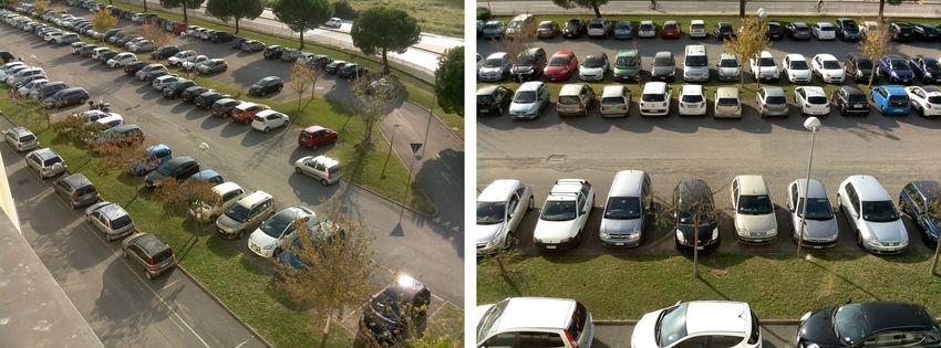
Sensors 2019, 19, 277                                                                              3 of 25

be simply generalized and indeed the adaptation of a specific solution to an unknown parking lot is
not easy.
     In this paper, to address the aforementioned issues, we introduce a CNN structure that uses dilated
convolutional neural networks to indicate parking space occupancy status. The PKLot dataset [4],
which is publicly accessible, was used to evaluate the performance of our model. The use of images of
different scenarios and parking areas allowed us to test the generalizability of our approach. We trained
our model on one subset of images and tested it on a completely different one. Several approaches
already exist, such as that investigated in the study reported in [5], mAlexNet, where this type of
generalization property was tested experimentally; however, we show that our method outperforms
them. Most of the related studies compared their approach with AlexNet [6], which has demonstrated
a high-level performance on this task. Thus, we analyzed our approach in comparison with AlexNet,
as well as with other well-known deep learning structures.
     The remainder of the paper is organized as follows. Section 2 reviews the related work. The features
of the dataset we used in our experiments are described in Section 3. In Section 4, we provide a detailed
explanation of our classification method. Our experiments and the obtained results are described in
Section 5. Finally, Section 6 concludes the paper.

2. Related Work
     To overcome the problem described above, there currently exist various systems, such as those
proposed in [2,7–23]. In some studies, the parking management system problem was addressed
by using smart devices [24–27]. Sensor-based systems involve detection sensors, such as ultrasonic
sensors, which are installed at each parking space [11,28–30]. Huang and Wang [31], stated that
image-based methods can be categorized into two classes: space-driven and car-driven. Space-driven
methods are focused on identifying vacant parking places rather than cars [8,32]. For images obtained
from static (such as the surveillance) cameras, the strategy most frequently applied is background
subtraction [33], which assumes that the variation in the background is statistically motionless within
a small interval of time. Considering this assumption does not hold for outdoor scenes, the limits of
this approach are immediately clear. A more robust method was proposed in [34]. The authors used
Gabor filters to train a classifier with images of unoccupied parking spaces under various lighting
conditions. In the car-driven method category, algorithms are trained to recognize automobiles, which
are the objects of interest. Related to this issue are a few object detection methods that were proposed
in [35,36]. Because of the perspective distortion observed in most images of parking lots, such as that
shown in Figure 1, cars located at a considerable distance from the camera occupy a small area in an
image, and thus, fewer details can be observed, which considerably diminishes the performance of
object detection algorithms. The method introduced in [5], is based on a deep Convolutional Neural
Network specifically designed for smart cameras. They achieved fairly high results and we will
be comparing our results with respect to it. The method, called mAlexNet, is a version of AlexNet
and offers a decentralized solution for visual parking space occupancy detection. It achieved very
good results, but only for the same subset of images. In [37], the problem of occlusion of parking
spaces, where one or more parking spaces can be hidden by other parked vehicles, was addressed.
To solve the occlusion problem, vehicle tracking to detect the events of a car entering or exiting a
parking space has been suggested. Furthermore, in addition to methods that use visual techniques and
ground sensors, methods exist that use sensors installed on cars or carried by drivers. For instance,
in [38], a framework for detecting parking space occupancy in which the system collaborated with
in-vehicle navigation systems was proposed. In [39], a crowd-sourcing solution, leveraging sensors
in smartphones, was proposed for collecting real-time parking availability data. In the context of
vehicle detection, the single method of which we have knowledge that uses a CNN is that presented
in [40]. It uses a multi-scale CNN to detect vehicles in high-resolution satellite images. In addition
to providing a dataset, the authors of [4], addressed the problem by applying machine learning
techniques. They used their dataset, which contains approximately 700,000 images of parking spaces in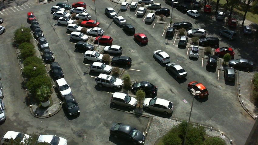
Sensors 2019, 19, 277                                                                             4 of 25

parking lots captured by three different cameras, to train SVM classifiers on various textural features,
such as LBP, LPQ, and their variations. They additionally enhanced the detection performance by
using composites of SVMs, applying simple aggregation functions, such as maximum or average,
to the confidence values given by the classifiers. We will be comparing our work with respect to
it. In the method presented in [41], specifically trained customized neural networks were used to
ascertain parking space occupancy statuses and parking demand based on visual features extracted
from images of parking spaces. The method’s performance evaluation, conducted in a 24-h period
and based on 126 parking spaces, showed that the classifier yielded promising results for night and
day. The authors of [42], used a Bayesian hierarchical structure to formulate a vacant parking space
detection scheme, which is based on a 3D model for parking spaces, that can operate day and night.
Likewise, the design presented in [43], models every parking space as a volume in 3D space and is
thus able to consider occlusions when estimating the probability that a vehicle is present in a parking
space. In [44], the authors attempted to remove the occlusion problem from which the former approach
suffers by classifying the state of three bordering spaces as a unit and using a color histogram of
the three spaces as the feature for their SVM classifier. To handle the problem of lighting changes,
in the study [45], a Bayesian classifier based on corners, edges, and wavelet features was applied
to verify the detection of vehicles. Moreover, in [46], methods that use aerial images for detecting
vacant parking spaces were presented. The authors proposed a self-supervised learning algorithm
that automatically obtains a set of canonical parking space templates to learn the appearance of a
parking space and estimates its structure from the learned model. In [47], LUV color space, gradient
magnitude and six quantized gradient channels are used as features and feed into machine learning
methods, Linear Regression and SVM to detect the status of a given parking place. Since the results
they achieved are high, we will be comparing our work with respect to it. The limitation of this method
is its relatively low detection accuracy.

                        Figure 1. Example for a car parking area taken from PKLot dataset [4].

3. Datasets

3.1. PKLot Dataset
     By reason of the vast number of possible applications, parking lot status detection schemes have
attracted a great deal of research attention in the last decade. However, in the computer vision field,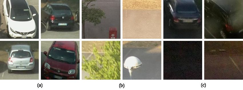
Sensors 2019, 19, 277                                                                                       5 of 25

the lack of datasets that can be used to assess and analyze proposed algorithms is a problem that
researchers face frequently. An example of a parking area is shown in Figure 1.
      To overcome this difficulty, as mentioned above the contributors of [4], introduced the PKLot
dataset, which offers an important resource for researchers and practitioners whose objective is to create
outdoor parking space vacancy detection systems. As our goal is to classify parking space occupancy,
the PKLot dataset is one of the most appropriate candidate resources for facilitating this task, providing
images captured in two parking lots from three separate camera views. It succeeds in solving the
problem regarding the lack of a common dataset, allowing future benchmarking and evaluation. This
dataset contains images captured on sunny, rainy, and overcast days, and thus, we found it a very
useful tool for our research purpose. The PKLot dataset contains 12,417 images of parking areas and
695,899 images of parking spaces segmented from them, which have been manually checked and
labeled. All the images were captured in the parking areas of the Federal University of Parana (UFPR)
and the Pontifical Catholic University of Parana (PUCPR), both located in Curitiba, Brazil. The cameras
were located on the roof of the buildings to decrease the potential occlusion of adjacent cars. Moreover,
such settings allow series of pictures that vary widely in terms of changing illumination caused by
weather variations to be obtained. To build a more challenging dataset, in [4], images presenting
difficulties, such as images of vehicles that are overexposed because of sunny conditions, images with
shadows caused by trees, and images collected during heavy rain that resemble pictures captured
at night because of the lack of natural light, were included in the dataset. An essential detail of this
dataset is that only legal parking spaces were marked and segmented. The parking lots those are
signed (delimited) with parallel yellow or white lines on the floor are considered as legal ones. As one
may remark, there might be some automobiles parked in an illegal manner like in the middle of the
street. The pictures were saved in JPEG color format with lossless compression in a resolution of
1280 × 720 pixels. The pictures taken from the cameras were cropped by the authors of [4], into single
parking space images, rotated and grouped. Some of the examples of occupied and vacant parking
spaces are shown in Figure 2.

      Figure 2. (a) example of a parking lot in PKLot dataset [4]; (b) example images of empty parking spaces
      after cropping and rotating; (c) example images of occupied parking spaces after cropping and rotating.

    All the cropped images were arranged into three subsets by the authors of [4] and named as
UFPR04, UFPR05, and PUCPR. The first two subsets contain pictures of varied views of the same
parking area captured from cameras located on the 4th and 5th floors of the UFPR building. Images
captured from the 10th floor of the administration building of PUCPR constitute the third subset.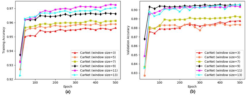
Sensors 2019, 19, 277 6 of 25
Our investigations showed that UFPR04 is a more challenging subset than UFPR05 and PUCPR
because it contains images with diverse obstacles and ground patterns. The subset contains 3791
images captured under the aforementioned weather conditions. To these images, a semi-automatic
segmentation process was applied and they were also manually labeled. A total of 105,845 images of
individual parking spaces, 43.48% occupied and 56.42% vacant, was generated during the process.
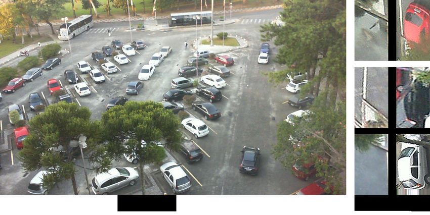
A very similar report was produced for the PUCPR and UFPR05 subsets. In [4], all three subsets,
PUCPR, UFPR04, and UFPR05, were categorized manually into overcast, sunny, or rainy subfolders
according to the observed weather conditions. Figure 3 shows some example images of the three
parking areas obtained under the before-mentioned weather conditions.
Figure 3. Examples of photos taken under various weather conditions [4]: (a–c) from PUCPR (sunny,
overcast, rainy respectively); (d–f) from UFPR04 (sunny, overcast, rainy respectively); (g–i) from
UFPR05 (sunny, overcast, rainy respectively).
The available images show a wide luminance variation because they were captured under different
climatic conditions. They were used for examining the performance of classifiers trained on images of
a single parking lot. A brief review of the factors that distinguish this dataset and render it useful is
as follows:
• The captured images show various parking areas having dissimilar features.
• Generally, commercial surveillance system cameras are placed at a high above the cars,
and therefore, they can observe all the vehicles in a certain parking place. However, this makes
our task more challenging, and therefore, the cameras were positioned at various heights to obtain
a variety of images.
• The images were captured under diverse weather conditions, such as sunny, rainy, and overcast,
which represent various illumination conditions.
• Various types of challenges, such as over-exposure due to sunlight, differences in perspective,
the presence of shadows, and reduced light on rainy days, are provided by the current
dataset images.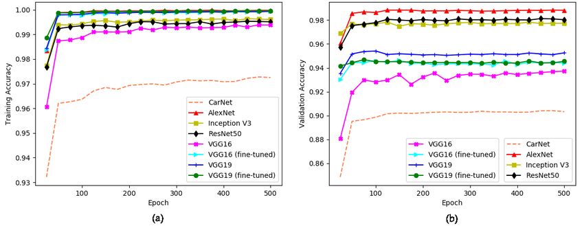
Sensors 2019, 19, 277                                                                                  7 of 25

3.2. CNRPark + EXT Dataset
     The dataset provides a great facility to researches containing nearly 150,000 labeled pictures
of empty and used parking spaces. A smaller dataset of approximately 12.000 designated images,
CNRPark [21], is covered and noticeably enlarged by CNRPark + EXT, reference [5]. Reference [21]
holds parking lot pictures obtained in various days of July 2015, from 2 different cameras A and B,
which were installed in order to have diverse viewpoints.
     Similarly, CNRPark dataset is also publicly accessible. The CNRPark + EXT is a significant
expansion of CNRPark dataset with images obtained from November 2015 to February 2016 under
different weather circumstances by 9 cameras with distinct angles of view. Examples are given by
Figure 4.

                          Figure 4. Example photos from CNRPark + EXT dataset [5].

     Partial occlusion patterns due to obstructions such as lampposts, trees, other cars, and different
lighting conditions are involved in this dataset. See Figure 5. This enables training a classifier that is
able to characterize most of the challenging circumstances that can be detected in a real-life scenario.
Similar like PKLot dataset, CNRPark dataset also provides cropped images from pictures taken by
cameras making our work easier. Each image represents a single vacant or occupied parking space.
Examples of these patches are given in Figure 5.

      Figure 5. Parking spaces (patches) from CNRPark + EXT dataset [5]: (a) occupied patches; (b) empty
      patches; (c) dark or night time patches.

    The parking patches might be relatively farther or nearer depending on the distance from the
camera. All of them are in a square size. The authors of the dataset manually labeled all the parking
spaces according to the status of the occupancy. Similar to PKLot dataset, patches of the CNRPark
Sensors 2019, 19, 277 8 of 25
+ EXT dataset are arranged into subsets according to various weather circumstances such as sunny,
rainy and overcast. Furthermore, training, validation and test subsets are provided for classification.
However, we slightly modified these folders on the coding process. In the CNRPark + EXT dataset,
4287 camera images were obtained in 23 diverse days, and these pictures are cropped into 144,965
labeled parking space patches. Table 1 reports an information about the number of patches in CNRPark
+ EXT and PKLot datasets.
Table 1. Number of images in the datasets.
Datasets Empty Spaces Occupied Spaces Total
PKLot [4] 337,780 358,119 695,899
CNRPark + EXT [5] 65,658 79,307 144,965
In PKLot, images are derived applying rotated rectangular masks. Unlike it, in CNRPark + EXT
dataset, parking spaces are not rotated and mostly do not include parking space fully or accurately.
Moreover, CNRPark + EXT contains heavily occluded spaces such as almost completely hidden by
trees or lampposts. However, these obstacles are less influential in the set of segmented spaces of
PKLot dataset. Besides, pictures were captured from a lower point of views with respect to PKLot,
providing extra occlusions due to next automobiles. One of the very important features of CNRPark +
EXT dataset is that it contains relatively darker and night time images as well. It helps to make training
images diverse and create environment similar as in real-life scenarios. See last four image patches in
Figure 5.
4. Proposed Architecture
4.1. Brief Overview of AlexNet Structure
To detect efficiently, we propose CarNet, which uses dilated convolutional layers and we examine
its representation with respect to the AlexNet [6]. It is designed into five convolutional layers, some
of which are followed by max-pooling layers and two fully connected layers with a final 1000-way
softmax. The simplification of the network is also justified by the fact that the original AlexNet
architecture was composed for visual recognition tasks which are more difficult than our binary
classification problem. Freshly, AlexNet was trained on the 1.2 million high-resolution images in the
ImageNet LSVRC-2010 dataset to classify them into the 1000 different classes. Although the network
shows a high-level performance on the current task, we consider that its structure is too deep for
classifying only two groups of elements and, thus, a more robust structure can be realized by focusing
primarily on the extracting high-frequency features. In our situation, we must distinguish only two
classes: whether or not a vehicle exists in a given parking space image. In fact, the results reported in
this paper prove that our proposed design can easily and effectively handle the car parking occupancy
detection problem.
4.2. Dilated Convolution
Let’s assume we are given very blurred patch of a parking space. Despite our eyes cannot detect
a car in the patch, we can say that there must be car depending on high frequency patterns. However,
we might not see car in the image. Reversely, if there is no car in the image it should be somehow
smooth and hold less frequent features. If parking space image holds less frequency patterns, we may
predict that there is not car. However, vanilla (normal) convolutions struggle to integrate global
context. A recent development [48], introduced one more hyperparameter to the convolution layer
called the dilation. In simple terms, dilated convolution is just a convolution applied to input with
defined gaps. With this definition, given input is an 2D image, dilation rate k = 1 is normal convolution
and k = 2 means skipping one pixel per input and k = 3 means skipping 2 pixels. See Figure 6.Sensors 2019, 19, 277 9 of 25
Dilated convolution is a way of increasing receptive view (global view) of the network exponentially
and linear parameter accretion.
Figure 6. (a) examples of dilated convolutions. When dilation rate is 1, it becomes normal convolution.
(b) 3D appearance of dilated convolution (rate = 2).
With this purpose, it finds usage in applications cares more about integrating knowledge of the
wider contextual information with less cost. Furthermore, a model uses dilated convolution runs faster
than a model uses normal convolution. These are where the idea of using dilated convolutions came
from to solve the given issue. As an example, a very good proposal presented by [49], which is applied
for action segmentation and detection. Dilated convolution is applied in domains beside vision as well.
One good example is [50], text-to-speech solution and [51] learn time text translation. They both use
dilated convolution in order to capture global view of the input with less parameters. Ref. [50] applies
dilated causal convolutions to raw audio waveform for generating speech, music and even recognize
speech from raw audio waveform.
4.3. CarNet Structure
The name CarNet inspired by our goal—to detect car occupancy in a parking lot. A more detailed
description of the structure of CarNet is shown in Figure 7. The contributions of the proposed study
are three-fold.
1. We use dilated convolutional layers to build our architecture. A brief overview of dilated
convolution is provided in Figure 6. The reason we use dilated convolution is we have to avoid
learning too deep. Dilated convolution allows a model to learn large features while ignoring
small ones. It resembles filtering mostly high-frequency features.
2. We use large kernel sizes to learn features from parking lot images. As we know from deep learning
that larger windows sizes cause larger features to be learned. In our experiments, we therefore
applied a large window size. Comprehensive details are provided in the following sections.
3. We investigated empirically the optimal number of layers that is perfectly suited for solving the
current issue. A small number of layers, three, is used in our CarNet. If it contains too many layers,
a model learns too deeply. Our task is not to classify 1000 groups, as is that of AlexNet, but is simpler
because we have only two classes. Thus, learning too deep would lead to a failure. We proved this
in our experiments, as described in Section 5. Moreover, most previous deep learning approaches,
including [5], used a small number of layers, mostly three.Sensors 2019, 19, 277 10 of 25
Figure 7. CarNet structure.
In each of the convolutional layers used by CarNet, large windows sizes, 11 × 11, are used, and
dilated convolution is applied; the dilation rate is 2. We implement three fully connected layers
including the output layer. The number of units in the first and second fully connected layers is 4096.
The final one, the output layer consists of 2 units because our task is binary classification. All three
convolutional layers are supported by linear rectification (ReLU) and max-pooling process. CarNet
shows a trend that the number of filters increases layer by layer. We propose using 96 filters in the
first dilated convolutional layer. The second layer consists of 192 filters, which is a dramatic increase.
Finally, the last layer’s depth is 384. It is noticeable that every next layer is doubled compared to
the previous one. Dropout regularization is used before each fully connected layer, including the
output layer. We used strong dropout regularizations in the fully connected layers to avoid overfitting.
This renders CarNet generalizable and robust for various subsets of images. Whereas in AlexNet local
response normalization is used, in our method we do not apply any type of normalization. Our model
is not as deep as AlexNet and the images we use for training are fairly small and thus we might lose
some important features if we applied normalization methods. This omission is required for building
a model that is robust to camera view images that differ from the training images.
As input, the proposed architecture takes a 54 × 32 RGB image, and therefore, before training,
parking space images may need to be cropped and resized. The reason is that the dimension of all
the parking space images in PKLot is small because small parking space images were extracted from
the large images captured by the cameras. The minimum height and width are 58 and 31 pixels,
respectively, while maximum height and width are 176 and 85 pixels, respectively.
Moreover, it takes extremely less time to train CarNet, due to the facts that the input size of images
is very small, the window sizes of the convolutional network are considerably large and small number
of layers. However, strong hardware support is not needed to train our model. The training time for
500 epochs is around five hours. For the training our model, we used an open source neural network,
Keras. GeForce GTX 1080 Ti graphics card was used in our experiments on CarNet. More detailed
information about the parameters we used in our experiments is as follows. The batch size is 64 and
the number of epochs is 500. To optimize our training, we use Stochastic Gradient Descent algorithm
and parameters are: learning rate is 0.00001, weight decay is 0.0005, momentum is 0.99. Furthermore,
when we experience our model, we trained a certain subset of the PKLot dataset and tested on different
one, to show the effectiveness of our model. This makes our approach special. Because CarNet
demonstrates high performance on an unseen subset of images. Moreover, when we train our model,
we use five-fold cross-validation. We divided a certain subset of the dataset into five parts and 80%
was used for training while 20% for validation. In addition, shuffling was performed after each epoch.Sensors 2019, 19, 277 11 of 25
5. Experimental Results
5.1. Exploring an Optimal Architecture—CarNet, by Making Experiments on PKLot Dataset
To explore a model which fits to the current problem, we made experiences on PKLot dataset and
later evaluated this model with another dataset, CNRPark + EXT. Initially, we compared the subsets of
the PKLot dataset to analyze them and confirm the challenging nature of each. The indications for
training accuracy and validation accuracy are given in Figure 8. The first impression is that the best
performance is for PUCPR, showing the highest achievements in training and validation accuracy.
The scores of UFPR04 and UFPR05 are clearly lower. The exact scores are provided in Table 2.
Figure 8. Comparison of subsets of PKLot dataset [4]. x-direction: number of epochs (500), y-direction:
accuracy. (a) training accuracy; (b) validation accuracy.
However, the performances in the testing phase show that among the subsets UFPR04 contains
the most challenging images, which contain more obstacles, shadows, trees, etc. An additional proof
of this is that training with PUCPR, UFPR04, and UFPR05 and testing on UFPR04 shows the lowest
accuracy results, 94.4%, 95.6%, and 95.2%, respectively. See Table 2.
Table 2. Comparisons of training and validation accuracies for subsets of PKLot dataset [4].
Name of Method Training Accuracy Validation Accuracy
PUCPR 99.26% 99.01%
UFPR04 97.23% 90.70%
UFPR05 97.68% 92.85%
When we trained CarNet with all the subsets and tested them on PUCPR, the highest scores
were achieved, which means that it is the least challenging subset. For this reason, the training scores
for PUCPR are the highest. It became clear that UFPR05 is the second most challenging subset. It is
obvious that the more challenging images we use, the more robust model we can build. Nevertheless,
when we trained our method with PUCPR and tested it with two different subsets we achieved very
promising results. As UFPR04 is the most challenging subset, we conducted our experiments using
this subset. Overall, we conducted five types of experiments including Figure 8. The reader may ask
why we used 500 training epochs in our experiments. The answer is that using this number of epochs
was beneficial to able to differentiate the performances of the models clearly, as well as to obtain better
results. In some diagrams, the differences between the lines cannot easily be distinguished and some
lines even exchange their position with other lines. For instance, the performance scores are not clear
at the finishing point of 100 epochs in the graphs in Figure 9a,b as well as Figure 10a,b. Furthermore,
even sharp changes can be observed in the graphs in Figure 11a,b as well as in Figure 12a,b.Sensors 2019, 19, 277 12 of 25
As the use of dilated convolution is one of the main contributions of our study, we conducted
an experiment to demonstrate the impact of using dilated convolutional layers rather than using
layers without dilated convolution. See Figure 9. In this experiment, we trained CarNet (with
dilated convolutional layers) and CarNet (without dilated convolutional layers). Instead of dilated
convolutional layers, we used normal convolutional layers; the other properties were the same as
those of CarNet. Dilated convolutional layers, as previously mentioned, help to avoid the situation
where the model learns very small features by focusing on more general (high-frequency) features.
Until epoch 40 there was no difference between the models with dilation and without a dilation.
Figure 9. Comparison of CarNet (with dilated convolutional layers) and CarNet (with normal
convolutional layers). x-direction: number of epochs (500), y-direction: accuracy. (a) training accuracy;
(b) validation accuracy.
In Figure 9a, it can be observed that after the final epoch the training and validation accuracies
for CarNet (with convolutional layers) were 97.23% and 90.70%, respectively, whereas the results for
CarNet (without dilated convolutional layers) show training and validation accuracies of 96.47% and
89.99%, respectively. See Table 3.
Table 3. Comparison of training and validation accuracies for CarNet (with dilated convolutional
layers) verses CarNet (without dilated convolutional layers).
Name of Method Training Accuracy Validation Accuracy
CarNet (without dilated convolutional layers) 96.47% 89.99%
CarNet (with dilated convolutional layers) 97.23% 90.70%
As shown in the line graphs in Figure 9, initially the model without dilated convolutional layers
shows a rapid increase in accuracy. However, in the final epochs the trend for CarNet (with dilated
convolutional layers) shows a slight improvement over CarNet (without dilated convolutional layers.
Table 4 shows the testing accuracies related to Figure 9.Sensors 2019, 19, 277 13 of 25
Table 4. Comparison of testing accuracies for Carnet (with a dilation) versus CarNet (without a dilation).
Testing Accuracy
Name of Method Name of Training Subset
PUCPR UFPR04 UFPR05
PUCPR 98.80% 94.40% 97.70%
CarNet (with a dilation) UFPR04 98.30% 95.60% 97.60%
UFPR05 98.40% 95.20% 97.50%
PUCPR 94.70% 94.30% 93.80%
CarNet (without a dilation) UFPR04 95.60% 94.50% 92.30%
UFPR05 95.80% 94.90% 94.10%
The table indicates that CarNet is dominant in all cases, showing the highest scores. A noteworthy
fact is that results for CarNet (without a dilation) shows a quite good result. This explains the
importance of applying the two other contributions of this study, that is, a large window size and a
small number of layers, in that they have a significant influence when the current issue is addressed.
Thus, the model shows high performance even when dilated convolutions are not used.
Furthermore, the use of a small number of layers is an additional main contribution of our study,
as mentioned previously. Thus, we conducted an experiment on models with varying numbers of
convolutional layers to find the model that optimally fits the current task. Figure 11 illustrates a
comparison of the scores for the training and validation sessions of CarNet (with two convolutional
layers), CarNet (with three convolutional layers) and CarNet (with four convolutional layers). At a
glance, one cannot easily determine which method shows the highest performance, especially when
comparing CarNet (with two convolutional layers) and CarNet (with four convolutional layers).
As seen in Figure 11, the line for CarNet (with three convolutional layers) shows a comparable best
performance in (a) graph, demonstrating the highest training accuracy as well as the highest validation
accuracy in (b) graph.
Figure 10. Experimenting different window sizes to build an optimal model. x-direction: number of
epochs (500), y-direction: accuracy. (a) training accuracy; (b) validation accuracy.
With very small difference, the line for CarNet (with two convolutional layers) have the second
highest scores. This proves that using less layers might be helpful for this task. Meanwhile, the lowest
performance belongs to CarNet (with four convolutional layers. The training and validation scores
are respectively 96.82% and 90.12% for CarNet (with two convolutional layers), while the scores for
CarNet (with four convolution layers) are respectively 97.06% and 83.88%. See Table 5. Our proposed
method contains three convolutional layers, for which we demonstrated the training and validation
accuracy above.Sensors 2019, 19, 277 14 of 25
Table 5. Comparisons of training and validation accuracies for CarNet (with two layers), CarNet (with
three layers) and CarNet (with four layers).
Name of Method Training Accuracy Validation Accuracy
CarNet (with two convolutional layers) 96.82% 90.02%
CarNet (with three convolutional layers) 97.23% 90.70%
CarNet (with four convolutional layers) 97.06% 83.88%
In Table 6, the testing scores for CarNet (with two convolutional layers), CarNet (with three
convolutional layers), and CarNet (with four convolutional layers) are provided to demonstrate the
effect of number of layers. The scores for CarNet (with two convolutional layers) and CarNet (with
three convolutional layers) are higher than those for CarNet (with four convolutional layers). This
shows that the use of fewer layers is more suited to our task. However, we determined that the optimal
number of convolutional layers is three rather than two because the model with three convolutional
layers yielded higher scores.
Table 6. Comparison of testing accuracies for Carnet (with two layers), CarNet (with three layers) and
CarNet (with four layers).
Testing Accuracy
Name of Method Name of Training Subset
PUCPR UFPR04 UFPR05
PUCPR 95.60% 94.20% 92.20%
CarNet (with two layers) UFPR04 96.10% 95% 90.30%
UFPR05 95.70% 95.10% 91.70%
PUCPR 98.80% 94.40% 97.70%
CarNet (with three layers) UFPR04 98.30% 95.60% 97.60%
UFPR05 98.40% 95.20% 97.50%
PUCPR 62.80% 89.20% 68.40%
CarNet (with four layers) UFPR04 57.90% 88% 65.30%
UFPR05 63.40% 87.50% 66.60%
We previously claimed that the use of a large window size in convolutional layers helps to solve
our classification task efficiently. However, we do not know exactly how large should kernel size be.
We proved that the kernel size that we chose is the best option for solving the current challenge. The
comparison results are shown in Figure 10.
Figure 11. Comparison of CarNet (with two layers), CarNet (with three layers) and CarNet (with
four layers). x-direction: number of epochs (500), y-direction: accuracy. (a) training accuracy;
(b) validation accuracy.Sensors 2019, 19, 277 15 of 25
The figure indicates that we selected the appropriate window size for solving the current problem.
The exact training and validation accuracies for this experiment is provided by Table 7.
Table 7. Comparison of training and validation accuracies for experiments with different window sizes.
Name of Method Training Accuracy Validation Accuracy
CarNet (window size = 3) 95.63% 88.78%
CarNet (window size = 5) 95.89% 88.35%
CarNet (window size = 7) 96.13% 89.21%
CarNet (window size = 9) 96.63% 90.55%
CarNet (window size = 11) 97.23% 90.70%
CarNet (window size = 13) 97.06% 90.56%
We started our experiments training with a model which uses 3 × 3 kernel size and continued
until experimenting a model which uses 13 × 13 kernel size. The lines representing the accuracy
for window sizes 3 and 5 show the lowest training accuracy as well as the lowest validation scores.
Meanwhile, the charts for the performance of CarNet (window size = 7) indicate average performances
compared to all the other results, in both diagrams, Figure 10a,b. The scores for models which use
9, 11, 13 window sizes are comparable the highest ones in each diagram showing that using larger
window sizes is more effective.
The testing scores are given in Table 8. The testing results for CarNet (with window size = 3),
CarNet (with window size = 5), CarNet (with window size = 7), CarNet (with window size = 9), CarNet
(with window size = 11), CarNet (with window size = 13) are provided by the table. It is difficult to
differentiate the performances clearly. However, overall it can be seen that the accuracies for models
with larger window sizes indicate that these models are more robust. However, we found that an
11 × 11 kernel size is the most appropriate option for the parking space occupancy detection problem.
Table 8. Comparison of testing accuracies for experiments with different window sizes.
Testing Accuracy
Name of Method Name of Training Subset
PUCPR UFPR04 UFPR05
PUCPR 92.60% 92.80% 95.70%
CarNet (with window size 3) UFPR04 92.90% 94.10% 94.50%
UFPR05 92.10% 94.50% 95.10%
PUCPR 94.80% 93.40% 92.40%
CarNet (with window size 5) UFPR04 94.20% 93.60% 92.90%
UFPR05 95.30% 94.10% 95.10%
PUCPR 96.20% 94.20% 96.30%
CarNet (with window size 7) UFPR04 96.30% 94.80% 95.10%
UFPR05 96.30% 95.20% 95.90%
PUCPR 92.70% 92.20% 93.90%
CarNet (with window size 9) UFPR04 94.90% 95.30% 93.70%
UFPR05 93.10% 94.30% 94.20%
PUCPR 98.80% 94.40% 97.70%
CarNet (with window size 11) UFPR04 98.30% 95.60% 97.60%
UFPR05 98.40% 95.20% 97.50%
PUCPR 97.40% 93.30% 95.80%
CarNet (with window size 13) UFPR04 97% 95.40% 96.20%
UFPR05 97.10% 95.10% 96%Sensors 2019, 19, 277 16 of 25
5.2. Comparison of CarNet with Respect to Well-Known Architectures by Making Experiments on PKLot and
CNRPark + EXT Datasets
Last but the most important type of experiments we made are to compare the results of our
network with those of other well-known architectures, including AlexNet, which showed a noteworthy
performance on the current task. To assess proposed architecture, we evaluated our model with two
datasets, PKLot and CNRPark + EXT. However, we only used PKLot dataset to build most reliable
model. In this section, experiments on CNRPark + EXT are also provided to consider how well
generalized our model is.
5.2.1. Experimental Results on PKLot Dataset
Training and validation accuracies on PKLot dataset are provided by Figure 12.
Figure 12. Experiment on PKLot [4] dataset. Comparison of our model with respect to other models.
x-direction: number of epochs (500), y-direction: accuracy. (a) training accuracy; (b) validation accuracy.
As can be seen in the figure, in all three-line graphs deeper models show higher scores. The exact
accuracy values are provided in Table 9. The lines for VGG16 and VGG19 describe the training
accuracies of these models trained from the scratch while the patterns for VGG16 (fine-tuned) and
VGG19 (fine-tuned) illustrate the scores of these models, which we fine-tuned pre-trained weights
trained on ImageNet. A few conclusions can be obtained from the results shown in Table 9. The highest
scores for both training and validation accuracy were achieved by AlexNet, 99.98% and 98.82%
respectively, while the scores for CarNet are the lowest, 97.23% and 90.70%. However, AlexNet is
not the deepest model, but rather has a smaller number of layers than the other models in the table.
This proves that deeper models do not yield better solutions on this task and inspired our idea to use
fewer layers.
Table 9. Results related to PKLot [4] dataset. Comparison of training and validation accuracies for
CarNet with well-known architectures.
Name of Method Training Accuracy Validation Accuracy
AlexNet [6] 99.98% 98.82%
CarNet 97.23% 90.70%
VGG16 [52] 99.38% 93.72%
VGG16 (fine-tuned) [52] 99.94% 94.44%
VGG19 [52] 99.94% 95.25%
VGG19 (fine-tuned) [52] 99.96% 94.54%
Xception [53] 99.92% 98.53%
Inception V3 [54] 99.61% 97.73%
ResNet50 [55] 99.51% 98.02%Sensors 2019, 19, 277 17 of 25
Thus, rather than conducting experiments on deeper networks, we decided to develop a model with
fewer layers. Furthermore, that a model shows the lowest training and validation accuracy does not mean
that it is the least effective model. The graphs indicate only the training phase accuracy. The performance
shown by the other methods may also mean that they are overfitting. The experimental results shown in
Figure 12, and prove that CarNet demonstrates a higher accuracy than all the other models.
Finally, Table 10 shows the testing accuracies of nine experiments related to Figure 12. In the
table, testing scores of the models AlexNet, CarNet, VGG16, VGG16 (fine-tuned), VGG19, VGG19
(fine-tuned), Xception, Inception V3, ResNet50 are given. An examination of these architectures in
the table reveals that deep networks are very effective for solving this task. As mentioned previously,
in previous studies the performances of the methods were compared with that of AlexNet. However,
the results of our experiments indicate that, among these networks, except CarNet, Inception V3 and
ResNet50 are the most robust. See the scores for Inception V3 and ResNet50 in Table 10. The reason
why AlexNet was chosen as a comparative method is that it shows the best performance for images
from the same dataset. We give examples to support this consideration and show performances
in training/testing format from the scores for AlexNet in Table 9. The score for PUCPR/PUCPR
(training/testing) is 98.6%, which is the second highest after that of CarNet. Next, the score for
UFPR04/UFPR04 (training/testing) is 98.2%, which is the highest among all the architectures we used
in our experiments. The score for UFPR05/UFPR05 (training/testing) is 98%, which is also higher
than that for all the other networks. However, AlexNet shows poorer results when we trained with
one subset of images and tested with a different subset. For instance, the score for UFPR04/PUCPR is
89.5% and the score for PUCPR/UFPR05 is 83.4%, as shown in the table. Although in two out of the
nine cases AlexNet’s performance is better than that of other models, our proposed method, CarNet,
shows more robustness, demonstrating the best results in seven out of the nine cases. See the testing
results for AlexNet and CarNet in Table 10.
5.2.2. Experimental Results on CNRPark + EXT Dataset
We trained Carnet, AlexNet and ResNet50 to evaluate how good is our model. Since these
are the models which demonstrate highest testing scores on PKLot dataset we assume that making
experiments only with these models would be enough. Training and validation accuracies of these
architectures are given in Figure 13.
The exact scores related to Figure 13 are provided by Table 11. Similar like training on PKLot
dataset, the table also show that AlexNet illustrates the highest result in training and validation phases.
Training and validation accuracies for CarNet are 97.91% and 90.05% respectively, showing the lowest
scores. The highest score is depicted by AlexNet, 96.99% and 97.91%, for training and validation
respectively. The last model which showed fairly high testing accuracies on PKLot dataset, ResNet50
showed training accuracy 96.51% while showing 97.80% validation accuracy. However these are only
training and validation accuracies which are not most important number to evaluate a certain model.
Ultimate assessment, testing accuracy scores are given in Table 12. CarNet has the highest scores on
testing phase.Sensors 2019, 19, 277 18 of 25
Table 10. Results related to PKLot dataset [4]. Comparison of testing accuracies for Carnet with respect
to other models.
Testing Accuracy
Name of Method Name of Training Subset
PUCPR UFPR04 UFPR05
PUCPR 98.60% 88.80% 83.40%
AlexNet [6] UFPR04 89.50% 98.20% 87.60%
UFPR05 88.20% 87.30% 98%
PUCPR 98.80% 94.40% 97.70%
CarNet UFPR04 98.30% 95.60% 97.60%
UFPR05 98.40% 95.20% 97.50%
PUCPR 88.20% 94.20% 90.80%
VGG16 [52] UFPR04 89.70% 95.30% 90%
UFPR05 90.50% 94.90% 91.80%
PUCPR 69.10% 91.70% 92.60%
VGG16 (fine-tuned) [52] UFPR04 67.90% 95% 86.80%
UFPR05 91.20% 92.80% 92.80%
PUCPR 81.50% 93.80% 94.60%
VGG19 [52] UFPR04 80.40% 92.30% 91.90%
UFPR05 88.80% 95.10% 95.90%
PUCPR 84.70% 94.10% 91.90%
VGG19 (fine-tuned) [52] UFPR04 85.40% 94.10% 92.30%
UFPR05 87.60% 94.30% 95.40%
PUCPR 96.30% 92.50% 93.3
Xception [53] UFPR04 94% 94.60% 93.40%
UFPR05 95.70% 90.90% 91.20%
PUCPR 90.80% 91.10% 94.2
Inception V3 [54] UFPR04 91.70% 95.20% 92.40%
UFPR05 94.30% 92.9 93.70%
PUCPR 90.50% 93.90% 94.10%
ResNet50 [55] UFPR04 93.70% 94.80% 93.30%
UFPR05 92.20% 94.80% 95.50%
Figure 13. Experimenting on CNRPark + EXT dataset [5] to build an optimal model. x-direction:
number of epochs (500), y-direction: accuracy. (a) training accuracy; (b) validation accuracy.Sensors 2019, 19, 277 19 of 25
Table 11. Comparisons of training and validation accuracies for CarNet, AlexNet [6] and ResNet50 [55]
on CNRPark + EXT dataset [5].
Name of Method Training Accuracy Validation Accuracy
CarNet 97.91% 90.05%
AlexNet [6] 96.99% 97.91%
ResNet50 [55] 96.51% 97.80%
Table 12. Comparisons of testing scores for CarNet, AlexNet [6] and ResNet50 [55] on CNRPark + EXT
dataset [5].
Name of Method Testing Accuracy
CarNet 97.24%
AlexNet [6] 96.54%
ResNet50 [55] 96.24%
Results are as we expected. Alexnet demonstrated second highest testing accuracy, 96.54%, while
ResNet50 has the lowest testing score among other two architectures, with score 96.24%. The most
noticeable consideration from experiments on the given datasets, deep models represent poorer results
than models with less layers.
5.3. Comparison of CarNet with Previous Approaches by Making Experiments on PKLot and CNRPark +
EXT Datasets
We compared testing scores of CarNet with prior works mentioned in [4,5,47]. However, ref. [5]
uses both datasets, PKLot and CNRPark + EXT, to experiment their proposed architecture, while [4,47]
made experiments only on PKLot dataset. Moreover, ref. [5] provided their final results as a testing
accuracy scores while [4,47] provided as AUC (Area Under the Curve) scores. Thus, we calculated
AUC scores for CarNet experiments in order to be able to compare its performance with [4,47].
Initially, we show testing scores for CarNet and mAlexNet [5] only on PKLot dataset. Comparison
results with mAlexNet [5] on PKLot dataset are given by Table 13. As one may notice, there
are nine combinations of training/testing subsets. In four cases out of nine mAlexNet showed
better performance than Carnet, while in another five cases CarNet outperforms mAlexNet. In
the order of training/testing subsets, the cases mAlexNet has higher results are UFPR04/UFPR04,
UFPR05/UFPR05, PUCPR/UFPR04 and PUCPR/PUCPR with values 99.54%, 99.49%, 98.03%
and 99.9% respectively. The case CarNet achieves higher testing scores are UFPR04/UFPR05,
UFPR04/PUCPR, UFPR05/UFPR04, UFPR05/PUCPR and PUCPR/UFPR05 with values 97.6%, 98.3%,
95.2%, 98.4% and 97.6% respectively. An important thing to notice here is CarNet showed better
generalization while mAlexNet mostly having better testing results when they train and test on same
subset of images. Final column of the table shows the average testing accuracies for both architectures.
Mean accuracies for mAlexNet and CarNet are 96.74% and 97.04% respectively, showing slightly
higher accuracy score by CarNet.
Following, we compared CarNet with mAlexNet on CNRPark + EXT and PKLot datasets. Testing
scores for both approaches are given by Table 14.Sensors 2019, 19, 277 20 of 25
Table 13. Comparison of testing results of CarNet and mAlexNet [5] on PKLot dataset [4].
Name of Architecture Training Subset Testing Subset Accuracy (%) Mean (%)
UFPR04 UFPR04 99.54
UFPR04 UFPR05 93.29
UFPR04 PUCPR 98.27
mAlexNet [5] UFPR05 UFPR04 93.69 96.74
UFPR05 UFPR05 99.49
UFPR05 PUCPR 92.72
PUCPR UFPR04 98.03
PUCPR UFPR05 96
PUCPR PUCPR 99.9
UFPR04 UFPR04 95.6
UFPR04 UFPR05 97.6
UFPR04 PUCPR 98.3
CarNet UFPR05 UFPR04 95.2 97.04
UFPR05 UFPR05 97.5
UFPR05 PUCPR 98.4
PUCPR UFPR04 94.4
PUCPR UFPR05 97.6
PUCPR PUCPR 98.8
Results are as we expected. Furthermore, We tried to test both architecture in combination of
both datasets. However, mAlexNet shows very poor results when training on PKLot and testing on
CNRPark or in a reverse case.
Table 14. Comparison of testing results of CarNet and mAlexNet [5] on PKLot [4] and CNRPark + EXT
datasets [5].
Name of Architecture Training Dataset Testing Dataset Accuracy (%) Mean (%)
PKLot [4] CNRPark + EXT [5] 83.88
mAlexNet [5] CNRPark + EXT [5] PKLot [4] 84.53 88.70
CNRPark + EXT [5] CNRPark + EXT [5] 97.71
PKLot [4] CNRPark + EXT [5] 94.77
CarNet CNRPark + EXT [5] PKLot [4] 98.21 97.03
CNRPark + EXT [5] CNRPark + EXT [5] 98.11
Given three combination of testing scores. In all cases, CarNet shows much more robustness.
As we claimed before, the main advantage of CarNet is that it is well-generalized. It shows good
performance when training on a certain dataset and testing on a different dataset.
The last type of indications we will be showing are comparisons of AUC scores for CarNet with
respect [4,47] on PKLot dataset. Ref. [47] is the another recent proposal achieving one of the highest
performances so far, using image processing and machine learning. The authors of [47] extracted ten
features from an image: three channels of LUV color space, gradient magnitude as another feature
and six quantized gradient channels. Following, they fed these features into Logistic Regression (LR)
and Support Vector Machine (SVM). We will be referring the approach provided by [4] as PKLot and
the approach provided by [47] as Martin et al. (LR) and Martin et al. (SVM). Comparisons of four
types of scores are provided by Table 15. Among the results, Martin et al. (LR) shows best performance
only in one case, training/testing for UFPR04/UFPR05. PKLot, ref. [4], demonstrates best results
on three cases, training/testing for UFPR04/UFPR04, UFPR05/UFPR05 and PUCPR/UFPR05. From
these results, we may conclude that PKLot is very good while training and testing on same dataset.
The AUC scores for CarNet outperforms other two methods in five cases out of nine. The cases Carnet
shows highest scores are UFPR04/UFPR05, UFPR04/PUCPR, UFPR05/PUCPR, PUCPR/UFPR04,
PUCPR/UFPR05 with values 99.35, 99.82, 97.91, 98.45 and 99.38 respectively. Overall conclusion isSensors 2019, 19, 277 21 of 25
that CarNet is fairly robust to train in one dataset and test on another one. We believe that it can be
applied various of application to overcome challenges in real-life scenario.
Table 15. Comparison of AUC scores of CarNet with Martin et al. (LR) [47] and Martin et al. (SVM) [47]
on PKLot dataset.
Name of Architecture Training Set Testing Test AUC Score Method Achieved Best Result
CarNet UFPR04 UFPR04 97.9
Martin et al. (LR) [47] UFPR04 UFPR04 0.9994
PKLot [4]
Martin et al. (SVM) [47] UFPR04 UFPR04 0.9996
PKLot [4] UFPR04 UFPR04 0.9999
CarNet UFPR04 UFPR05 99.35
Martin et al. (LR) [47] UFPR04 UFPR05 0.9928
CarNet
Martin et al. (SVM) [47] UFPR04 UFPR05 0.9772
PKLot [4] UFPR04 UFPR05 0.9595
CarNet UFPR04 PUCPR 99.82
Martin et al. (LR) [47] UFPR04 PUCPR 0.9881
CarNet
Martin et al. (SVM) [47] UFPR04 PUCPR 0.9569
PKLot [4] UFPR04 PUCPR 0.9713
CarNet UFPR05 UFPR04 97.96
Martin et al. (LR) [47] UFPR05 UFPR04 0.9963
Martin et al. (LR) [47]
Martin et al. (SVM) [47] UFPR05 UFPR04 0.9943
PKLot [4] UFPR05 UFPR04 0.9533
CarNet UFPR05 UFPR05 99.89
Martin et al. (LR) [47] UFPR05 UFPR05 0.9987
PKLot [4]
Martin et al. (SVM) [47] UFPR05 UFPR05 0.9988
PKLot [4] UFPR05 UFPR05 0.9995
CarNet UFPR05 PUCPR 97.91
Martin et al. (LR) [47] UFPR05 PUCPR 0.9779
CarNet
Martin et al. (SVM) [47] UFPR05 PUCPR 0.9405
PKLot [4] UFPR05 PUCPR 0.9761
CarNet PUCPR UFPR04 98.45
Martin et al. (LR) [47] PUCPR UFPR04 0.9829
CarNet
Martin et al. (SVM) [47] PUCPR UFPR04 0.9843
PKLot [4] PUCPR UFPR04 0.9589
CarNet PUCPR UFPR05 99.38
Martin et al. (LR) [47] PUCPR UFPR05 0.9457
CarNet
Martin et al. (SVM) [47] PUCPR UFPR05 0.9401
PKLot [4] PUCPR UFPR05 0.9152
CarNet PUCPR UFPR05 99.86
Martin et al. (LR) [47] PUCPR UFPR05 0.9994
PKLot [4]
Martin et al. (SVM) [47] PUCPR UFPR05 0.9994
PKLot [4] PUCPR UFPR05 0.9999
6. Conclusions
An efficient solution—CarNet, for visual detection of a parking status, was presented which
uses Dilated Convolutional Neural Networks. CarNet is provided as a robust design for employees
to classify images of parking spaces taken from a camera as occupied or vacant. In this proposed
approach, we used three contributions: dilated convolutional, a small number of layers, large window
sizes. We showed by experiments that the current task can be tackled effectively by using these
contributions. To assess the performance of CarNet and to be able to compare it with respect to
other architectures, we made our experiments on PKLot dataset since prior attends were evaluated
on this dataset as well. PKLot contains images with high variability related to occlusions, various
point of views, illumination and weather conditions such as sunny, rainy, and overcast days. ThisYou can also read