Improving Optical Flow on a Pyramid Level
←
→
Page content transcription
If your browser does not render page correctly, please read the page content below
Improving Optical Flow on a Pyramid Level
arXiv:1912.10739v2 [cs.CV] 18 Jul 2020
Markus Hofinger,‡ , Samuel Rota Bulò† , Lorenzo Porzi† , Arno Knapitsch† ,
Thomas Pock‡ , Peter Kontschieder†
Facebook† , Graz University of Technology‡
{markus.hofinger,pock}@icg.tugraz.at‡
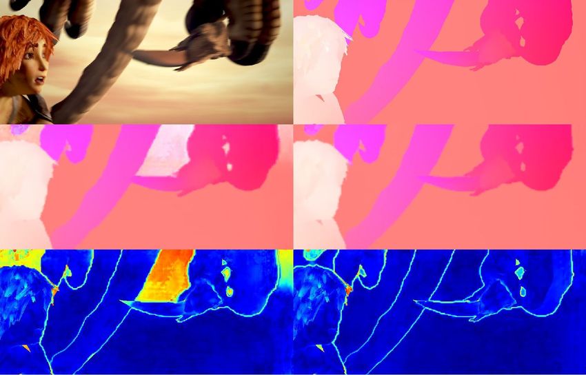
Fig. 1: Optical flow predictions from our model on images from Sintel and KITTI.
Abstract. In this work we review the coarse-to-fine spatial feature pyra-
mid concept, which is used in state-of-the-art optical flow estimation net-
works to make exploration of the pixel flow search space computationally
tractable and efficient. Within an individual pyramid level, we improve
the cost volume construction process by departing from a warping- to a
sampling-based strategy, which avoids ghosting and hence enables us to
better preserve fine flow details. We further amplify the positive effects
through a level-specific, loss max-pooling strategy that adaptively shifts
the focus of the learning process on under-performing predictions. Our
second contribution revises the gradient flow across pyramid levels. The
typical operations performed at each pyramid level can lead to noisy,
or even contradicting gradients across levels. We show and discuss how
properly blocking some of these gradient components leads to improved
convergence and ultimately better performance. Finally, we introduce a
distillation concept to counteract the issue of catastrophic forgetting dur-
ing finetuning and thus preserving knowledge over models sequentially
trained on multiple datasets. Our findings are conceptually simple and
easy to implement, yet result in compelling improvements on relevant er-
ror measures that we demonstrate via exhaustive ablations on datasets
like Flying Chairs2, Flying Things, Sintel and KITTI. We establish new
state-of-the-art results on the challenging Sintel and KITTI 2012 test
datasets, and even show the portability of our findings to different opti-
cal flow and depth from stereo approaches.
Preliminary paper version: Link to the final authenticated version to be announced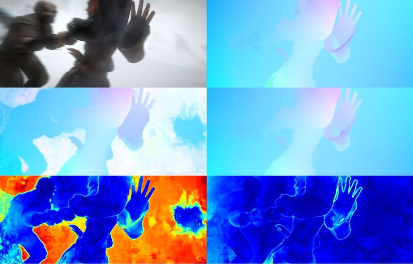
2      M. Hofinger et al.

1   Introduction
State-of-the-art, deep learning based optical flow estimation methods share a
number of common building blocks in their high-level, structural design. These
blocks reflect insights gained from decades of research in classical optical flow
estimation, while exploiting the power of deep learning for further optimization
of e.g. performance, speed or memory constraints [14,38,47]. Pyramidal repre-
sentations are among the fundamental concepts that were successfully used in
optical flow and stereo matching works like [3]. However, while pyramidal repre-
sentations enable computationally tractable exploration of the pixel flow search
space, their downsides include difficulties in the handling of large motions for
small objects or generating artifacts when warping occluded regions. Another
observation we made is that vanilla agglomeration of hierarchical information
in the pyramid is hindering the learning process and consequently leading to
reduced performance.
    In this paper we identify and address shortcomings in state-of-the-art flow
networks, with particular focus on improving information processing in the pyra-
midal representation module. For cost volume construction at a single pyramid
level, we introduce a novel feature sampling strategy rather than relying on
warping of high-level features to the corresponding ones in the target image.
Warping is the predominant strategy in recent and top-performing flow meth-
ods [47,14] but leads to degraded flow quality for fine structures. This is because
fine structures require robust encoding of high-frequency information in the fea-
tures, which is sometimes not recoverable after warping them towards the target
image pyramid feature space. As an alternative we propose sampling for cost
volume generation in each pyramid level, in conjunction with the sum of ab-
solute differences as a cost volume distance function. In our sampling strategy
we populate cost volume entries through distance computation between features
without prior feature warping. This helps us to better explore the complex and
non-local search space of fine-grained, detailed flow transformations (see Fig. 1).
    Using sampling in combination with a per-pyramid level loss max-pooling
strategy further supports recovery of the motion of small and fast-moving ob-
jects. Flow errors for those objects can be attributed to the aforementioned warp-
ing issue but also because the motion of such objects often correlates with large
and underrepresented flow vectors, rarely available in the training data. Loss
max-pooling adaptively shifts the focus of the learning procedure towards under-
performing flow predictions, without requiring additional information about the
training data statistics. We introduce a loss max-pooling variant to work in
hierarchical feature representations, while the underlying concept has been suc-
cessfully used for dense pixel prediction tasks like semantic segmentation [31].
    Our second major contribution targets improving the gradient flow across
pyramid levels. Functions like cost volume generation depend on bilinear in-
terpolation, which can be shown [20] to produce considerably noisy gradients.
Furthermore, fine-grained structures which are only visible at a certain pyramid
level, can propagate contradicting gradients towards the coarser levels when they
move in a different direction compared to their background. Accumulating these
IOFPL - Improving Optical Flow on a Pyramid Level          3

gradients across pyramid levels ultimately inhibits convergence. Our proposed
solution is as simple as effective: by using level-specific loss terms and smartly
blocking gradient propagation, we can eliminate the sources of noise. Doing so
significantly improves the learning procedure and is positively reflected in the
relevant performance measures.
    As minor contributions, we promote additional flow cues that lead to a more
effective generation of the cost volume. Inspired by the work of [15] that used
backward warping of the optical flow to enhance the upsampling of occlusions,
we advance symmetric flow networks with multiple cues (like consistencies de-
rived from forward-backward and reverse flow information, occlusion reasoning)
to better identify and correct discrepancies in the flow estimates. Finally, we also
propose knowledge distillation to counterfeit the problem of catastrophic forget-
ting in the context of deep-learning-based optical flow algorithms. Due to a lack
of large training datasets, it is common practice to sequentially perform a num-
ber of trainings, first on synthetically generated datasets (like Flying Chairs2
and Flying Things), then fine-tuning on target datasets like Sintel or KITTI.
Our distillation strategy (inspired by recent work on scene flow [19] and un-
supervised approaches [22,21]) enables us to preserve knowledge from previous
training steps and combine it with flow consistency checks generated from our
network and further information about photometric consistency.
    Our combined contributions lead to significant, cumulated error reductions
over state-of-the-art networks like HD3 or (variants of) PWC-Net [47,38,15,2],
and we set new state-of-the-art results on the challenging Sintel and KITTI
2012 datasets. We provide exhaustive ablations and experimental evaluations on
Sintel, KITTI 2012 and 2015, Flying Things and Flying Chairs2, and significantly
improve on the most important measures like Out-Noc (percentage of erroneous
non-occluded pixels) and on EPE (average end-point-error) metrics.

2   Related Work

Classical approaches. Optical flow has come a long way since it was introduced
to the computer vision community by Lucas and Kanade [24] and Horn and
Schunck [13]. Following these works, the introduction of pyramidal coarse-to-
fine warping frameworks were giving another huge boost in the performance of
optical flow computation [4,35] – an overview of non learning-based optical flow
methods can be found in [1,36,9].

Deep Learning entering optical flow. Many parts of the classical optical flow
computations are well-suited for being learned by a deep neural network. Initial
work using deep learning for flow was presented in [42], and was using a learned
matching algorithm to produce semi-dense matches then refining them with a
classical variational approach. The successive work of [30], whilst also relying
on learned semi-dense matches, was additionally using an edge detector [7] to
interpolate dense flow fields before the variational energy minimization. End-to-
end learning in a deep network for flow estimation was first done in FlowNet [8].
4      M. Hofinger et al.

They use a conventional encoder-decoder architecture, and it was trained on a
synthetic dataset, showing that it still generalizes well to real world datasets
such as KITTI [11]. Based on this work, FlowNet2 [16] improved by using a
carefully tuned training schedule and by introducing warping into the learning
framework. However, FlowNet2 could not keep up with the results of traditional
variational flow approaches on the leaderboards. SpyNet[28] introduced spatial
image pyramids and PWC-Net [37,38] additionally improved results by incorpo-
rating spatial feature pyramid processing, warping, and the use of a cost volume
in the learning framework. The flow in PWC-Net is estimated by using a stack of
flattened cost volumes and image features from a Dense-Net. In [15], PWC-Net
was turned into an iterative refinement network, adding bilateral refinement of
flow and occlusion in every iteration step. ScopeFlow [2] showed that improve-
ments on top of [15] can be achieved simply by improving training procedures.
In the work of [29], the group around [37] was showing further improvements
on Kitti 2015 and Sintel by integrating the optical flow from an additional, pre-
vious image frame. While multi-frame optical flow methods already existed for
non-learning based methods [6,44,10], they were the first to show this in a deep
learning framework. In [47], the hierarchical discrete distribution decomposi-
tion framework HD3 learned probabilistic pixel correspondences for optical flow
and stereo matching. It learns the decomposed match densities in an end-to-end
manner at multiple scales. HD3 then converts the predicted match densities into
point estimates, while also producing uncertainty measures at the same time.
Devon [23] uses a sampling and dilation based deformable cost-volume, to iter-
atively estimate the flow at a fixed quarter resolution in each iteration. While
they showed good results on clean synthetic data, the performance on real images
from KITTI was sub-optimal, indicating that sampling alone may not be suffi-
cient. We will show here, that integrating a direct sampling based approach into
a coarse-to-fine pyramid together with LMP and Flow Cues can actually lead to
very good results. Recently, Volumetric Correspondence Networks (VCN) [46]
showed that the 4D cost volume can also be efficiently filtered directly without
the commonly used flattening but using separable 2D filters instead.

Unsupervised methods. Generating dense and accurate flow data for supervised
training of networks is a challenging task. Thus, most large-scale datasets are
synthetic [5,8,17], and real data sets remained small and sparsely labeled [27,26].
Unsupervised methods do not rely on that data, instead, those methods usually
utilize the photometric loss between the original image in the warped, second
image to guide the learning process [48]. However, the photometric loss does not
work for occluded image regions, and therefore methods have been proposed to
generate occlusion masks beforehand or simultaneously [25,45].

Distillation. To learn the flow values of occluded areas, DDFlow [21] is using a
student-teacher network which distills data from reliable predictions, and uses
these predictions as annotations to guide a student network. SelFlow [22] is
built in a similar fashion but vastly improves the quality of the flow predictions
in occluded areas by introducing a superpixel-based occlusion hallucination tech-
IOFPL - Improving Optical Flow on a Pyramid Level           5

nique. They obtain state-of-the-art results when fine-tuning on annotated data
after pre-training in a self-supervised setting. SENSE [19] tries to integrate op-
tical flow, stereo, occlusion, and semantic segmentation in one semi-supervised
setting. Much like in a multi-task learning setup, SENSE [19] uses a shared en-
coder for all four tasks, which can exploit interactions between the different tasks
and leads to a compact network. SENSE uses pre-trained models to “supervise”
the network on data with missing ground truth annotations using a distillation
loss [12]. To couple the four tasks, a self-supervision loss term is used, which
largely improves regions without ground truth (e.g. sky regions).

3     Main Contributions
In this section we review pyramid flow network architectures [37,47], and propose
a set of modifications to the pyramid levels (§ 3.2) and their training strategy
(§ 3.3), which work in a synergistic manner to greatly boost performance.

3.1   Pyramid flow networks
Pyramid flow networks (PFN) operate on pairs of images, building feature pyra-
mids with decreasing spatial resolution using “siamese” network branches with
shared parameters. Flow is iteratively refined starting from the top of the pyra-
mid, each layer predicting an offset relative to the flow estimated at the previous
level. For more details about the operations carried out at each level see § 3.2.

Notation. We represent multi-dimensional feature maps as functions Iil : Iil →
Rd , where i = 1, 2 indicates which image the features are computed from, l is
their pyramid level, and Iil ⊂ R2 is the set of pixels of image i at resolution l.
                                                l
We call forward flow at level l a mapping F1→2       : I1l → R2 , which intuitively
                             l              l
indicates where pixels in I1 moved to in I2 (in relative terms). We call backward
                       l
flow the mapping F2→1       : I2l → R2 that indicates the opposite displacements.
Pixel coordinates are indexed by u and v, i.e. x = (xu , xv ), and given x ∈ I1l , we
assume that I1l (x) implicitly applies bilinear interpolation to read values from
I1l at sub-pixel locations.

3.2   Improving pyramid levels in PFNs
Many PFNs [37,47] share the same high-level structure in each of their levels.
First, feature maps from the two images are aligned using the coarse flow esti-
mated in the previous level, and compared by some distance function to build a
cost volume (possibly both in the forward and backward directions). Then, the
cost volume is combined with additional information from the feature maps (and
optionally additional “flow cues”) and fed to a “decoder” subnet. This subnet fi-
nally outputs a residual flow, or a match density from which the residual flow
can be computed. A separate loss is applied to each pyramid layer, providing
deep supervision to the flow refinement process. In the rest of this section, we
describe a set of generic improvements that can be applied to the pyramid layers
of several state of the art pyramid flow networks.
6       M. Hofinger et al.

                                                                                                                                    (warp)
       I1              I2              I2→1

                                                   a)

                                                                    Pyramid                                             Warping:
                                                                                                                        Transforms image
                                                                     levels                                -1,est
                                                                                                                        leads to ghosting,

                                                   b)                                                                   Sample: Flow
                                                                                                                         only shifts gray
                                                                                                                         search window
                                                                                                                         for black dot

                                                   c)
                                                             +                                      +                        +
                                                        0 1 2 3 4      0 1 2 3 4   +(sample)   0 1 2 3 4
                                                                                                           -1,est, up
                                                                                                                        0 1 2 3 4
                                                                                                                                    (warp)

Fig. 2: Sampling vs. Warping. Left: Warping leads to image ghosting in the
warped image I2→1 ; Also, neighbouring pixels in I1 must share parts of their
search windows in I2→1 , while for sampling they are independently sampled
from the original image I2 . Right: A toy example; a) Two moving objects: a
                                                             gt
red line with a black dot and a blue box. Warping with F1→2      leads to ghosting
effects. b) Zooming into lowest pyramid resolution shows loss of small details
due to down-scaling. c) Warping I2l with the flow estimate from the coarser
                               l
level leads to distortions in I2→1 (the black dot gets covered up). Instead, direct
               l
sampling in I2 with a search window(gray box) that is offset by the flow estimate
avoids these distortions and hence leads to more stable correlations.

Cost volume construction The first operation at each level of most pyramid
flow networks involves comparing features between I1l and I2l , conditioned on the
       l−1
flow F1→2  predicted at the previous level. In the most common implementation,
  l                 l−1
I2 is warped using F1→2 , and the result is cross-correlated with I1l . More formally,
        l       l−1                                      l                     l−1
given I2 and F1→2 , the warped image is given by I2→1       (x) = I2l (x + F1→2    (x))
and the cross-correlation is computed with:
        warp                                                           l−1
      V1→2   (x, δ) = I1l (x) · I2→1
                                 l
                                     (x + δ) = I1l (x) · I2l (x + δ + F1→2 (x + δ)) ,                                                  (1)

where δ ∈ [−∆, ∆]2 is a restricted search space and · is the vector dot product.
This warping operation, however, suffers from a serious drawback which occurs
when small regions move differently compared to their surroundings.
    This case is represented in Fig. 2: A small object indicated by a red line moves
in a different direction than a larger blue box in the background. As warping
uses the coarse flow estimate from the previous level, which cannot capture
fine-grained motions, there is a chance that the smaller object gets lost during
                                                         l
the feature warping. This makes it undetectable in I2→1      , even with an infinite
cost volume range (CVr/CV-range) δ. To overcome this limitation, we propose
a different cost volume construction strategy, which exploits direct sampling
operations. This approach always accesses the original, undeformed features I2l ,
without loss of information, and the cross-correlation in Eq. (1) now becomes:
                    samp,Corr                                  l−1
                  V1→2        (x, δ) = I1l (x) · I2l (x + δ + F1→2 (x)) .                                                              (2)

For this operator, the flow just acts as an offset that sets the center of the
correlation window in the feature image I2l . Going back to Fig. 2, one can see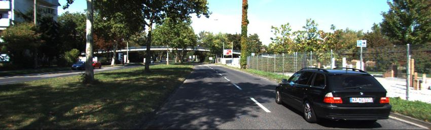
IOFPL - Improving Optical Flow on a Pyramid Level            7

HD3
Ours           End point error                             Optical Flow

Fig. 3: Predicted optical flow and end point error on KITTI obtained with HD3
from the model zoo (top) and our IOFPL version (bottom). Note how our model
is better able to preserve small details.

that the sampling operator is still able to detect the small object, as it is also
exemplified on real data in Fig. 3. In contrast to [23], our approach still uses the
coarse to fine pyramid and hence doesn’t require dilation in the cost volume for
large motions. In our experiments we also consider a variant where the features
are compared in terms of Sum of Absolute Differences (SAD) instead of a dot
product:
                 samp,SAD                                   l−1
               V1→2       (x, δ) = kI1l (x) − I2l (x + δ + F1→2 (x))k1 .         (3)

Loss Max Pooling We apply a Loss Max-Pooling (LMP) strategy [31], also
known as Online Hard Example Mining (OHEM), to our knowledge for the first
time in the context of optical flow. In our experiments, and consistent with the
findings in [31], we observe that LMP can help to better preserve small details
in the flow. The total loss is the sum of a pixelwise loss `x over all x ∈ I1 , but we
optimize a weighted version thereof that selects a fixed percentage of the highest
per-pixel losses. The percentage value α is best chosen according to the quality
of the ground-truth in the target dataset. This can be written in terms of a loss
max-pooling strategy as follows:
                         (                                           )
                           X                                    1
               L = max           wx `x : kwk1 ≤ 1 , kwk∞ ≤             ,            (4)
                                                              α|I1 |
                           x∈I1

which is equivalent to putting constant weight wx = α|I1 1 | on the percentage of
pixels x exhibiting the highest losses, and setting wx = 0 elsewhere.
    LMP lets the network focus on the more difficult areas of the image, while
reducing the amount of gradient signals where predictions are already correct. To
avoid focussing on outliers, we set the loss to 0 for pixels that are out of reach
for the current relative search range ∆. For datasets with sparsely annotated
ground-truth, like e.g. KITTI [11], we re-scale the per pixel losses `x to reflect
the number of valid pixels. Note that, when performing distillation, loss max-
pooling is only applied to the supervised loss, in order to further reduce the
effect of noise that survived the filtering process described in § 3.4.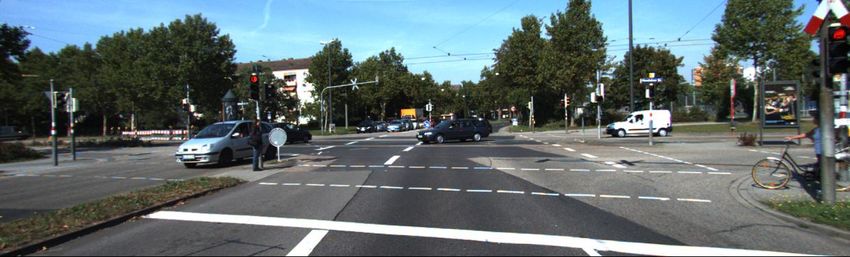
8       M. Hofinger et al.

3.3   Improving gradient flow across PFN levels
Our quantitatively most impacting contribution relates to the way we pass gra-
dient information across the different levels of a PFN. In particular, we focus
on the bilinear interpolation operations that we implicitly perform on I2l while
computing Eq.s (1), (2) and (3). It has been observed [20] that taking the gradi-
                                                                                 l−1
ent of bilinear interpolation w.r.t. the sampling coordinates (i.e. the flow F1→2
from the previous level in our case) is often problematic. To illustrate the reason,
we restrict our attention to the 1-D case for ease of notation, and write linear
interpolation from a function fˆ : Z → R:
                           X
                  f (x) =       fˆ(bxc + η) [(1 − η)(1 − x̃) + ηx̃] ,             (5)
                         η∈{0,1}

where x̃ = x − bxc denotes the fractional part of x. The derivative of the inter-
polated function f (x) with respect to x is:
                        df       X
                           (x) =   fˆ(bxc + η)(2η − 1) .                                    (6)
                        dx
                                   η∈{0,1}

                          df
The gradient function dx     is discontinuous, for its value drastically changes as
bxc crosses over from one integer value to the next, possibly inducing strong
noise in the gradients. An additional effect, specific to our case, is related to the
                                              l−1
issues already highlighted in § 3.2: since F1→2    is predicted at a lower resolution
than level l operates at, it cannot fully capture the motion of smaller objects.
When this motion contrasts with that of the background, the gradient w.r.t.
  l−1
F1→2   produced from the sampling at level l will inevitably disagree with that
produced by the loss at level l − 1, possibly slowing down convergence.
    While [20] proposes a different sampling strategy to reduce the noise issues
discussed above, in our case we opt for a much simpler work around. Given
the observations about layer disagreement, and the fact that the loss at l − 1
                                           l−1
already provides direct supervision on F1→2    , we choose to stop back-propagation
of partial flow gradients coming from higher levels, as illustrated in Fig. 4.
    Evidence for this effect can be seen in Fig. 5, where the top shows the develop-
ment of the training loss for a Flying Chairs 2 training with an HD3 model. The

                Cost                                    Cost volume construction: warping
                               Decoder        to loss
               Volume
                                                                           Build CV
                                                                Warp
                        Flow        gradient stopped
                        Cues                            Cost volume construction: sampling

                                                                    Build CV
                Cost           Decoder        to loss             with Sampling
               Volume

Fig. 4: Left: Network structure – flow estimation per pyramid level; Gradients are
stopped (red cross); Right: Cost volume computation with sampling vs. warping.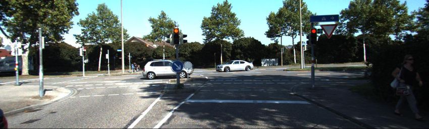
IOFPL - Improving Optical Flow on a Pyramid Level                                  9

                                 4
                                                                                                                 Loss, baseline
                    Loss train                                                                                   Loss gradient-stopping
                                 2

                       0.50
 NCC of gradients

                                         NCC,level=0   NCC,level=1    NCC,level=2   epochs NCC,level=3

                       0.0

                    −0.5
                                     0          25        50         75              100             125   150         175            200
                                                                                    epochs
Fig. 5: Top: Loss of model decreases when the flow gradient is stopped; Bottom:
Partial gradients coming from the current level loss and the next level via the
flow show a negative Normalized Cross Correlation (NCC), indicating that they
oppose each other.

training convergence clearly improves when the partial flow gradient is stopped
between the levels (red cross in Fig. 4). On the bottom of the figure the Normal-
ized Cross Correlation (NCC) between the partial gradient coming from the next
level via the flow and the current levels loss is shown. On average the correlation
is negative, indicating that for each level of the network the partial gradient that
we decided to stop (red cross), coming from upper levels, points in a direction
that opposes the partial gradient from the loss directly supervising the current
level, thus harming convergence. Additional evidence of the practical, positive
impact of our gradient stopping strategy is given in the experiment section § 4.2.
    Further evidence on this issue can be gained by analyzing the parameters
gradient variance [40] as it impacts the rate of convergence for stochastic gradient
descent methods. Also the β-smoothness [34] of the loss function gradient can
give similar insights. In the supplementary material (section § A) we provide
further experiments that show that gradient stopping also helps to improve these
properties, and works for stereo estimation and other flow models as well.

3.4                              Additional refinements
Flow cues As mentioned at the beginning of § 3.2, the decoder subnet in each
pyramid level processes the raw feature correlations to a final cost volume or
direct flow predictions. To provide the decoder with contextual information, it
commonly [37,47] also receives raw features (i.e. I1l , I2l for forward and backward
flow, respectively). Some works [41,15,17] also append other cues, in the form of
hand-crafted features, aimed at capturing additional prior knowledge about flow
consistency. Such flow cues are cheap to compute but otherwise hard to learn for
CNNs as they require various forms of non-local spatial transformations. In this
work, we propose a set of such flow cues that provides mutual beneficial informa-
tion, and perform very well in practice when combined with costvolume sample
and LMP (see § 4.2). These cues are namely forward-backward flow warping, re-
verse flow estimation, map uniqueness density and out-of-image occlusions, and
are described in detail in the supplementary material (§ B).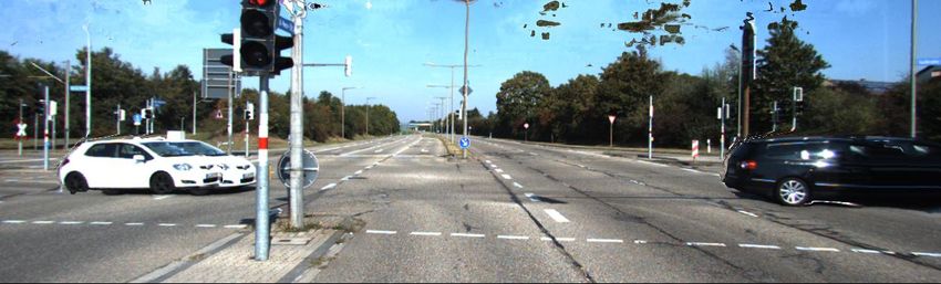
10 M. Hofinger et al.
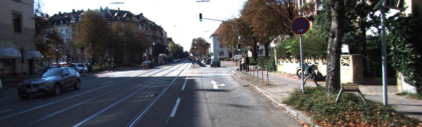
I1 KITTI GT
Inference after Things3D distilled pseudo GT
Fig. 6: Illustration of our data distillation process. Left to right: input image
and associated KITTI ground truth, dense prediction from a Flying Things3D-
trained network and pseudo-ground truth derived from it.
Knowledge distillation Knowledge distillation [12] consists in extrapolating
a training signal directly from another trained network, ensemble of networks,
or perturbed networks [32], typically by mimicking their predictions on some
available data. In PFNs, distillation can help to overcome issues such as lack of
flow annotations on e.g. sky, which results in cluttered outputs in those areas.
Formally, our goal is to distill knowledge from a pre-trained master network (e.g.
on Flying Chairs2 and/or Flying Things) by augmenting a student network with
an additional loss term, which tries to mimic the predictions the master produces
on the input at hand (Fig. 6, bottom left). At the same time, the student is also
trained with a standard, supervised loss on the available ground-truth (Fig. 6, top
right). In order to ensure a proper cooperation between the two terms, we prevent
the distillation loss from operating blindly, instead enabling it selectively based
on a number of consistency and confidence checks (refer to the supplementary
material for details). Like for the ground-truth loss, the data distillation loss is
scaled with respect to the valid pixels present in the pseudo ground-truth. The
supervised and the distillation losses are combined into a total loss
L = αLS + (1 − α)LD (7)
with the scaling factor α = 0.9. A qualitative representation of the effects of our
proposed distillation on KITTI data is given in Fig. 7.
4 Experiments
We assess the quality of our contributions by providing a number of exhaustive
ablations on Flying Chairs, Flying Chairs2, Flying Things, Sintel, Kitti 2012 and
Kitti 2015. We ran the bulk of ablations based on HD3 [47], i.e. a state-of-the-
art, 2-frame optical flow approach. We build on top of their publicly available
code and stick to default configuration parameters where possible, and describe
and re-train the baseline model when deviating.IOFPL - Improving Optical Flow on a Pyramid Level 11
I2→1(x)
F2→1(x) error HD3 Modelzoo Ours Ours Distilled
Fig. 7: Qualitative results on KITTI for: HD3 modelzoo (left), our version with
all contributions except distillation (center), and with distillation (right).
The remainder of this section is organized as follows. We provide i) in § 4.1
a summary about the experimental and training setups and our basic modifi-
cations over HD3 , ii) in § 4.2 an exhaustive number of ablation results for all
aforementioned datasets by learning only on the Flying Chairs2 training set,
and for all reasonable combinations of our contributions described in § 3, as well
as ablations on Sintel, and iii) list and discuss in § 4.3 our results obtained on the
Kitti 2012, Kitti 2015 and Sintel test datasets, respectively. In the supplementary
material we further provide i) more technical details and ablation studies about
the used flow cues, ii) smoothness and variance analyses for gradient stopping
and its impact on depth from stereo or with a PWC baseline iii) ablations on
extended search ranges for the cost volume, and iv) ablations on distillation.
4.1 Setup and modifications over HD3
We always train on 4xV100 GPUs with 32GB RAM using PyTorch, and obtain
additional memory during training by switching to In-Place Activated Batch-
Norm (non-synchronized, Leaky-ReLU) [33]. We decided to train on Flying
Chairs2 rather than Flying Chairs for our main ablation experiments, since it
provides ground truth for both, forward and backward flow directions. Other
modifications are experiment-specific and described in the respective sections.
Flow - Synthetic data pre-training. Also the Flying Things dataset provides
ground truth flow for both directions. We always train and evaluate on both
flow directions, since this improves generalization to other datasets. We use a
batch size of 64 to decrease training times and leave the rest of configuration
parameters unchanged w.r.t. the default HD3 code.
Flow - Fine-tuning on KITTI. Since both the Kitti 2012 and the Kitti 2015
datasets are very small and only provide forward flow ground truth, we follow
the HD3 training protocol and join all KITTI training sequences for the final
fine-tuning (after pre-training on Flying Chairs2 and Flying Things). However,
we ran independent multi-fold cross validations and noticed faster convergence12 M. Hofinger et al.
Table 1: Ablation results when training HD3 CVr±4 on Flying Chairs2 v.s.
the official model zoo baseline, our re-trained baseline and when adding all our
proposed contributions. Results are shown on validation data for Flying Chairs2
and Flying Things (validation set used in the original HD3 code repository), and
on the official training data for Sintel, Kitti 2012 and Kitti 2015, due to the lack
of a designated validation split. (Highlighting best and second-best results).
Gradient Sampling Flow SAD LMP Flying Chairs2 Flying Things Sintel final Sintel clean Kitti 2012 Kitti 2015
Stopping Cues EPE [1] Fl-all [%] EPE [1] Fl-all [%] EPE [1] Fl-all [%] EPE [1] Fl-all [%] EPE [1] Fl-all [%] EPE [1] Fl-all [%]
HD3 baseline model zoo 1.439 7.17 20.973 33.21 5.850 14.03 3.70 8.56 12.604 49.13 22.67 57.07
HD3 baseline – re-trained 1.422 6.99 17.743 26.72 6.273 15.24 3.90 10.04 8.725 34.67 20.98 50.27
3 7 7 7 7 1.215 6.23 19.094 26.84 5.774 15.89 3.72 10.51 9.469 44.58 19.07 53.65
3 7 3 7 7 1.216 6.24 16.294 26.25 6.033 16.26 3.43 9.98 7.879 43.92 17.97 51.14
3 3 7 7 7 1.208 6.19 17.161 24.75 6.074 15.61 3.70 9.96 8.673 45.29 17.42 51.23
3 3 3 7 7 1.186 6.16 19.616 28.51 7.420 15.99 3.61 9.39 6.672 32.59 16.23 47.56
3 3 3 3 7 1.184 6.15 15.136 25.00 5.625 16.35 3.38 9.97 8.144 41.59 17.13 52.51
3 7 7 7 3 1.193 6.02 44.068 40.38 12.529 17.85 5.48 10.95 8.778 42.37 19.08 51.13
3 3 3 7 3 1.170 5.98 15.752 24.26 5.943 16.27 3.55 9.91 7.742 35.78 18.75 49.67
3 3 3 3 3 1.168 5.97 14.458 23.01 5.560 15.88 3.26 9.58 6.847 35.47 16.87 49.93
of our model over the baseline. We therefore perform early stopping after 1.6k
(CVr±4)/ 1.4k (CVr±8) epochs, to prevent over-fitting. Furthermore, before
starting the fine-tuning process of the pre-trained model, we label the KITTI
training data for usage described in the knowledge distillation paragraph in § 3.4.
Flow - Fine-tuning on Sintel. We only train on all the images in the final pass
and ignore the clean images like HD3 for comparability. Also, we only use the
forward flow ground truth since backward flow ground truth is unavailable. Al-
though not favorable, our model can still be trained in this setting since we
use a single, shared set of parameters for the forward and the backward flow
paths. We kept the original 1.2k finetuning iterations for comparability, since
our independent three-fold cross validation did not show signs of overfitting.
4.2 Flow ablation experiments
Here we present an extensive number of ablations based on HD3 to assess the
quality of all our proposed contributions. We want to stress that all results in
Tab. 1 were obtained by solely training on the Flying Chairs2 training
set. More specifically, we report error numbers (EPE and Fl-all; lower is better)
and compare the original HD3 model zoo baseline against our own, retrained
baseline model, followed by adding combinations of our proposed contributions.
We report performance on the target domains validation set (Flying Chairs2),
as well as on unseen data from different datasets (Flying Things, Sintel and
KITTI), to gain insights on generalization behavior.
Our ablations show a clear trend towards improving EPE and Fl-all, espe-
cially on the target domain, as more of our proposed improvements are inte-
grated. Due to the plethora of results provided in the table, we highlight some
of them next. Gradient stopping is often responsible for a large gap w.r.t. to
both baseline HD3 models, the original and our re-trained. Further, all variants
with activated Sampling lead to best- or second-best results, except for Fl-all
on Sintel. Flow Cues give an additional benefit when combined with SamplingIOFPL - Improving Optical Flow on a Pyramid Level 13
Table 2: Ablation results on Sintel, highlighting best and second-best results.
Top: Baseline and Flying Chairs2 & Flying Things pre-trained (P) models only.
Bottom: Results after additional fine-tuning (F) on Sintel.
Fine-tuned Gradient Sampling Flow SAD LMP CV Flying Things Sintel final Sintel clean
Pretrained Stopping Cues range ±8 EPE [1] Fl-all EPE [1] Fl-all EPE [1] Fl-all
HD3 baseline – re-trained 12.52 18.06% 13.38 16.23 % 3.06 6.39%
P 3 7.98 13.41% 4.06 10.62 % 1.86 5.11%
P 3 3 3 3 3 7.06 12.29% 4.23 11.05 % 2.20 5.41%
P 3 3 3 3 3 3 5.77 11.48% 4.68 11.40 % 1.77 4.88%
F 19.89 27.03% (1.07) (4.61 %) 1.58 4.67%
F 3 13.80 20.87% (0.84) (3.79 %) 1.43 4.19%
F 3 3 3 3 3 14.19 20.98% (0.82) (3.63 %) 1.43 4.08%
F 3 3 3 3 3 3 11.80 19.12% (0.79) (3.49 %) 1.19 3.86%
but not with warping. Another relevant insight is that our full model using all
contributions at the bottom of the table always improves on Fl-all compared
to the variant with deactivated LMP. This shows how LMP is suitable to ef-
fectively reduce the number of outliers by focusing the learning process on the
under-performing (and thus more rare) cases.
We provide additional ablation results on Flying Things and Sintel in Tab. 2.
The upper half shows PreTrained (P) results obtained after training on Flying
Chairs2 and Flying Things, while the bottom shows results after additionally
fine-tuning (F) on Sintel. Again, there are consistent large improvements on
the target domain currently trained on, i.e. (P) for Flying Things and (F) for
Sintel. On the cross dataset validation there is more noise, especially for sintel
final that comes with motion blur etc., but still always a large improvement over
the baseline. After finetuning (F) the full model with CVr±8 shows much better
performance on sintel and at the same time comparable performance on Flying
Things to the original baseline model directly trained on Flying Things.
4.3 Optical flow benchmark results
The following provides results on the official Sintel and KITTI test set servers.
Sintel. By combining all our contributions and by using a cost volume search
range of ±8, we set a new state-of-the-art on the challenging Sintel Final test
set, improving over the very recent, best-working approach in [2] (see Tab. 3).
Even by choosing the default search range of CVr±4 as in [47] we still obtain
significant improvements over the HD3 -ft baseline on training and test errors.
Kitti 2012 and Kitti 2015. We also evaluated the impact of our full model on
KITTI and report test data results in Tab. 4. We obtain new state-of-the-art
test results for EPE and Fl-all on Kitti 2012, and rank second-best at Fl-all on
Kitti 2015. On both, Kitti 2012 and Kitti 2015 we obtain strong improvements
on the training set on EPE and Fl-all. Finally, while on Kitti 2015 the recently
published VCN [46] has slightly better Fl-all scores, we perform better on fore-
ground objects (test Fl-fg 8.09 % vs. 8.66 %) and generally improve over the14 M. Hofinger et al.
Table 3: EPE scores on the Sin- Table 4: EPE and Fl-all scores on the KITTI
tel test datasets. The appendix -ft test datasets. The appendix -ft denotes fine-
denotes fine-tuning on Sintel. tuning on KITTI. Ours is IOFPL.
Training Test Kitti 2012 Kitti 2015
Method Clean Final Clean Final Method EPE EPE Fl-noc [%] EPE Fl-all [%] Fl-all [%]
train test test train train test
FlowNet2 [16] 2.02 3.14 3.96 6.02
FlowNet2-ft [16] (1.45) (2.01) 4.16 5.74 FlowNet2 [16] 4.09 - - 10.06 30.37 -
PWC-Net [37] 2.55 3.93 - - FlowNet2-ft [16] (1.28) 1.8 4.82 (2.30) 8.61 10.41
PWC-Net-ft [37] (2.02) (2.08) 4.39 5.04 PWC-Net [37] 4.14 - - 10.35 33.67 -
SelFlow [22] 2.88 3.87 6.56 6.57 PWC-Net-ft [37] (1.45) 1.7 4.22 (2.16) 9.80 9.60
SelFlow-ft [22] (1.68) (1.77) 3.74 4.26 SelFlow [22] 1.16 2.2 7.68 (4.48) - 14.19
IRR-PWC-ft [15] (1.92) (2.51) 3.84 4.58 SelFlow-ft [22] (0.76) 1.5 6.19 (1.18) - 8.42
IRR-PWC-ft [15] - - - (1.63) 5.32 7.65
PWC-MFF-ft [29] - - 3.42 4.56
PWC-MFF-ft [29] - - - - - 7.17
VCN-ft [46] (1.66) (2.24) 2.81 4.40
ScopeFlow [2] - 1.3 2.68 - - 6.82
ScopeFlow [2] - - 3.59 4.10
Devon [23] - - 6.99 - 14.31
Devon [23] - - 4.34 6.35
VCN [46] - - - (1.16) 4.10 6.30
HD3 [47] 3.84 8.77 - -
HD3F [47] 4.65 - - 13.17 23.99
HD3 -ft [47] (1.70) (1.17) 4.79 4.67
HD3F-ft [47] (0.81) 1.4 2.26 1.31 4.10 6.55
IOFPL-no-ft 2.20 4.32 - - IOFPL-no-ft 2.52 - - 8.32 20.33 -
IOFPL-ft 1.43 (0.82) 4.39 4.22 IOFPL-ft (0.73) 1.2 2.29 1.17 3.40 6.52
IOFPL-CVr8-no-ft 1.77 4.68 - - IOFPL-CVr8-no-ft 2.37 - - 7.09 18.93 -
IOFPL-CVr8-ft 1.19 (0.79) 3.58 4.01 IOFPL-CVr8-ft (0.76) 1.2 2.25 1.14 3.28 6.35
HD3 baseline (Fl-fg 9.02 %). It is worth noting that all KITTI finetuning results
are obtained after integrating knowledge distillation from § 3.4, leading to sig-
nificantly improved flow predictions on areas where KITTI lacks training data
(e.g. in far away areas including sky, see Fig. 7). We provide further qualitative
insights and direct comparisons in the supplementary material (§ C).
5 Conclusions
In this paper we have reviewed the concept of spatial feature pyramids in context
of modern, deep learning based optical flow algorithms. We presented comple-
mentary improvements for cost volume construction at a single pyramid level,
that i) departed from a warping- to a sampling-based strategy to overcome is-
sues like handling large motions for small objects, and ii) adaptively shifted
the focus of the optimization towards under-performing predictions by means
of a loss max-pooling strategy. We further analyzed the gradient flow across
pyramid levels and found that properly eliminating noisy or potentially contra-
dicting ones improved convergence and led to better performance. We applied
our proposed modifications in combination with additional, interpretable flow
cue extensions as well as distillation strategies to preserve knowledge from (syn-
thetic) pre-training stages throughout multiple rounds of fine-tuning. We exper-
imentally analyzed and ablated all our proposed contributions on a wide range
of standard benchmark datasets, and obtained new state-of-the-art results on
Sintel and Kitti 2012.
Acknowledgements: T. Pock and M. Hofinger acknowledge that this work was
supported by the ERC starting grant HOMOVIS (No. 640156).IOFPL - Improving Optical Flow on a Pyramid Level 15
Improving Optical Flow on a Pyramid Level –
Supplementary Material
This document contains supplementary material for the paper ’Improving Op-
tical Flow on a Pyramid Level’. The structure of this supplementary document
is the following:
– Further insights and experiments on gradient stopping:
• Variance analysis
• Smoothness analysis
• Cross-task evaluation - stereo
• Cross-architecture evaluation - PWC
– Details on Flow Cues:
• Notation
• Detailed explanation
• Ablations on flow cues
– Further Analysis:
• Ablation on Data distillation
• Ablation on extending search range
• Qualitative comparisons of validation epe changes
• Histograms of errors
• Qualitative training results for KITTI (images)
• Qualitative training results for MPI-Sintel (images)
• Qualitative Results on KITTI
• Qualitative Results on MPI-Sintel
• Sidenote on D2V and V2D operation with warping vs. sampling
A Further insights on Gradient Stopping
In this section we provide additional empirical insights to what is described in
Section 3.3 in the main submission document, i.e., why stopping the optical
flow gradients between the levels is beneficial. We will do this by showing that
the variance of the model parameter gradients over the training set is reduced
(sec A.1), and the Lipschitzness of the parameter gradients is improved as well,
while still providing a descent direction (sec A.2). For stochastic gradient descent
methods these properties lead to improved convergence, which is what we already
observed in the main paper (Fig. 5). Finally, we show that gradient stopping also
leads to improved convergence for the different task of stereo estimation (sec A.3)
as well as for a different architecture like PWC-Net (implemented in a different
code-base (sec A.4 ).
Preliminary paper version: Link to the final authenticated version to be announced16 M. Hofinger et al.
A.1 Gradient stopping - variance analysis
It is known [40] that for stochastic gradient descent methods the rate of con-
vergence decreases with increasing variance of the gradients over the training
set. We can show empirically that stopping the optical flow gradients between
levels (see Fig. 4 in the main paper) leads to a reduced variance of the gradients
w.r.t the whole training dataset when compared to the baseline model. To ensure
a fair and valid comparison, both model versions use identical parameters Θ and
are fed with the exact same data batches ξn all the time. The variance over each
epoch is computed independently for every single parameter using Welford’s on-
line variance computation algorithm [43] in a numerically stable variant. After
each epoch, the mean of these P single parameter variances is computed for each
model as
1 X
σ2 = VARWelford (∇fθ (ξn )) (8)
P n∈N
θ∈Θ
and shown in Fig. 8. After gradient variances are computed a standard training
is performed for 1 epoch, and the parameters of both models are update with
the new parameters of the baseline model to ensure that the only difference in
the gradient variance comes from the gradient computation itself. As can be
seen in Fig. 8 our proposed partial gradient stopping truly reduces the gradient
variance w.r.t the model parameters and the training dataset. This leads to the
improved rate of convergences for our proposed partial gradient stopping over
the baseline.
−7
8 ×10
6
4
2 baseline
gradient stopped
0
var(baseline)/var(gradient stopped)
1.6
1.4
1.2
1.0
0 10 20 30 40 50
epochs
Fig. 8: Gradient variance for a HD3 baseline model vs. a model with the proposed
gradient stopping. The baseline has a higher gradient variance over the training
data, which leads to slower convergence.IOFPL - Improving Optical Flow on a Pyramid Level 17
A.2 Gradient stopping - smoothness analysis
Here we will show that stopping the partial optical-flow gradient between the
levels also leads to a better Lipschitzness of the gradients of the loss also known
as β-smoothness, while still providing a descent direction. It is well known that
the rate of convergence increases if the function has a low curvature which cor-
responds to a low β-smoothness. We follow the approach of [34] that estimate
’effective’ β-smoothness (βeff ) by measuring the l2 gradient change over difference
in parameters, as they move along the gradient direction in the optimization.
k∇f (ξ, Θ1 ) − ∇f (ξ, Θ2 )k2
βeff = (9)
kΘ1 − Θ2 k2
We ensure a fair comparison between the baseline model and our version with
partial flow gradient stopping by evaluating the gradient functions with the
exact same parameters Θi and data batches ξn for both model versions at all
times. Fig. 9 (top) shows that on average βeff is lower which corresponds to
20 mean(βef f,baseline)
mean(βef f,gradient stopped )
10
1.0 0 10 20 30 40 50 60 70
0.5
mean(βef f,baseline > βef f,gradient stopped )
0.0
1 0 10 20 30 40 50 60 70
0
mean(N CC(∇fbaseline, ∇fgradient stopped ))
−1
0 10 20 30 40 50 60 70
epoch
Fig. 9: Partial gradient stopping vs. Lipschitzness of gradients. Top: Average of
the effective β-smoothness shows that model with gradient stopping is smoother
(lower βef f ) than the baseline; Middle: Percentage of how often gradient stopping
leads to smoother results; Bottom: Positive normalized cross correlation between
the model parameter gradients indicates that it is still a descent direction.
a lower curvature. This is confirmed by the center plot that directly compares
βeff for both models in every iteration before averaging the result. The lower
plot shows that the normalized cross correlation (NCC) of the gradients for
the parameters of both models are positively correlated. This is in contrast to
the NCC of the partial optical flow gradients (Fig. 5, main paper) between
the levels. Therefore, stopping the partial optical flow gradients between the
levels, reduces intermediate parts that oppose each other, which in turn leads
to better final gradients at the model parameters. The latter are still positively18 M. Hofinger et al.
correlated with the original parameter gradients, which shows that they still
provide a descent direction, but with better convergence properties, as shown by
our various insights. Finally, based on these analyses and the improved results
obtained in our experimental section we conclude the importance of blocking
partial optical flow gradients across levels in a pyramidal setting for improved
convergence.
A.3 Gradient stopping on depth estimation – HD3 , depth from
Stereo.
With this experiment we show that stopping the partial optical flow gradients
between the levels also works for stereo estimation. We use the Stereo training
setup of HD3 in their original publicly available codebase3 and run a training
on the Flying Things Stereo dataset. We choose to use the original version of
the code base just with gradient stopping added, and keep the original training
procedure that trains only on the left disparity. We do this to show that the
effect of gradient stopping is not just limited to the simultaneous forward and
backward training used in the main paper, but is a more general one.
Again, we find significant improvements with our proposed partial flow gradi-
ent stopping, as can be seen in Fig. 10, which leads to an improvement of ≈10%
on the final EPE. This confirms that gradient stopping also works for stereo
estimation networks. Furthermore, it verifies that gradient stopping does not
require joint forward- and backward flow training as used in the flow ablations
in the main paper, but also leads to significant gains for a standard forward-only
training.
2.4
EPE Endpoint error [pixel]
2.2 Baseline
2.0 Baseline + Gradient Stopped
1.8
1.6
1.4
1.2
1.0 0 25 50 75 100 125 150 175 200
epochs
Fig. 10: Improving HD3 Stereo estimation with gradient stopping. Curves show
validation Endpoint error (EPE) after each training epoch. Simple gradient stop-
ping leads to faster convergence of the EPE
3
HD3 codebase : https://github.com/ucbdrive/hd3/IOFPL - Improving Optical Flow on a Pyramid Level 19
A.4 Gradient stopping on different architectures estimation –
Improving PWC-Net Optical Flow.
With this experiment we show that this behaviour is not limited to HD3 but also
applies to other networks as PWC. We use the PWC-Net implementation from
the official IRR-PWC [15] publicly available code base4 , and run a training on
the Flying Chairs dataset using their provided data processing and augmentation
strategy, and follow all default settings for training. We run two experiments, the
baseline and an experiment where we apply gradient stopping at the upsampling
layer within the pyramid structure used therein. In direct comparison we found
both, significantly improved reduction of the training loss for the final high-
resolution level as well as the validation EPE (Fl-all is not reported from their
inference code).
Fig. 11 shows the validation EPE of an exemplary experimental result on
the PWC flow Network. As can be seen, applying gradient stopping leads to a
faster convergence of the EPE. This immediately leads to initial gains of more
than 10% at 20 epochs and 6% at 100 epochs. Therefore, lower EPE values can
be reached faster. We kept the original learning rate schedule for comparability,
but even in this setting that was optimized for the original baseline, a difference
of approximately 2% remains after 200epoch. Gradient stopping shows a clear
positive impact, even though the used PWC-variant directly regresses the flow at
each level, whereas the HD3 baseline that was used for many comparisons in the
main paper uses residual estimates together with the D2V and V2D operations.
This shows that stopping the gradients for the flow at the upsampling layer
leads to a faster decrease of the EPE also across multiple types of optical flow
networks.
B Further details on Flow Cues
B.1 Notation
To simplify equations in the following section, we define a few additional terms
on top of the main paper. Given a pixel x ∈ I1l we denote by x1→2 ∈ R2 the
matching position of x in I2l (in absolute terms), i.e. x1→2 = x + F1→2 l
(x).
2
Similarly, for the opposite direction, we define y2→1 ∈ R for pixels y ∈ I2 .
Details on the Flow Cues module The use of prior knowledge when com-
puting optical flow has been widely explored in classical methods. Recently, [15]
successfully used forward-backward flow warping as feature for occlusion up-
sampling. Although this feature is hand crafted it is very valuable, as it provides
cues that would otherwise be hard to learn for a convolutional network since it
can connect completely different locations on the coordinate system of I1 and
I2 . Classic approaches like inverse flow estimation [18] show that there are even
more cues that can potentially be of interest. We therefore propose to combine
4
IRR-PWC codebase: https://github.com/visinf/irr20 M. Hofinger et al.
6.0
5.5 Original Baseline
5.0
Gradient stopped
epe validation
4.5
4.0
3.5
3.0
2.5
2.0
0 10 20 30 40 50 60 70 80 90 100
2.3 Original Baseline
epe validation (zoomed)
Gradient stopped
2.2
2.1
2.0
1.9
1.8
100 110 120 130 140 150 160 170 180 190 200
training epochs
Fig. 11: Improving PWC-Net with gradient stopping. Training with gradient
stopping vs. original. Gradient stopping leads to faster decrease for the vali-
dation EPE.
multiple of these cues, which can be mutually beneficial, and make them explic-
itly available to the network as cheaply computable features to directly improve
flow predictions.
In order to do so, our architecture keeps jointly track of the forward and
backward flows by exploiting Siamese modules with shared parameters, with
features from I1 and I2 being fed to the two branches in mirrored order. A
downside is its increased memory consumption, which we noticeably mitigate by
adopting In-Place Activated BatchNorm [33] throughout our networks. Without
additional connections, the Siamese modules compute the forward F1→2 and
backward F2→1 flow mappings in a completely independent way. However, in
practice the true flows are strongly tied to each other, although they reside on
different coordinate systems. We therefore provide the network with a Flow Cue
Module that gives each branch different kind of cues about its own and the other
branch’s flow estimates. Each of these cues represents a different mechanism to
bring mutually supplementary information from one coordinate system to the
other. For the sake of simplicity, we will always present the results of the cues
in the coordinate system of the branch that operates on the features of I1 .
Forward-backward flow warping. Since both flow mappings are available, they
can be used to bring one flow in the coordinate frame of the other via dense
fb
warping. For example, a forward flow estimate F1→2 can be made from the
backward flow F2→1 by warping it with the forward flow F1→2 :
fb
F1→2 (x) = −F2→1 (x1→2 ) (10)
fb
The other direction F2→1 can be computed in a similar way. Comparing the
fb
estimated results F1→2 versus F1→2 can be used for consistency checks, and isIOFPL - Improving Optical Flow on a Pyramid Level 21
used in unsupervised flow methods [22,48] to estimate occlusions in a heuristic
manner.
Reverse flow estimation [18]. In contrast to the previous cue, reverse flow esti-
mation can be used to estimate the forward flow F1→2 directly from backward
flow F2→1 alone, although in a non-dense manner. The reverse flow estimates
rev rev
are denoted by F2→1 and F1→2 and are obtained by
P
rev y∈I2 ω(x, y2→1 )F2→1 (y)
F1→2 (x) = − , (11)
ω1 (x)
where ω(x, x0 ) = [1−|xu −x0u |]+ [1−|xv −x0v |]+ denotes the bilinear interpolation
weight of x0 relative to x, and
X
ω1 (x) = ω(x, y2→1 ) (12)
y∈I2
is a normalizing factor. In the dis-occluded areas where the denominator of
rev rev
Eq. (11) is 0, we define the flow values F1→2 (x) = 0. In occluded areas F1→2 will
rev
become an average of the incoming flows. Similarly, we define F2→1 by swapping
1 and 2 as well as x and y in Eq. (11).
Map uniqueness density [39,41]. Provides information about occlusions and dis-
occlusions and basically corresponds to ω1 in Eq. (11) for image I1 . The value
of ω1 (x) provides the (soft) amount of pixels in I2 with flow vectors pointing
towards x ∈ I1 . Occluded areas will result in values ≥ 1 whereas areas becoming
dis-occluded in values ≤ 1. ω1 is therefore an indicator on where the reverse flow
is more or less precise. Similarly, we have ω2 (x) for I2 .
Out-of-image occlusions. This represents an indicator function, e.g. o1 : I1 →
{0, 1} for image I1 , providing information about flow vectors pointing out of the
other image’s domain, i.e.
o1 (x) = 1x1→2 ∈I
/ 2 (13)
and similarly we define o2 : I2 → {0, 1} for image I2 .
The Flow Cue Module. We show in Fig. 12 how the flow cues mutually benefit
from one another in different areas. E.g., the-out-of-image occlusions o1 allow
to differentiate which dis-occlusions in map uniqueness density ω1 are real dis-
occlusions, i.e. areas where the object moved away, and where the low density
stems from flow vectors in the second image that are just likely not visible in
the current crop.
We therefore provide the network with all the additional flow cues mentioned
above, by stacking them as additional features together with the original forward
flow F1→2 for the subsequent part of the network. Therefore, the network now
has three differently generated flow estimates including its own prediction F1→2 .
The following layers can therefore reason about consistency and probable sources
of outliers with a far better basis than one single cue alone could provide. Sym-
metrically, the same is done for the backward stream (see Fig. 12).22 M. Hofinger et al.
F1 2(x) F1fb 2(x) F1rev2(x) w1(x) o1(x)
F2 1(y) F2fb 1(y) F2rev1(y) w2(y) o2(y)
Fig. 12: Flow Cues module output illustration for a given optical flow input;
Left to right: Input flow, forward-backward estimate, reverse flow estimate, map
uniqueness density, out of image occlusions. Note the differences in the F fb and
F rev and how
B.2 Ablations on Contributions of Flow Cues.
Here we evaluate the impact of our proposed flow cues in comparison to related
ones from prior works [15,17], demonstrating their effect on relevant error mea-
sures on the Flying Chairs2 dataset. The ablations are performed training on
Flying Chairs 2. We use averages over the last 10 validation results to reduce the
effect of single spikes. In Tab. 5 we list our findings, always on top of activating
gradient stopping and Sampling due to its preferable behavior for estimating
flow of fine-grained structures.
Providing Mapping Occurrence Density (MOD) [39,41] as the only Flow Cue
and hence information about the occlusions and dis-occlusions slightly degrades
results in terms of both, EPE and Fl-all. When running the Sampling in com-
bination with Forward-Backward flow warping (FwdBwdFW) we encounter a
considerable reduction of errors – particularly on the Fl-all errors. Finally, when
combining Sampling with all our proposed Flow Cues (All Cues), i.e. reverse
flow estimation, mapping occurrence density, and out-of-image occlusions, we
obtain the lowest errors.
Table 5: Ablation results on Flow Cues on top of Cost Volume Sampling and
Gradient Stopping using CV-range of ±4 pixels
MOD FwdBwdFW All Cues EPE Fl-all
7 7 7 1.208 6.192
3 7 7 1.217 6.271
7 3 7 1.202 6.171
3 3 3 1.186 6.156You can also read