Using Supervised Learning to Predict English Premier League Match Results From Starting Line-up Player Data
←
→
Page content transcription
If your browser does not render page correctly, please read the page content below
Technological University Dublin
                                                                                        ARROW@TU Dublin
Dissertations                                                                                               School of Computing

2019

Using Supervised Learning to Predict English Premier
League Match Results From Starting Line-up Player
Data
Runzuo Yang
Technological University Dublin

Follow this and additional works at: https://arrow.dit.ie/scschcomdis
     Part of the Computer Sciences Commons

Recommended Citation
Yang, Runzuo. (2019). Using Supervised Learning to Predict English Premier League Match Results from Starting Line-up Player
Data. M.Sc. in Computing (Data Analytics). Technological University Dublin.

This Dissertation is brought to you for free and open access by the School of
Computing at ARROW@TU Dublin. It has been accepted for inclusion in
Dissertations by an authorized administrator of ARROW@TU Dublin. For
more information, please contact yvonne.desmond@dit.ie, arrow.admin@dit.ie,
brian.widdis@dit.ie.

This work is licensed under a Creative Commons Attribution-Noncommercial-
Share Alike 3.0 License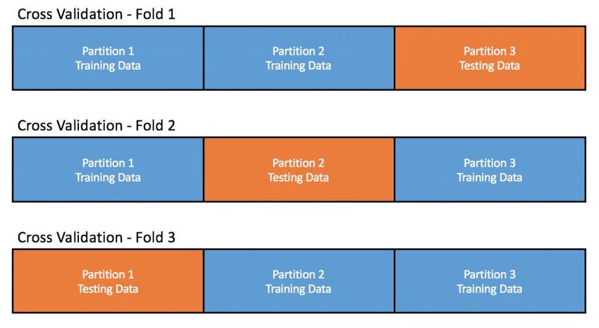
Using supervised learning to predict
English Premier League match results
   from starting line-up player data

                        Student Name
                           Runzuo Yang

A dissertation submitted in partial fulfilment of the requirements of
         Dublin Institute of Technology for the degree of
               MSc. in Computing (Data Analytics)

                               2019

                                 1
I certify that this dissertation which I now submit for examination for the award of MSc
in Computing (Data Analytics), is entirely my own work and has not been taken from
the work of others save and to the extent that such work has been cited and
acknowledged within the test of my work.

This dissertation was prepared according to the regulations for postgraduate study of the
Dublin Institute of Technology and has not been submitted in whole or part for an award
in any other Institute or University.

The work reported on in this dissertation conforms to the principles and requirements of
the Institute’s guidelines for ethics in research.

Signed:         ___________Runzuo Yang______________________

Date:                   03/01/2019

                                              2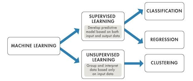
ABSTRACT

Soccer is one of the most popular sports around the world. Many people, whether they
are a fan of a soccer team, a player of online soccer games or even the professional coach
of a soccer team, will attempt to use some relevant data to predict the result of a match.
Many of these kinds of prediction models are built based on data from the match itself,
such as the overall number of shots, yellow or red cards, fouls committed, etc. of the
home and away teams. However, this research attempted to predict soccer game results
(win, draw or loss) based on data from players in the starting line-up during the first 12
weeks of the 2018-2019 season of the English Premier League. It covered their ICT
index, influence, creativity, threat and BPS index, cost and selection by using supervised
Machine Learning techniques, namely Random Forest, Naïve Bayes, K-Nearest
Neighbour and Support Vector Machine. As a result of the research, it was determined
that Random Forest was the best classifier in this project. Influence, creativity, threat,
BPS index and selection were the most suitable features in this model, achieving an
accuracy level of approximately 80%. On this basis, apart from predicting the results,
this model can also provide strategies for coaches, fans and online soccer game players
regarding which kinds of features and positions of players have an essential influence
on the final result, thus affecting how they assign starting line-up.

Key words: Random Forest, Naïve Bayes, K-Nearest Neighbour, Support Vector
Machine, Feature Selection, Players’ data.

                                             3
ACKNOWLEDGEMENTS

First of all, I would like to express my sincere thanks to my supervisor Prof. Sarah Jane
Delany. She is the Head of Postgraduate Studies & Research, School of Computer
Science that has a lot of work and meetings to deal with every day, but she still arranges
a meeting for me every week to guide me carry out the dissertation and patiently answer
my any questions. Let me learn how to logically and critically consider issues and solve
problems, this thinking method not only helps my current dissertation writing but also
affects me in the future study and work. Genuine appreciation from my heart to my
supervisor Prof. Sarah Jane Delany.

Besides, I am also grateful to my initial supervisor Mr. Brian Leahy. Although he cannot
be my supervisor because of his significant increased workload, he still gave me a lot of
inspiration at the beginning of the dissertation.

At the same time, I am thankful for Dr. Luca Longo who is the dissertation coordinator
directed me how to write the dissertation scientifically and rigorously, Mr. Trevor
Conway who helped me fix the mistakes in English proofreading. And all others DIT
tutors and classmates during my postgraduate semesters, they taught me the knowledge
of data analysis and helped me understand this domain better.

Finally, I am going to express my gratitude to my family and friends for comforting and
encouraging me to overcome difficulties when I met problems in study and life.

Thanks to all the people who helped me.

                                             4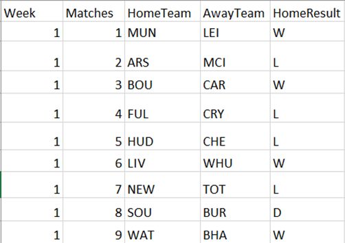
TABLE OF CONTENTS

ABSTRACT ................................................................................................................... 3

ACKNOWLEDGEMENTS............................................................................................ 4

TABLE OF CONTENTS ............................................................................................... 5

TABLE OF FIGURES .................................................................................................... 8

TABLE OF TABLES ................................................................................................... 10

1.      INTRODUCTION ................................................................................................ 12

     1.1 Background ......................................................................................................... 12

     1.2 Research Project ................................................................................................. 13

     1.3 Scope and Limitations ........................................................................................ 13

     1.4 Document Outline............................................................................................... 14

2.      LITERATURE REVIEW AND RELATED WORK ........................................... 15

     2.1 Machine Learning – Algorithms ......................................................................... 16

        2.1.1 Random Forest ............................................................................................. 16

        2.1.2 Support Vector Machine .............................................................................. 17

        2.1.3 Naïve Bayes ................................................................................................. 20

        2.1.4 K-Nearest Neighbour ................................................................................... 21

     2.2 Machine Learning – Feature Selection ............................................................... 21

     2.3 Machine Learning in sports ................................................................................ 21

        2.3.1 Algorithms Comparisons ............................................................................. 22

        2.3.2 Feature selection .......................................................................................... 24

     2.4 Future Development ........................................................................................... 26

3.      DESIGN AND METHODOLOGY ...................................................................... 28

     3.1 Design Outline .................................................................................................... 28

     3.2 Original Data Collection ..................................................................................... 29

     3.3 Data Representation ............................................................................................ 31

                                                               5
3.3.1 One feature for players ................................................................................ 36
3.3.2 Two features for players .............................................................................. 38
3.3.3 Three features for players ............................................................................ 39
3.3.4 Four features for players .............................................................................. 39
3.4 Data Segmentation .............................................................................................. 40
3.4.1 Cross-validation ........................................................................................... 40
3.5 Machine Learning Algorithms ............................................................................ 42
3.6 Feature Selection ................................................................................................ 42
3.7 Evaluation ........................................................................................................... 43
3.7.1 Confusion Matrix ......................................................................................... 43
4. RESULTS, EVALUATION AND DISCUSSION ............................................... 46
4.1 Experiment 1 - Algorithms Comparison............................................................. 46
4.1.1 Random Forest ............................................................................................. 47
4.1.2 Support Vector Machine .............................................................................. 49
4.1.3 Naïve Bayes ................................................................................................. 50
4.1.4 K-Nearest Neighbour ................................................................................... 52
4.1.5 Algorithms Conclusion ................................................................................ 53
4.2 Experiment 2 - Data Size Selection .................................................................... 54
4.3 Experiment 3 - Feature Selection ....................................................................... 56
4.3.1 Experiment 4 – Baseline Feature Selection ................................................. 56
4.3.2 I, C and T with BPS index ........................................................................... 58
4.3.3 I, C and T with Cost..................................................................................... 60
4.3.4 I, C and T with Selection ............................................................................. 60
4.3.5 Conclusion in the first layer ......................................................................... 61
4.3.6 I, C, T, BPS index with Selection ................................................................ 62
4.3.7 I, C, T, BPS index with Cost ....................................................................... 63
4.3.8 Conclusion on the second layer ................................................................... 64
64.3.9 I, C, T, BPS index, Selection with Cost....................................................... 64
4.3.10 Overall Feature Conclusion ....................................................................... 65
4.4 Discussion ........................................................................................................... 66
4.4.1 Matches Analysis ......................................................................................... 66
4.4.2 Players Analysis........................................................................................... 66
4.5 The Latest Prediction .......................................................................................... 69
5. CONCLUSION .................................................................................................... 73
5.1 Research Overview ............................................................................................. 73
5.2 Problem Definition ............................................................................................. 73
5.3 Design/Experimentation, Evaluation & Results ................................................. 73
5.4 Contributions and impact .................................................................................... 74
5.5 Future Work & recommendations ...................................................................... 75
BIBLIOGRAPHY ........................................................................................................ 76
7TABLE OF FIGURES
Fig 2.1 Branches of Machine Learning ........................................................................ 15
Fig 2.2 Processes of Supervised Machine Learning ..................................................... 16
Fig 3.1 The workflow of entire project ......................................................................... 29
Fig 3.2 An example of Starting Line-up in English Premier League ........................... 30
Fig 3.3 An example of a player statistics in English Premier League .......................... 30
Fig 3.4 Features selected from the first source ............................................................. 32
Fig 3.5 Basic constitution of the features in the dataset ............................................... 33
Fig 3.6 Constitution of one feature using ICT index .................................................... 36
Fig 3.7 Constitution of one feature using Influence, Creativity and Threat ................. 37
Fig 3.8 Constitution of one feature using Selection or Cost or BPS index .................. 37
Fig 3.9 Constitution of two features using Baseline with Selection or Cost or BPS index
...................................................................................................................................... 38
Fig 3.10 the principle of 3 folds cross validation ......................................................... 41
Fig 3.11 Distribution of target variable HomeResult .................................................... 41
Fig 3.12 The processes of stratified 3 folds cross validation ........................................ 42
Fig 3.13 The diagram of feature selection .................................................................... 43
Fig 4.1 Summary of normalized data in KNN .............................................................. 52
Fig 4.2 The dataset of one team’s data ......................................................................... 54
Fig 4.3 List of all columns’ name for I, C, T ................................................................ 57
Fig 4.4 List of all columns’ name for I, C, T with BPS index ...................................... 59
Fig 4.5 List of all columns’ name for I, C, T, BPS index with Selection ..................... 62
Fig 4.6 Feature importance of testing fold 3................................................................. 68
Fig 4.7 Feature importance of testing fold 2................................................................. 68
Fig 4.8 Feature importance of testing fold 1................................................................. 69
Fig 4.9 Scatter Plot of the error rate of 216 sub models ............................................... 70
8Fig 4.10 Assessment of the training model .................................................................. 71
Fig 4.11 Confusion Matrix and Statistics of 13th to 15th result ..................................... 71
Fig 4.12 Top 10 importance independent variables from the final result ..................... 72
9TABLE OF TABLES
Table 3.1 All features in official website...................................................................... 31
Table 3.2 Interpretation of BPS index statistics ........................................................... 35
Table 3.3 Interpretation of Confusion Matrix............................................................... 44
Table 4.1 Data distribution and Data segmentation...................................................... 47
Table 4.2 Prediction accuracy and parameters of each test set in RF........................... 48
Table 4.3 Overall confusion matrix for RF with ICT index ......................................... 49
Table 4.4 Prediction accuracy and parameters of each test set in SVM ....................... 49
Table 4.5 Overall confusion matrix for SVM with ICT index ..................................... 50
Table 4.6 Prediction accuracy and parameters of each test set in NB .......................... 51
Table 4.7 Overall confusion matrix for NB with ICT index ........................................ 51
Table 4.8 Prediction accuracy and parameters of each test set in NB .......................... 52
Table 4.9 Overall confusion matrix for KNN with ICT index ..................................... 53
Table 4.10 Prediction accuracy of entire and each class for all classifiers................... 54
Table 4.11 The result of stratified 3 folds cross validation in one team ....................... 55
Table 4.12 Overall confusion matrix of one team’s data.............................................. 55
Table 4.13 Comparison of results of one team’s data and two teams’ data ................. 56
Table 4.14 Prediction accuracy and parameters of each test set in I, C, T ................... 57
Table 4.15 Overall confusion matrix for RF with I, C, T ............................................. 58
Table 4.16 Prediction accuracy comparison between I, C, T and ICT index ............... 58
Table 4.17 Overall confusion matrix for RF with I, C, T and BPS index .................... 60
Table 4.18 Overall confusion matrix for RF with I, C, T and Cost .............................. 60
Table 4.19 Overall confusion matrix for RF with I, C, T and Selection ...................... 61
Table 4.20 Comparison result of the first layer in feature selection ............................. 62
Table 4.21 Overall confusion matrix for RF with I, C, T, BPS index and Selection ... 63
Table 4.22 Overall confusion matrix for RF with I, C, T, BPS index and Cost ........... 63
10Table 4.23 Comparison result of the second layer in feature selection ........................ 64
Table 4.24 Overall confusion matrix for RF with I, C, T, BPS index, Selection with Cost
...................................................................................................................................... 64
Table 4.25 Final results comparison of Feature selection ............................................ 65
Table 4.26 Final confusion matrix after feature selection ............................................ 66
Table 4.27 Data distribution of training data and test data ........................................... 70
111. INTRODUCTION
1.1 Background
Soccer is one of the most popular sports around the world with a significant number of
fans (Razali, Mustapha, Yatim & Ab Aziz, 2017), therefore, predicting the result of each
match is an attractive and exciting thing for audiences to speculate the competitions and
bet respective team. On the other hand, predicting the actual outcomes of soccer games
can also give a series of practical suggestions for the football club to improve their
matches strategies, and has insight into their rivals. The earliest human team activity
with the ball occurred in ancient Mesoamerican cultures over 3000 years, and the
original precursors of soccer game took place in ancient China between the 3rd and 2nd
century BC1. However, the beginning of the modern soccer was in England in 18632.
Nowadays, the English Premier League is the top level of English soccer organization
and one of the most powerful leagues in the international soccer field. Each team in this
league has the same chance to win the final championship. A top team may occasionally
fail to win a match when it competes against a weak team. Different teams will arrange
diverse starting line-up against various types of opponents. This research will focus on
the statistics of players in the starting line-up in each match over a certain period, and it
will use these features to build a series of models, predicting match results by using
supervised Machine Learning techniques.
There are many algorithms in Machine Learning that have been applied to the prediction
of sports especially soccer competitions. Bayesian Network is an appropriate method to
build and develop predicting models in soccer games (Zhao & Xie, 2015). As a
consequence of the dataset, it has a series of sophisticated features with quite small
sample sizes, handling missing values and avoiding overfitting issues (Uusitalo, L.
2007). Naïve Bayes which is another approach based on the Bayesian theorem that is
commonly used in classification cases, and it can calculate the distribution of each class
in target variable (Hai, M., Zhang, Y., & Zhang, Y. 2017). Moreover, the K-nearest
neighbours’ algorithm, Random forest, LogitBoost, and Artificial neural networks also
applied to achieve and compare the accuracy of prediction results in soccer games
(Hucaljuk, J. & Rakipović, A. 2011). In order to discuss the performance of feature
selection and variables’ correlation coefficient, regression models can also be taken
1
https://www.footballhistory.org/
2
https://www.fifa.com/about-fifa/who-we-are/the-game/
12advantage of predicting Australian football which is similar to British soccer (Jelinek,
Kelarev, Robinson, Stranieri & Cornforth, 2014).
1.2 Research Project
This research aims to predict matches results based on data from players in the starting
line-up of the English Premier League by using supervised Machine Learning techniques.
As a result of that, the research question as follows:
“Can people use the data of players in starting line-up to predict soccer game results by
using supervised Machine Learning techniques?”
The data for this the research was collected from the first 12 match weeks of the
2018/2019 season of the English Premier League, involving a total of 120 games (10
matches each week). Information regarding home and away teams’ names, starting line-
up lists and final results were acquired from https://www.premierleague.com/results.
The personal data of the players was obtained from https://fantasy.premierleague.com/.
The research will choose the classifier with the highest prediction accuracy to build the
training model from Random Forest, Support Vector Machine, Naïve Bayes and Nearest
Neighbour. Subsequently, it will use this classifier for feature selection to select the most
appropriate features. Eventually, the model will evaluate and analyse the prediction
results and summarise the importance of various features of players in different positions.
As a result, the final model can provide suggestions and solutions for online players or
fans, and even professional coaches.
1.3 Scope and Limitations
This research was completed based on data from the first 12 weeks of the Premier
League 2018-2019 season. Due to the limited size of the dataset, it can only be used for
the current season; this model cannot be applied to other seasons. Furthermore, this
project mainly used the starting line-up, so the performance of substitute players and the
changing dynamics of starting players’ positions were not reflected. To test the
feasibility and stability of this project, an extra experiment was applied to predict the
results from the 13th to the 15th weeks, based on the previous 12 weeks, because the
season is not over yet, and the 13th to 15th weeks included the latest matches at the time
of writing.
131.4 Document Outline
This research is organised as follows.
Chapter 2 discusses, compares and summarises various literature which used different
Machine Learning techniques to predict the results of soccer games, determining their
advantages and disadvantages. It also explains the methodologies of the Machine
Learning techniques, along with the feature selection used in this project.
Chapter 3 concentrates on the general structure of this prediction system, regarding
which kinds of techniques should be used and the methodologies adopted for each step,
from data selection to model evaluation.
Chapter 4 describes each model used for each experiment in this project in a step-by-
step fashion, interpreting their modelling, parameter-fixing and predicting processes.
Evaluating and analysing the results and findings from this series of experiments.
Chapter 5 aims to give a general review of the entire project. It discusses the final result
and conclusion, highlighting the limitations and problems relating to this project, and it
gives suggestions for future work in the effort to improve research in this field.
142. LITERATURE REVIEW AND RELATED WORK
In this chapter, several fields of literature will be listed and be discussed, covering
Machine Learning algorithms, datasets, features, etc., to compare and conclude their
study results or findings. This will be done to find suggestions and inspirations from
previous work to improve the prediction accuracy of soccer matches’ results for this
project. In addition, this chapter will be divided into two parts. Part one is from Section
2.1 to Section 2.2 which focuses on the methodology of Machine Learning algorithms,
feature selection. This part describes the principles of Machine Learning algorithms and
related work and how they will be used in this project. Part two is from Section 2.3 to
Section 2.4 which reviews how other researchers apply Machine Learning techniques
and select or collect data sets for prediction in the field of sports, especially in soccer
games.
Fig 2.1 Branches of Machine Learning
As Fig 2.1 shows, Machine Learning is classified as supervised and unsupervised
learning. The sports industry always belongs to the former one, because people can
acquire both input and output information frequently. As a result, people may develop
an available model to attempt to predict the outcome for the next time. Besides, this
project will use supervisory classification to predict results because of the existence of
a categorical target variable. The basic processes are as Fig 2.2 illustrates:
15Fig 2.2 Processes of Supervised Machine Learning
Firstly, the Machine Learning model acquires labelled observations from the raw data
source and then adjusts the quality of them and after that the system divides them into
the training set and test set selecting suitable Machine Learning algorithms to build the
prediction model based on the training set. The label of observations should be removed
in the test set. Finally, the experiment will predict the results by using the training model,
comparing the result with the label-removed test set and calculating prediction accuracy
afterward.
After a brief explanation of the workflow of supervised Machine Learning, the next
Section 2.1 (from Section 2.1.1 to Section 2.1.4) is going to describe four kinds of
favourite Machine Learning algorithms which frequently appear in the literature to be
discussed, and a Machine Learning feature selection in Section 2.2 which is an essential
step in the entire Machine Learning process.
2.1 Machine Learning – Algorithms
The following subsections are going to introduce four supervised Machine Learning
algorithms which will be applied in Chapter 4.
2.1.1 Random Forest
Random forest is an ensemble Machine Learning method for classification by using the
decision tree as a basic learner device to build bagging and further introduces random
attributes in the training process of the decision tree. The algorithm procedures are:
(1) Assume that there is a data set that has N
number of features, the samples under bootstrap sample can generate
sampling space
16(2) Building a base learner (decision tree): sampling each one like
(k should be less than m) to generate the
decision tree and record each result of it as
(3) Training T times let in the formula that
which is a kind of decision algorithm (includes absolute majority voting,
plurality voting, and weighted voting, etc.)
In (1) and (2) steps, the input samples in each tree will not include the whole sample,
and each decision tree is established in a completely split manner, so that one leaf node
of the decision tree cannot continue to split, or all the samples in the same class are
directed to the same classification. Both of them ensure the randomness of sampling
which does not need to prune the branches and can avoid the problem of overfitting
problem.
Random forest does not need to adjust too many parameters compared with other
machine semester algorithms. Baboota & Kaur (2018) summarized that the most
parameters that needed to be optimized for their random forest model were the number
of trees to build, the splitting criterion to consider, the maximum depth of each tree and
the minimum sample split. Ulmer & Fernandez (2014) tuned the number of estimators
and minimum sample required to split an internal node by using the grid search,
acquiring the third lowest error rates in their models’ comparison.
2.1.2 Support Vector Machine
Baboota & Kaur (2018) provided a brief explanation for non-linear classification in the
Support Vector Machine. SVMs have an excellent performance in dealing with high-
dimensional feature spaces, because, through some pre-selected non-linear mapping
(kernels trick), this transforms it into a linear separable dimension in a high-dimensional
space, and constructs an optimal classification hyperplane in this high-dimensional
space. The formula of non-linear SVM is as follows Equation 2.1:
Equation 2.1
17The mapping of φ from the input space (X) to a specific feature space (F) means that the
establishment of a non-linear learner is divided into two steps: The first step is
transforming the data into a feature space F using a nonlinear map. Then the second one
is using the linear learner classification in the feature space.
Kernel is a way to calculate the inner product directly in the feature
space and combine the above two steps to build a linear learner. In a word, Kernel is
like a function K, for all , it should be satisfied with
and φ (·) has the same meaning as φ in the non-linear SVM. Calling a method of
replacing an inner product with a kernel function is named kernel trick. Baboota and
Kaur selected the radial basis kernel and the linear kernel in their project tuned the two
main hyper-parameters for SVM models which are C and Gamma. The C is the cost of
misclassification on the training data, the lower value represents a smooth decision
surface. In contrast, the higher value shows that the model needs more cases to support
vectors to classify all training cases correctly (Ancona, Cicirelli, Branca & Distante,
2001). Consequently, a suitable C should keep a balance between under-fitting and over-
fitting. Gramma comes from the Gaussian radial basis function: a higher Gamma will
lead to a small variance and a high bias that reflects the support vector’s lack of extensive
influence.
This project is going to develop a comparison function in R language which is used to
select the least error rate of four common kinds of kernels function. Except for the two
types which were mentioned in the previous ,there are
Polynomial kernel and Sigmoid kernel as well, the Polynomial kernel is non-fixed
kernels, and it is ideal for normalizing all training data, which calculate formula as
follows: generally, it is not appropriate to choose a high dimension.
The most suitable dimension needs to be selected by cross-validation. The Sigmoid
kernel function is calculated as follows: which is a common S-type function derived
from neural networks and now heavily used for deep learning. When there is a kernel
trick, the support vector machine implements a multi-layer perceptron neural network,
applying the SVM method, the number of hidden layer nodes (which determines the
structure of the neural network), and the weight of the hidden layer nodes to the input
nodes. Values are automatically determined during the design (training) process.
Moreover, the theoretical basis of the support vector machine determines that it finally
obtains the optimal global value rather than the local minimum, and also guarantees its
18good generalization ability for unknown samples without over-learning. Apart from
that, as the precondition of modelling, the dataset should be normalized so that all of the
value should fall in between 0 to 1.
So far, this part has discussed how to deal with independent variables in SVM, and this
paragraph will interpret the dependent variable in this dataset. The SVM algorithm was
initially designed for the binary classification problem. When dealing with multiple
types of issues, it is necessary to construct a suitable multi-class classifier. At present,
there are two main methods for creating SVM multi-class classifiers. (1) The direct
method, directly modifies the objective function, merge the parameter solutions of
multiple classification surfaces into one optimization problem, and realize multi-class
classification by solving the optimization problem “one-time”. This method seems
simple, but its computational complexity is relatively high, and it is difficult to
implement. It is only suitable for small problems. (2) The indirect method mainly
performs the construction of a multi-classifier by combining a plurality of two
classifiers, and the conventional techniques are one against one and one against all. In
the training step of one against one, the samples of a particular category are classified
into one class, and the other remaining samples are classified into another class, so that
the samples of the K categories construct K SVMs. When classifying, the unknown
sample is classified as the one with the most substantial classification function value.
However, this method has a drawback because the training set is 1: M that always
produce quite obviously biased data in the other classifier with remaining samples. The
second approach is to design an SVM between any two types of samples, so K samples
need to develop K(K-1)/2 SVMs, when an unknown sample is classified, the category
with the most votes last is the category of the target. In this project, the target variable
has three kinds of classifications (W, L, and D). The process by using one against all is:
In the beginning assume that W=L=D=0. Selecting W and L to build the model, if W
has a higher prediction accuracy, W win the comparison and W=W+1, otherwise,
L=L+1. Selecting W and D to build the model, if W has a higher prediction accuracy,
A win the comparison and W=W+1, otherwise, D=D+1. Selecting D and L to build the
model, if D has a higher prediction accuracy, D wins the comparison and D=D+1,
otherwise, L=L+1. The final result is the Max(W, L, D). Because there are only three
categories in the project, it only builds 3(3-1)/2 = 3 SVMs, in the end, one against all
will be applied in these multiple SVM models.
192.1.3 Naïve Bayes
Naive Bayes classification uses a probabilistic classifier to predict maximum likelihood-
based results. The model assumes that all variables in the dataset used to predict the
target value are independent. The classification model is based on the assumption that
the value of a feature in the dataset does not depend on the values of other features in
the dataset. It focuses on the dependent variable and then thinks over the probability of
the given value that independent variables have, determining which one has the highest
probability. The dependent variable will fall in that classification (Hijmans & Bhulai,
2017).
The basic theory of the Naive Bayesian classification is as follows:
(1) Firstly, selecting a known classification of items to be classified as training samples
and assume that the category set of the sample is represented as
Sample has n discrete features, expressed as: any
is the feature attribute of the sample.
(2) Secondly, calculating separately
If any individual in the training sample is satisfied with the following
formula:
it can be regarded as and then according to the Bayes’ theorem Equation
2.2:
Equation 2.2
to calculate the conditional probability of each category of the sample. Because the
denominator is the same value for all categories, it can be omitted. Whichever, one has
the highest numerator that is the suitable class for the target variable. Although the
assumption that "all features are independent of each other" is unlikely to be right in
reality, it can significantly simplify the calculations, and studies have shown that the
accuracy of the classification results has little effect.
202.1.4 K-Nearest Neighbour
Hucaljuk & Rakipović (2011) illustrated that the K-nearest neighbour is the
representative algorithm of lazy classifiers which classifies a new example by finding
the k nearest neighbours in the space of features such as the Euclidean distance
measurement from others examples in the existing learning set. After that, based on the
learning set, to make a vote determines the classification of the unknown case. The
concept as described is to find the appropriate K value and how to select the calculation
methods are essential steps in the K-nearest neighbour.
2.2 Machine Learning – Feature Selection
The goal of feature selection is to maximize the extraction of features from raw data for
use by Machine Learning algorithms and models. According to the form of feature
selection, there are three popular methods nowadays:
Filter: The Filter method, which scores each feature according to divergence or
correlation, sets the threshold or the number of thresholds to be selected, and selects
features.
Wrapper: A wrapper method that selects several features at a time, or excludes several
features, based on an objective function (usually a predictive effect score).
Embedded: The embedding method, which first uses some Machine Learning algorithms
and models to train, obtains the weight coefficients of each feature and selects features
according to the coefficients from the large value to the small value. It is similar to the
Filter method, but it is trained to determine the pros and cons of the feature.
When comparing the first two methods, the filtering method does not consider the effect
of the feature on the learner when selecting features, but the wrapped selection is more
flexible. Parcels are usually “tailor-made” feature subsets for learners based on
predictive performance scores. Compared with filtering methods, learners can perform
better. The disadvantage is that the computational overhead is often higher.
2.3 Machine Learning in sports
Machine Learning algorithms are more and more widely and frequently used in
competitive sports. They use historical records, as well as live real-time game data, to
build models that predict what might happen in the future. Some studies have proved
that the application of Machine Learning in sports has established a systematic approach
21and has achieved quite good results and experience. The following sections are the
guided review of these kinds of literature.
2.3.1 Algorithms Comparisons
In this section, the literature review will mainly focus on the Machine Learning
algorithms used in several sports, but the majority materials are only relevant to soccer
matches and describe their dataset and features as well.
Soccer matches are one of the most popular branches of sport prediction. There are other
kinds of ball games which are similar to soccer that are referred to in this research. Delen,
Cogdell & Kasap (2012) predicted the NCAA bowl outcomes by using artificial neural
networks, decision trees and support vector machines based on eight seasons’ data and
36 variables. Continuous variables are inputted from the home team’s perspective by
calculating and using the different values between home and away teams. Their scenario
is building and comparing the direct classification and regression-based classification
models which output both wins and losses. Finally, decision trees which represent the
direct classification method got better than an 85% prediction accuracy that defeated the
other one. Leung & Joseph, (2014) attempted to predict the same target as Delen,
Cogdell and Kasap, however, they explored the results of similar level teams, using their
data to predict the result of this team with the same opponent instead of comparing these
two teams directly. Leung and Joseph made the model compared with the exciting
models from previous researches they referenced and even got 97.14% accuracy, this
high accuracy may be because of a potential multicollinearity problem during the feature
selection step, considering more reliable reference models could also be adopted in
further work.
Returning to the soccer domain Min, Kim, Choe, Eom & (Bob) McKay (2008) proposed
a Football Result Expert System (FRES) which predicted the soccer result based on a
multiple framework composed by Bayesian networks and a rule-based reasoner.
Owramipur, Eskandarian & Mozneb (2013) applied a similar construction to predict the
result of Spanish League match involving Barcelona as well. The features classification
is different from Min, Kim, Choe, Eom & (Bob) McKay (2008) in that their variables
are divided into psychological data such as weather, historical records, psychological
condition, etc. and non-psychological data such as the average age of players, average
goals in each match, average matches each week, etc. The FRES can give a somewhat
22steady and reliable output between two clubs which was seldom encountered in previous
matches. The authors mentioned that the Bayesian models are good at merging uncertain
human knowledge and probative knowledge. However, their construction of the
knowledge is inclined to a subject activity. It cannot be applied without expert
knowledge, and this is a common limitation in a knowledge-based system. FRES by
from coach’s perspective, organizing Bayesian networks for offense, defence,
possession and fatigue strategies, generating optimum discrete values from each section
and passing to the rule-based reasoner to adjust the initial output and carry out entire
appropriate strategies. Bayesian networks and other technologies can also operate the
parameter learning to tune each position’s output automatically, combine it with the rule-
based reasoner to establish the fundamental team knowledge probably producing a more
reasonable strategy for the football team.
Hijmans & Bhulai (2017) worked on predicting Dutch football by using Machine
Learning classifiers along with random forest, Naïve Bayes and the k-nearest neighbour
models. Their work had an interesting result, finding that the tactics of the team coach
do not have much effect on the final result of a match. The dataset is composed of three
types of matches which are friendly, qualification and tournament, with the details of
individual players adopted in it as well. In the random forest models, the authors applied
the generalized boost method, which can synthetically use weak predictors and generate
a series of constraints for each node of decision trees to control the random outputs or
overfitting issues, testing different nodes to find out the best fit tree. The prerequisites
for Naïve Bayes are that one variable will not depend on other variables in the same
dataset. The case will be applied to whichever class has the highest probability. For
instance, the following Equation 2.3 is acquired from the model:
Win = P(win)*P(age|win) *P(attrackers|win) *P(home|win) / normalization constant
Equation 2.3
In this research, the authors chose to use the maximum or minimum value replacing the
outliers during the data cleaning stage instead of using the average value, as this might
influence the final accuracy and methods selection of experiments.
The Bayesian networks models are frequently mentioned in research studies. Joseph,
Fenton & Neil (2006) used and compared expert Bayesian networks, MC4 (which
23identifies factors with the most significant effect on the match result), k-nearest
neighbour, Naïve Bayes and Data-Driven Bayesian (which entirely learns from the
dataset) to predict soccer results. They focused on Tottenham Hotspur Football Club and
used 1995 to 1997 season’s data to constitute the dataset which is the first time to
develop the expert Bayesian networks in the English Premier League, so it was an
uncommon opportunity for making a comparison between expert Bayesian networks
models and others Machine Learning models directly. It is a distinctive point, but it also
means the dataset is probably quite old and rare at the same time. The expert BN picked
some key pieces of information from several core players as the fundamental parameters.
Others used more players’ information (position, attendance, and performance) as a
result of the experiment, with the complete two seasons as the dataset KNN got the best
performance when disjoint training and test data, the expert BN won the competition.
However, the biggest disadvantaged of the expert BN model is that players might change
their position or even change their football club in their career. Hence it cannot provide
a sustainable use for a long time. Besides, expanding data from other teams in the league
could help to construct more symmetrical models for Bayesian networks to strengthen
their accuracy and stability (their results are in the range of 38% to 59% so far).
96% is one of the highest average prediction accuracies found in one research study by
(Martins et al., 2017). Their dataset was collected from different soccer leagues with
different seasons, such as England, Spain, and Brazil, from 2010 to 2015. They
introduced a polynomial classifier which used polynomial algorithms to expand input
data in an advanced dimension and separate analysed classes and output as nonlinear
data. Making a comparison between the support vector machine, Naïve Bayes and
decision trees, it costs more time than others to dispose of dimensionality problems with
multiple features, due to the complicated procedures; consequently, this system is not
suitable to be used in real-time prediction at present.
2.3.2 Feature selection
Feature selection is the primary and initial step for a Machine Learning model which
affects the decision of project objectives and the quality of models’ results. As
mentioned in the previous section 2.3.1, Joseph, Fenton & Neil (2006) used players’
data from the Tottenham Hotspur football club, but other researchers prefer to select the
data from matches themselves. However, all the statistics during the matches are made
by each player. This project and the following researchers that will now be discussed
24chose a different aspect of the dataset and features based on information of players to
explore more interesting or useful performances.
Pariath, Shah, Surve & Mittal (2018) considered their system from the perspective of
coaches and team management, estimated and generated a performance value for one
soccer player from his value budget, competitiveness, position and skills in his
individual career. As a result of that, they scrapped data which included 21280 players
with 36 attributes from the grassroots level of players in India from the 2017 version of
EA sports. The overall performance accuracy can reach 84.34%, and market value
prediction accuracy is around 91% under the linear regression model. During the
modelling step, Pariath, Shah, Surve & Mittal tried to separate players in a different
position (Forward, Midfielder, Defender and Goalkeeper) which provided a balanced
exploration for players in their proper and individual standard.
Some researchers mainly concentrated on English Premier League research. Their
datasets ranged approximately from 2006-2007 to 2012-2013 seasons. Bush, Barnes,
Archer, Hogg & Bradley (2015) investigated specific position evolution of players and
generated relevant parameters, to evaluate match performance, their project can also
simulate the view of coach to arrange the squads. The Genetic Programming system
which produced a series of GP-generated functions according to different parameters,
weights, and settings, followed a majority voting method that combined superior quality
functions to get better prediction (Cui, Li, Woodward & Parkes, 2013). Archer, Hogg &
Bradley (2015) combined 43 GP-generated functions and got an average predicting
accuracy around of 75% eventually which had a more excellent performance than
ANN’s result.
McHale & Relton (2018) identified the key players in soccer teams by using network
analysis and pass difficulty. They acquired professional datasets from Prozone which is
a company dedicates sports data and related technologies. The dataset includes 380
matches with the tracking data of players covering passes, tackles, dribbles, and shots,
etc. in 2012 to 2013 season for English Premier League. The pass difficulty is defined
as the probability of the successful pass by using a weighting scheme which can identify
who has the highest threat to get a score for the attacking team. McHale & Relton also
examined more positions than others researchers. The goalkeeper, central back, full back,
wide midfield, central midfield and attacker in their model which is much closer to the
25actual matches. However, this research mainly considered the total distance and the total
number of sprints by each team as the target which cannot represent diverse strategies
in the English Premier League, and different scores during the match will lead and
change their running distance and sprints in the particular period.
Sarangi & Unlu (2010) conducted a similar study to McHale & Relton’s (2018), where
they collected data from the UEFA Euro 2008 Tournament and explored how the players’
contribution affected their team and their salaries, constructed a team network analysis
based on individual actions and interactions between players. Passing and receiving are
important indexes in helping to calculate the team’s intercentrality measure which is
regarded as the final team performance index. As a result, the key player in a team is
always the person who keeps the most frequent interaction with teammates, not the
person who has the maximum kicks at goal. Sarangi & Unlu did not divide players into
their specific position as it was not suitable for the exploration of the team line-up during
a match. Using defensive data like tackling and dribbling data will more scientific to
assess the strong probability of interaction between players.
2.4 Future Development
There are also some new and unique ideas that can be applied in future design and
improvement for this project which have been successful modelling cases as described
in the following paragraphs.
Lu, Chen, Little & He (2018) carried out their project from a different kind of dataset.
They extracted information from images and videos of different sports which consist of
soccer, basketball, ice hockey. They used the convolutional neural network (CNN) to
classify and predict team memberships for both teams or specific positions in the line-
up on the field, which can be developed in the future and more profound experiments
for this graduation project.
On the match field, not only are there 22 players from the home and away teams but also
have professional referees. Most researchers will not select the data from the statistic of
referees to predict matches results, which might be a new field for further exploration.
Weston, Castagna, Impellizzeri, Rampinini & Abt (2007) proposed three variables: 1)
total distance covered, 2) high-intensity running distance whose running speed more
than 5.5m/s and 3) average distance from infringements will influence the physical
performance of referees and tactical strategies on behalf of the referees, even the tempo
26of match. Weston, Bird, Helsen, Nevill & Castagna (2006) also illustrated the second
half match time would change the standard of judgment and intensity of competition.
All of these factors have the potential to decide the matches’ result.
This chapter described in detail the technical principles involved in this research and the
application of Machine Learning in sports competitions, especially soccer games in the
literature review. The following chapter will introduce the design and process details of
the prediction model.
273. DESIGN AND METHODOLOGY
In the third chapter, the research will discuss the general process of how to use players’
data in the starting line-up to predict the result in English Premier League. The model
describes details of original data, for instance, the reason why the project selected the
dataset, how to pre-process different features in the entire dataset, and explain the
meaning of each feature.
3.1 Design Outline
Both Chapters 3 and 4 will develop their work according to the design outline as
following Fig 3.1:
(1) Data collection - Describe the data source and features meaning from perspectives
of both matches and players in Chapter 3.
(2) Data construction - Explain the structure of datasets (from 1 to 4 features for players)
and demonstrate the data segmentation in Chapter 3.
(3) Cross validation – Interpret its operating principle in Chapter 3. Use this method to
divide the training set and test set in order to get the most reliable and stable model in
Chapter 4.
(4) Algorithms comparison - Illustrate individual parameters for tuning for each
algorithm and select the best classifier for feature selection in Chapter 4.
(5) Feature selection - Describe the methodology of feature selection in Chapter 3. Select
the excellent features which can generate the highest prediction accuracy in Chapter 4.
(6) Final Model - After determining the final model, two kinds of analysis include
matches and players will be provided for people as a reference.
28Fig 3.1 The workflow of entire project
3.2 Original Data Collection
The entire dataset consists of two sources which are the introduction of each match and
the statistics of players in the starting line-up each match. The first source is a CSV
format document for match results in the English Premier League which are collected
from: https://www.premierleague.com/results. This is the official website of the English
Premier League which provides the latest and specific statistics for each match in each
week. There are 20 teams in the English Premier League and 10 matches for each week.
As a result of that, this project decided to import the last 12 weeks’ matches (totalling
120 matches) of the English Premier League in the 2018/2019 season when this
dissertation start to write on October,2018. The entire data will be imported in the further
experiments until this season is completed. The other reason why this project only uses
120 matches for the current season is that the soccer market keeps a high dynamic
situation. A team cannot ensure that one player will still be playing for the same football
club after the transfer period in the summer or winter and so the tactical arrangements
for starting line-up might be quite distinctive under different coaches and seasons. This
project extracts 120 matches with their match weeks, names of home teams and away
teams, match results, goals of home teams and away teams. Besides, the starting line-up
list of the match is also provided in the sub-link of this link, click on the result of each
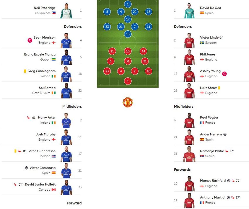
match to acquire the specific information which the following Fig 3.2 demonstrates.
29Fig 3.2 An example of Starting Line-up in English Premier League
The second source is the statistics of players in the starting line-up which is typed
manually into an XLSX format document which is built based on
https://fantasy.premierleague.com/, the following Fig 3.3 is an example of the data
source of a player. The statistical table involves the player’s name, his position and
football club and relevant features in each match of this season.
Fig 3.3 An example of a player’s statistics in the English Premier League
30You can also read