ESTIMATING SATELLITE-DERIVED BATHYMETRY (SDB) WITH THE GOOGLE EARTH ENGINE AND SENTINEL-2 - PUMA
←
→
Page content transcription
If your browser does not render page correctly, please read the page content below
remote sensing
Technical Note
Estimating Satellite-Derived Bathymetry (SDB) with
the Google Earth Engine and Sentinel-2
Dimosthenis Traganos 1 ID , Dimitris Poursanidis 2, *    ID
                                                              , Bharat Aggarwal 1 ,
Nektarios Chrysoulakis 2 ID and Peter Reinartz 3 ID
 1   German Aerospace Center (DLR), Remote Sensing Technology Institute, Rutherfordstraße 2,
     12489 Berlin, Germany; Dimosthenis.Traganos@dlr.de (D.T.); 851.bharat@gmail.com (B.A.)
 2   Foundation for Research and Technology—Hellas (FORTH), Institute of Applied and Computational
     Mathematics, N. Plastira 100, Vassilika Vouton, 70013 Heraklion, Greece; zedd2@iacm.forth.gr
 3   German Aerospace Center (DLR), Earth Observation Center (EOC), 82234 Weßling, Germany;
     peter.reinartz@dlr.de
 *   Correspondence: dpoursanidis@iacm.forth.gr, Tel.: +30-2810-391774

 Received: 7 May 2018; Accepted: 30 May 2018; Published: 1 June 2018

 Abstract: Bathymetry mapping forms the basis of understanding physical, economic, and ecological
 processes in the vastly biodiverse coastal fringes of our planet which are subjected to constant
 anthropogenic pressure. Here, we pair recent advances in cloud computing using the geospatial
 platform of the Google Earth Engine (GEE) with optical remote sensing technology using the open
 Sentinel-2 archive, obtaining low-cost in situ collected data to develop an empirical preprocessing
 workflow for estimating satellite-derived bathymetry (SDB). The workflow implements widely
 used and well-established algorithms, including cloud, atmospheric, and sun glint corrections,
 image composition and radiometric normalisation to address intra- and inter-image interferences
 before training, and validation of four SDB algorithms in three sites of the Aegean Sea in
 the Eastern Mediterranean. Best accuracy values for training and validation were R2 = 0.79,
 RMSE = 1.39 m, and R2 = 0.9, RMSE = 1.67 m, respectively. The increased accuracy highlights the
 importance of the radiometric normalisation given spatially independent calibration and validation
 datasets. Spatial error maps reveal over-prediction over low-reflectance and very shallow seabeds,
 and under-prediction over high-reflectance (17 m). We provide
 access to the developed code, allowing users to map bathymetry by customising the time range based
 on the field data acquisition dates and the optical conditions of their study area.

 Keywords: satellite-derived bathymetry; image composition; pseudo-invariant features; sun glint
 correction; empirical; spatial error; Google Earth Engine; low cost in situ; Sentinel-2; Mediterranean

1. Introduction
     Bathymetry is important for understanding how global Earth processes interact as they influence
the flow of the sea water carrying heat, salt, nutrients, and pollutants. Bathymetry also aids in
understanding the propagation of energy from undersea seismic events that impact navigation and
commerce, and shape habitats for marine life, especially in coastal areas [1,2]. Coastal areas are
under constant pressure due to intense anthropogenic activities such as urbanisation, exploitation of
natural resources, and climate change-induced natural hazards (e.g., coastal erosion due to sea level
changes) [1]. The littoral zone of this interface is spatially complex and determines biodiversity-related
processes as increasing bathymetric values decrease light penetration and cause changes in habitat
compositions and the depth zonation of biota [2]. Studies of the coastal zone—including the modelling
of tsunami expansion and wave height estimations, sea-level change scenarios, risk assessment,

Remote Sens. 2018, 10, 859; doi:10.3390/rs10060859                        www.mdpi.com/journal/remotesensing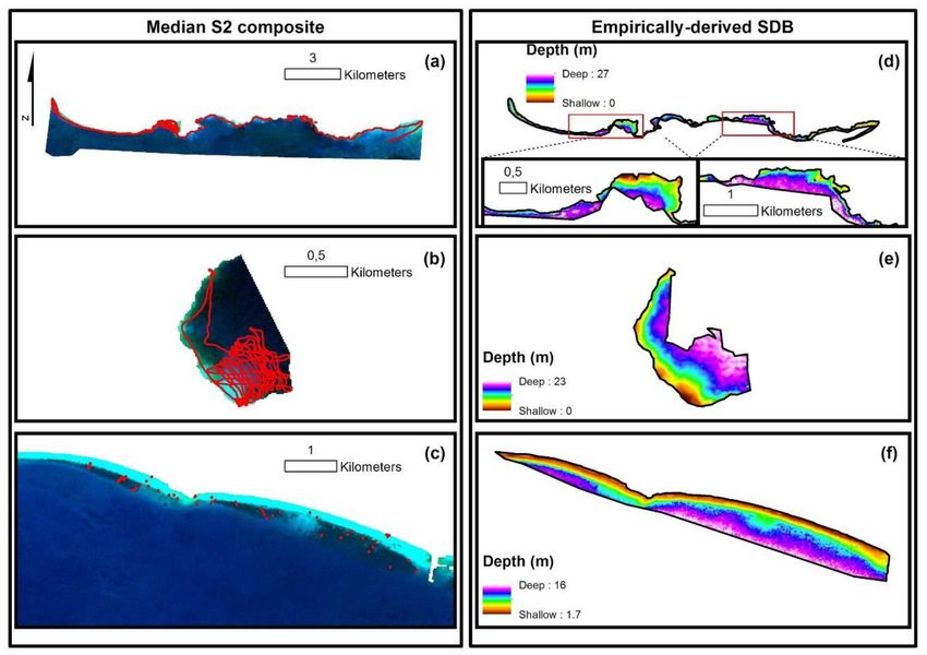
Remote Sens. 2018, 10, 859                                                                          2 of 18

and coastal habitat mapping—require the availability or the creation of updated bathymetric data of
high (10 m) to very high resolution (2 m) [3–6]. Up to today, numerous researchers have mapped
coastal bathymetry with a range of different tools and methods of variable spatial and temporal
resolution, but with increased cost. Globally, bathymetry has been extracted by the inversion of
the spaceborne geoid data from Geosat and the European Remote Sensing satellite ERS-1 [7] at
12-km spatial resolution as well as from a combination of sound navigation and ranging (SONAR)
multibeam sounding data from marine agencies and an improved gravity model from CryoSat-2
and Jason-1 at a 500-m resolution [8]. With respect to currently open access data, Landsat missions,
especially Landsat 8 Operational Land Imager (OLI) due to the availability of its coastal/aerosol
band 1 centred at a 443-nm wavelength featuring high water penetration) open a new window in
coastal satellite-derived bathymetry (SDB) due to their spatial (30-m) and temporal (16-day) resolution.
With these characteristics, the Landsat program allows for the selection of proper images (cloud-free
or atmospheric images, surface and water column conditions) and the testing of hypertemporal
approaches for monitoring changes in seabed morphology [9–11]. The more recently launched
Copernicus Sentinel-2 twin-satellite mission has created a new era in terrestrial and marine monitoring
due to its high spatial resolution of 10 m, availability of a coastal/aerosol band at 443 nm (60-m spatial
resolution), quick revisit time of 5 days, and more significantly, its open and free data access policy.
Focusing on SDB, studies have employed Sentinel-2 data in shallow inland waters [12] and semi-closed
bays [13,14] with promising results, but not at large scales, with notable differences in the water
column and seabed composition. The aforementioned optical sensor technology, machine learning
algorithms, and cloud computing system infrastructures provide an unprecedented environment for
high spatiotemporal large-scale analysis of natural and anthropogenic ecosystems and associated
biophysical variables. Among the available cloud systems, Google Earth Engine (GEE) [15] has
attracted the attention of environmental scientists due to its unique components. GEE is a cloud-based
geospatial computing platform which offers a petabyte-scale archive of freely available optical satellite
imagery. Among characteristics, it features the whole archive of Landsat, the first three Sentinel
missions, and full Moderate Resolution Imaging Spectroradiometer (MODIS) data and products.
Researchers have utilised it for country-scale vegetation metrics [16], continental-scale mapping of
croplands [17], and global land surface temperature [18] and albedo [19] estimation.
      Here, we have developed an empirical preprocessing workflow within GEE to estimate four
satellite-derived bathymetry algorithms using Sentinel-2 images at three different locations in the
Eastern Mediterranean. The preprocessing chain of Sentinel-2 data combines a plethora of simple,
widely used, and well-established cloud, atmospheric, and sun glint corrections with a seasonal 10-m
image composition approach (median composites). The latter approach opts to reduce the effects of
variable water surface conditions, water quality, and related optical properties such as sun glint and sky
glint, whitecaps, turbidity, and sedimentation etc. Furthermore, we implement in situ data acquired by
a low-cost methodology in the training and validation of the SDB which shows, in turn, promising
results for a time- and cost-efficient epoch for wide-scale SDB. We perform the training and validation
of the four empirical models in different optically shallow environments to reduce the statistical bias
according to the first law of geography by Tobler [20]—spatially neighbouring observations tend to
be more similar than the ones further apart. Moreover, we employ a pseudo-invariant-feature (PIF)
approach to normalise the differences in the reflectance ranges between the pre-processed composites
used in the training and validation steps [21]. Finally, we map the model residuals of the SDB maps
to unveil possible over- or under-prediction patterns. Our proposed method can be widely adapted
in a cloud computing environment for estimating large-scale coastal bathymetry given, naturally,
the availability of relevant open access in situ data.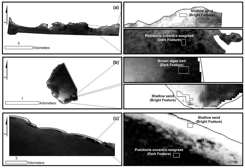
Remote Sens. 2018, 10, 859 3 of 18
2. Materials and Methods
2.1. Study Sites and In Situ Data
Figure 1 shows our three study sites; the first study site is Samaria National Park in the southern
part of West Crete, Greece, in the Eastern Mediterranean. The selected area covers the east part of the
National Park. Mixed habitats cover the seabed here, while depths vary from smooth areas to steep
ridges and provide a challenging seascape for space-borne coastal bathymetry. Seagrass meadows
reach depths of 40 meters [22]. Bathymetric data was collected during the period 2012–2015 by means
of a 5-m inflatable boat using a Lowrance High Definition System (HDS)-5 single-beam echosounder
with the HST-WSU 83/200 kHz Skimmer Transducer. The Global Positioning System (GPS) was
positioned on top of the roll bar, directly above the transducer to record the exact position. Data was
recorded with a frequency of 1 Hz. Preprocessing of Lowrance files was performed using DrDepth
software. Data was imported in ArcMap 10.5 in comma separated value (CSV) format and converted
into a three-dimensional shapefile for further use. The second study site is Apokoronas area (Obros
Gyalos) in West Crete, close to Georgioupolis Bay. It is a remote area with a mixed bottom—shallow
rocky reefs followed by bright white sand substrate, ending with seagrass meadows which are followed
by a mixed pebble/sand substrate. In this location, the first diving park in Crete is under development,
acting also as a protected marine area. Bathymetric data was collected following the aforementioned
methodology. The third study site is at Nea Moudania (Thermaikos) in the SouthEast part of the
greater Thermaikos Gulf, NorthWest Aegean Sea, Greece. Several types of human activity, including
agriculture, aquaculture, industry, tourism, fishing, and trade directly affect the coastal system of
Thermaikos. The seascape is mainly made by soft substrates followed by dense continuous seagrass
meadows down to approximately 16.5 m. All the aforementioned habitats have been verified by
snorkelling and diving. Bathymetric data was collected between 10 and 13 July 2016, utilising the
Garmin Fishfinder 160C with an 80/200 kHz (dual beam) sonar. The different transducers in use
are due to the availability of the systems at the employed boats. Data was corrected for position,
adding the distance from the transducer to the GPS in postprocessing. We calculate the mean depth
values that fall within each Sentinel-2 10-m pixel prior to the analysis. Both bathymetry and Sentinel-2
are referenced with respect to World Geodetic System (WGS) 84 (G1762). Additionally, as the whole
Aegean basin is a principally tideless environment (mean tide amplitude of a few cm), we assume
an identical vertical datum for all the images within the implemented median composite (as seen in
Section 2.2; 1 August–31 December 2016) and the singlebeam echosounder data.
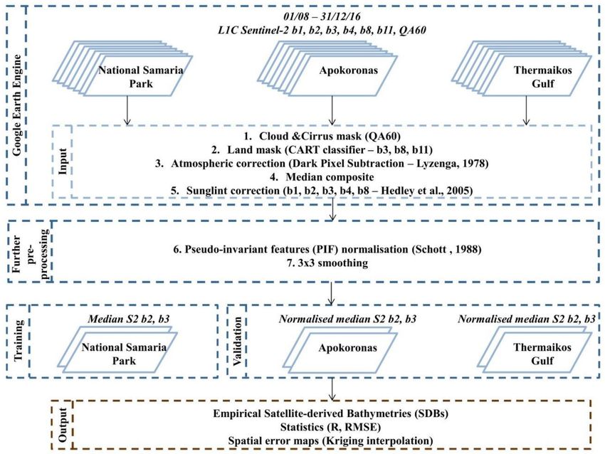
2.2. Sentinel-2 Data Preprocessing
A plethora of factors affect the state of the atmosphere (e.g., haze, aerosols, and clouds), sea surface
(e.g., sun glint, sky glint, and white caps) and water column (e.g., sedimentation, turbidity and variable
optical properties) hindering the remote sensing of the optically shallow extent (where part of the
water surface remote signal contains a bottom signal). A suitable preprocessing approach which
precedes the estimation of bathymetry from remotely sensed images should address and correct
most of these impeding factors. Google Earth Engine’s open petabyte-scale satellite image archive
allows unprecedented, on the fly, multi-image processing in the cloud. This offers the opportunity to
address the hindrances which are inherent in the nature of optically shallow water remote sensing.
As such, we implement a preprocessing workflow (Figure 2) that features a combination of metadata
information, widely used algorithms in the field of coastal aquatic remote sensing, image composition
(median composite), image normalisation, and smoothing. We applied the preprocessing workflow
on Sentinel-2 (S2) Level-1C (L1C) top of atmosphere (TOA) data which is the standard S2 archive in
GEE (ImageCollection ID: COPERNICUS/S2). Seven S2 bands (coastal aerosol: b1, blue: b2, green: b3,
red: b4, near infrared (NIR): b8, shortwave infrared (SWIR) 1: b11, quality assurance (QA) 60 band)
form this data input which spans the period between 1 August and 31 December 2016, which is close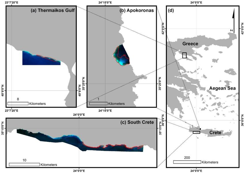
Remote Sens. 2018, 10, 859                                                                           4 of 18

chronologically to the acquisition of all in situ bathymetry data and is when the water column is better
stratified in the study areas [23]. Our preprocessing workflow consists of seven steps:

1.    We employ the QA60 bitmask band which contains cloud information to mask out opaque and
      cirrus clouds and scale S2 L1C TOA data by 10,000 (S2 quantification value).
2.    We use a classification and regression tree (CART) classifier [24] on a b3-b8-b11 composite to mask
      the terrestrial environment. It is noteworthy that although the classifier is trained with selected
      aquatic and terrestrial points (35 and 32, respectively) around Crete Island only (Figure 1d), it is
      utilised in all three sites.
3.    To atmospherically correct the masked for clouds and land images, we implement a modified
      dark pixel subtraction (DPS) method after [25] which subtracts the mean radiance of optically
      deep-water pixels (>40 m) to address path radiance and two standard deviations to address
      sensor-related noise in all bands.
4.    We employ the so-called image composition where a new pseudo-image is created using—in our
      case—the median values of the already pre-processed images [16]. This approach aims to further
      reduce image artefacts which have not been corrected by the previous preprocessing steps. In fact,
      79 tiles (34 SGE, 34 SGD, 35 SKV and 35 SKU; also called granules—100 × 100 km2 ortho images
      projected in Universal Transverse Mercator UTM/WGS84 [26]) form the Samaria National Park
      and Apokoronas pseudo-image, while 18 tiles (34 TFK) form the Thermaikos pseudo-image.
5.    We apply the sun glint correction algorithm from [27] to the median composite. Following a
      user-defined set of pixels that represents sun glint of variable intensity (two polygons in the south
      of tSamaria National Park site in South Crete), the algorithm equals the sun glint-corrected/sun
      glint-polluted median composite reduced by the product of the slope of the regression of NIR b8
      against b1–b4 and the difference between b8 and its minimum value. We should state here that
      in [28], the preprocessing step included the mean and not the minimum NIR signal over optically
      deep water. The two last steps of our preprocessing chain are performed in a GIS environment
      (ArcMap 10.5) as we export the sun glint-corrected median composites from the previous step for
      all three areas of interest.
6.    We implement the pseudo-invariant features (PIF) [21] to radiometrically normalise b2 and
      b3 bands which are used in the validation of the SDB models (Apokoronas and Thermaikos
      composites; Figure 1a,b) to the b2 and b3 of the National Samaria Park composite (Figure 1c).
      This technique was developed to quantitatively transform a subject multispectral image to the
      reference multispectral image as if they were sensed under the same atmospheric conditions,
      and in the case of a coastal study, the same water surface and column conditions. The PIF-based
      composite normalisation is employed here to decrease the spectral differences which caused high
      RMSEs in our first SDB validation experiments (results are not shown here). Figure 3 displays
      the location of the selected PIF features (44 in total for each site), with shallow sands as the
      bright features and Posidonia oceanica seagrasses (National Samaria Park and Thermaikos) and
      brown algae (Apokoronas; mainly Cystoseira sp.) as the dark features. Figure S1 shows the
      linear equations which are utilised in the radiometric normalisations. We select these specific
      features because they occupy the extremes (high, low) of the observed reflectance range in all
      three sites following the recommendations that can be found in [29]; the underlying assumption
      here is that the PIF changes little between the same tiles (=same site) and different composites
      (=different site).
7.    We apply a 3 × 3 low pass filter to the normalised S2 b2 and b3 bands to further reduce noise
      before the training and validation of the empirical SDB models.

2.3. Empirical Satellite-Derived Bathymetries (SDB)
    Generally, empirical SDB methods require certain bands in the visible wavelength, with blue
and green being the most widely used (as independent variables), and a set of known in situ depths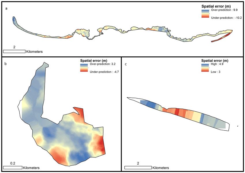
Remote Sens. 2018, 10, 859                                                                          5 of 18

(the dependent variable) as the only inputs in simple or multiple linear regressions which lead to
bathymetry estimations in a given area. Here, we implement and compare four different empirical
approaches to derive bathymetry from the pre-processed GEE Sentinel-2 composites. To be consistent
in our comparison with the other SDB models and the existing SDB literature, we exploit only the blue
and green S2 wavelengths (b2: 496.6 and b3: 560 nm for S2A) in the estimations due to their reasonable
water penetration. The training of all four models takes place in the National Samaria Park, while
the validation was performed in two different areas: the Apokoronas area and the Thermaikos Gulf
(Figure 1). Table 1 provides information on the size of the survey area, number of used in situ points,
and their depth range. Given the different depth range of the in situ points in the two validation sites
(0–25 m in Apokoronas and 0–12 m in Thermaikos), we trained two different sub-models for each one
of the four SDB methods to increase the accuracy of the estimated SDB as it is trained and validated
using the same depth range. The first and oldest approach is the one proposed by the author of [28]
(hereafter Lyzenga85) which assumes a linear relationship between the log-transformed bands and
known depth via (multiple) linear regression. The produced coefficients of the regression are then
used to train the Lyzenga85 SDB model which forms as:

                                           z = h0 + hi Xi + hj Xj                                      (1)

where z is the satellite-derived bathymetry, h0 , hi , and hj are the coefficients (intercept and slopes),
and Xi and Xj are the independent variables (the radiance in the blue and green bands, respectively).
For the 0–25-m depth range, the Lyzenga85 model features an R2 of 0.79 and RMSE of 2.46 m and takes
the form:
                                    z = −27.85 + 4.95b2 − 14.13b3                                     (2)

while for the 0–12-m depth range, the model exhibits an R2 of 0.69 and RMSE of 1.39 m:

                                      z = −7.76 + 4.76b2 − 8.71b3                                      (3)

    The second and third selected approaches follow two modifications of the proposal
by [30]—hereafter referred to as modified Stumpf03 and Traganos17 (after its first use in [31]),
respectively—concerning the empirical relationship between the ratio of the log-transformed green
band to the log-transformed blue band and water depth. The modified Stumpf03 is simply the
multiplicative inverse of the original ratio; it employs the blue to green ratio instead of the original
green to blue ratio:
                                                  ln (nb2)
                                         z = m1            − m0                                      (4)
                                                  ln (nb3)
where m1 and m0 are the slope and y-intercept, set by the linear regression between the ratio and
bathymetry, and n is a fixed constant (1000 in all experiments related to the approach in [31]) to assure
the linear response of the logarithmic ratio with depth and that it will remain positive at all points.
The m1 and m0 values are 44.39 and 33.17 for the 25-m training set (R2 = 0.59, RMSE = 3.49 m) and
20.37 and 12.16 for the 12-m training set (R2 = 0.5, RMSE = 1.78 m), respectively. The Traganos17 SDB
algorithm is essentially the ratio of log-transformed blue to log-transformed green (x) without the
n constant of Equation (4) and has shown more accurate results over low-reflectance bottoms (e.g.,
seagrasses and algae) than the original algorithm in [30], which was primarily tested in and tuned
with high-reflectance bottoms (e.g., sand, coral reefs). The exponential equation:

                                            z = 4416.3e−6.12x                                          (5)

is implemented to estimate bathymetry in the Apokoronas area (R2 = 0.67, RMSE = 3.65 m) up to a
25-m depth, while the linear equation with m1 and m0 values of 20.37 and 12.16, respectively, derives
bathymetry of up to a 12-m depth in the Thermaikos Gulf (R2 = 0.56, RMSE = 1.68 m). The fourth and
final SDB empirical approach is the one developed by the authors of [32] (hereafter Dierssen03), which
Remote Sens. 2018, 10, 859 6 of 18
takes the log-transformed ratio of the blue to green median composite (x) here (green to red band in
the original paper) to map bathymetry. The exponential equation:
z = 9.46e1.52x (6)
is used to estimate the bathymetry in Apokoronas (R2 = 0.66, RMSE = 3.59 m) in the 0–25-m depth
range and the linear equation:
b2
z = 7.05 ln ( ) + 8.31 (7)
b3
derives the bathymetry in Thermaikos in the 0–12 m depth range (R2 = 0.53, RMSE = 1.72 m).
Figure 1. Locations of selected study sites for bathymetry model analysis: (a) Thermaikos Gulf;
(b) Obros Gyalos in the Apokoronas area; (c) National Samaria Park, South Crete; and (d) the
Aegean Sea, Greece. The red polygons indicate the extent of the area that is used for the actual
analysis. All depicted images are median Sentinel-2 composites using the preprocessing workflow
from Figure 2.
2.4. Spatial Distribution of Model Residuals
As our studied seabed varies from bright shallow sand to dark seagrass meadows and
algae-covered bottoms, we expect related errors in the resulting SDB maps. To further distil the
spatial information from the SDB maps, we calculate the distribution of model residuals. We estimate
the latter as the remainder of the subtraction of the in situ bathymetry data from the most accurate
trained and validated SDB maps (Lyzenga85 in all three areas). Following the suggestions by the
authors of [33], spatial error maps are derived by Kriging interpolation (ArcMap Spatial Analyst tool)
of the remaining points to the whole extent of the training and validation sites to unveil over- and
under-prediction patterns of the SDB models. The Kriging interpolation algorithm utilises a spherical
semivariogram model and a variable search radius of 12 points to “capture both the deterministic and
autocorrelated variation in the residual surface” [33].Remote Sens. 2018, 10, 859 7 of 18
Figure 2. The methodological workflow of the present study. We employ seagrass and algae beds as
dark features and shallow sand as bright features; We perform the training of the satellite-derived
models in the National Samaria Park sites using two different depth ranges to capture the representative
depth range in the validation sites: 0–25 m in Apokoronas and 0–12 m in Thermaikos.
Figure 3. Location of used pseudo-invariant features (zoomed right panels) in the normalisation of the
Apokoronas and Thermaikos composites (b,c) to the National Samaria Park composite (a).Remote Sens. 2018, 10, 859 8 of 18
Table 1. Survey area and number of related in situ points used for training and validation of the
satellite-derived bathymetry models. The Thermaikos Gulf has a lower number of validation points as
the initially available dataset is much smaller in comparison to that of Apokoronas.
National Samaria Park Apokoronas Thermaikos Gulf
Survey Site
(Training) (Validation) (Validation)
Survey area (km2 ) 46.3 1.3 20.6
4978 (25-m models)
Number of in situ points 1557 53
3230 (12-m models)
0–25:
0–5 (675), 0–25:
5–10 (1998), 0–5 (57), 0–12
Depth range and intervals of 10–15 (1247), 5–10 (301), 0–5 (25),
in situ points (m) 15–20 (659), 10–15 (428), 5–10 (26),
20–25 (399) 15–20 (517), 10–15 (2)
0–12: 20–25 (254)
10–12 (556)
3. Results
3.1. SDB Estimations
Figure 4 shows the pre-processed median S2 composites and their respective satellite-derived
bathymetry maps of the training (Figure 4a,b) and validation sites (Figure 4b,c,e,f). Maximum SDB
depths are 27 m in National Samaria Park, 23 m in Apokoronas, and 16 m in the Thermaikos
Gulf (minimum depth of Thermaikos is 1.7 m, 0 in the two other sites). All statistical results
are collectively given in Tables S1 and S2. In terms of validation, the Lyzenga85 model achieves
the best accuracies, explaining 90% of the variation inside the validation dataset at Apokoronas
(Figure 5—1557 points; RMSE = 1.67 m) and 86% of the variation inside the validation dataset
at Thermaikos (Figure 6—53 points; RMSE = 4.1 m). More specifically, with regard to the
Apokoronas area, the Lyzenga85 approach features approximately twelve-fold higher R2 and five-fold
smaller RMSEs than the average R2 and RMSE values of 0.073 and 8.84 m, respectively, for the
modified Stumpf03, Traganos17, and Dierssen03 approaches. On the other hand, with regard to the
Thermaikos area, the Lyzenga85 model explains 2.6 times better the variation within the validation
dataset than the average 33% of the other three models, but exhibits a 1.49-m greater RMSE than their
average value of 2.6 m. The utilisation of the Traganos17 SDB model yields the lowest RMSE of 2.49 m
here (R2 = 0.52).
3.2. Methodological Gains Using a PIF Normalisation and 3 × 3 Smoothing
Figure 5 demonstrates the effectiveness of including pseudo-invariant-feature-based
normalisation and a 3 × 3 low pass filter over the remotely-sensed composite before the validation
of the SDB models. All four panels in Figure 5 are the validation plots of the model with the highest
accuracy (Lyzenga85) in the Apokoronas area which differ in terms of the incorporated preprocessing
methods. The validation on a pre-processed composite utilising only the five first steps of Figure 2
(Figure 5a) results in an R2 of 0.89 and a RMSE of 3.79 m, which is nearly halved to 1.92 m (same R2 )
by normalising the pre-processed composite prior to the validation (Figure 5b). The application of
3 × 3 smoothing without the normalisation (Figure 5c) produces the highest RMSE of 4.79 m (nearly
same R2 of 0.88), whereas with normalisation (Figure 5d), we observe that R2 rises marginally by 0.02,
and the RMSE drops to 1.67 m in comparison to step 3.Remote Sens. 2018, 10, 859 9 of 18
Figure 4. Pre-processed median Sentinel-2 composites using the workflow of Figure 2 on the left
panels (a–c) and related best empirical satellite-derived bathymetry (SDB) estimates on the right
(d–f): The National Samaria Park composite and related SDB estimates in panels (a,d); Apokoronas
composite and related SDB estimates in panels (b,e); Thermaikos composite and related SDB estimates
in panels (c,f). Red points depict the employed in situ points in the training (a) and validation (b,c)
of the SDB models here. Best algorithm (highest R2 , lowest RMSE) in all three cases is Lyzenga85
model applied on 3 × 3 smoothed and normalised median Sentinel-2 composites using the shown
pseudo-invariant (PIF) features in the zoomed maps of Figure 3b.
3.3. Spatial Distribution of Model Residuals
Figure 7 depicts the spatial variation of the model residuals of the SDB maps following training
by the Lyzenga85 model. In conjunction with the validation plots in Figures 5 and 6, the three
figures reveal potential geographical- (horizontal) and depth-related (vertical) patterns of over- or
under-prediction (always as a reference to the used in situ data) and the relation of the latter to the
presence of specific habitats. There are several distinctive over- and under-prediction SDB patterns.
First, the National Samaria Park area (training site) features an under-prediction and over-prediction
tendency in its westernmost and easternmost parts, respectively (Figure 7a). There are also model
residuals related to under-prediction over shallow sand and rocks of less than ~6 m and more than
~21 m (Figures 3a, 4d and 7a). Second, the Apokoronas area (first validation site) shows variable
prediction trends across variable depth zones—the Lyzenga85 model underpredicts bathymetry in
approximately the first 6 m over the sand-covered seabed and in the algae-covered seabed deeper than
approximately 17 m (Figures 3b, 4e and 7b). The latter is further justified by the validation plot (4)
of Figure 5 which displays an under-estimation of depth towards the deeper seabed in Apokoronas.
The remainder of the bottom of the same site—which is dominated by algae habitats—depicts an
over-prediction of SDB (Figure 7b). Third, the residuals in the Thermaikos Gulf (second validation site)
are all related to over-prediction, which ranges between 3 and 4.9 m. While the westernmost and
easternmost Thermaikos’ seabed, covered with dense P. oceanica seagrass and sparse Cymodocea nodosa
seagrass, exhibit the greatest degree of over-prediction, the central Thermaikos, covered by a smaller
P. oceanica meadow, lays out a smaller degree of over-prediction with a rising tendency from west
to east (away from the centre of the composite) (Figure 7c). Last but not least, we note mediumRemote Sens. 2018, 10, 859 10 of 18
over-prediction values (off-white colour) over the sandy bottom in the northwestern and southeastern
areas. This is greater than for the studied central Gulf.
Figure 5. Validation plots of in situ depth points (x-axis) against image-derived bathymetries (y-axis)
implementing the Lyzenga85 model which displays the best accuracy from the median Sentinel-2
composites of Apokoronas site for successive methodological steps including: (a) the initial median
Sentinel-2 composite; (b) a normalised median Sentinel-2 composite using the shown pseudo-invariant
(PIF) features in the zoomed maps of Figure 3b; (c) a 3 × 3 smoothed median Sentinel-2 composite;
(d) a 3 × 3 smoothed and normalised median Sentinel-2 composite which shows the best accuracy
among the four models of the present study in the Apokoronas site.
Figure 6. Validation plot of 53 in situ depth points (x-axis) against image-derived bathymetries (y-axis)
employing the Lyzenga85 model on the 3 × 3 smoothed and normalised median Sentinel-2 composite
of Thermaikos site.Remote Sens. 2018, 10, 859 11 of 18
Figure 7. Spatial distribution of model residuals of the SDB maps with the highest accuracy. (a) the
training site (National Samaria Park, 25-m maximum depth); (b,c) the two validation sites—Apokoronas
in panel b (25-m maximum depth) and Thermaikos in panel c (12-m maximum depth). Note that
the upper and lower left ramps indicate over- and under-prediction (as the difference between
satellite-derived and in situ bathymetry), while the lower right ramp depicts high to low spatial
error (both over-prediction).
3.4. SDB Sensitivity to Variation in Seabed Habitat and Reflectance
To further explore the performance of the SDB models with bottom habitat variability, we examine
the two most widely implemented empirical algorithms, Lyzenga85 and Stumpf03, and the blue
median reflectance composite (490 nm) along two different transects (0–20-m depth range) in the three
study areas (Figure 8). All references to panels in this paragraph are as given for those in Figure 8.
All transects run seaward and nearly perpendicularly to the coastline.
Generally, the better performance of Lyzenga85 in comparison to the modified Stumpf03 is
exemplified by the smoother variation of the former model with changes in seabed habitats and
thus more blue reflectance than in the latter model. Stumpf03 and blue reflectance appear to be
more dependent across the majority of transects; at the same time, the Lyzenga85 model exhibits
a smaller habitat interdependence (as manifested by variations of blue reflectance), especially over
dark-reflectance bottom areas (seagrass and algae) as seen in the upper left (240–500 m), middle right,
and lower left panels. Additionally, in comparison to Stumpf03, Lyzenga85 seems to underpredict
bathymetry over sandy and rocky habitats, except for the deeper sand (b2 < ~0.015) (upper left and
right, middle left, and lower left panels).Remote Sens. 2018, 10, 859 12 of 18
Figure 8. Satellite-derived bathymetry profiles using most accurate Lyzenga85 and modified Stumpf03
models, and a 3 × 3 smoothed and normalised median blue Sentinel-2 reflectance composite (490 nm).
(A) Samaria National Park: profile over seabed with rocks, sand, and Posidonia oceanica seagrass,
successively; (B) Samaria National Park: profile over sand; (C,D) the Apokoronas site: profiles over
sand and algae-covered beds, respectively; (E,F) Thermaikos site: profiles over sand and P. oceanica
seagrass, respectively.
4. Discussion
4.1. Cloud-Based SDB and Model Performance
Cloud-based geospatial analysis platforms, such as the herein utilised Google Earth Engine,
provide an unprecedented opportunity for large-scale, on the fly preprocessing, processing,
and analysis of vital to the coastal marine environment open data. Here, we developed a preprocessing
workflow within GEE and a GIS environment which implements a plethora of widely used and well
established algorithms in the remote sensing of optically shallow habitats (seagrasses, corals, algae etc.)Remote Sens. 2018, 10, 859 13 of 18
prior to the calculation of four empirical satellite-derived bathymetries [28,30–32] with Sentinel-2 along
with their statistics and model residuals.
During the last three decades, a series of empirical, semi-analytical, and analytical methods have
been developed for the estimation of optically shallow bathymetry from remote sensing images [34].
Here, we focus on the empirical methodologies which employ linear- or ratio-based statistical
relationships between the log-transformed, water-penetrating bands (most frequently at blue and green
wavelengths) and acoustic-derived in situ depth data to calculate SDB. Empirical algorithms assume
a priori homogeneous water column and bottom composition; this is rarely the case, however, in a
typical coastal Aegean benthic site with several seagrasses neighbouring sands and rocks with algal
communities within the optical depth limit of the herein used Sentinel-2. Therefore, the non-unique
nature of our selected study sites somehow breaches the assumptions of the empirical approaches.
Nevertheless, we examine them here due to their historical significance, simple and widespread
utilisation, and good accuracy. Among the investigated models in both training and validation in the
two depth ranges (0–12 and 0–25 m), the Lyzenga85 model [28] exhibits the highest R2 and smaller
RMSE values on average (0.81 and 2.4 m respectively) followed by the Traganos17 model [31] with
an R2 of 0.45 and RMSE of 4.03 m. The empirical model of Stumpf03 features the poorest overall
performance with an R2 of 0.3 and RMSE of 4.41 m (Table S1 and S2). All models are tuned in the
National Samaria Park over primarily sand- and rocky-covered seabed with sparse seagrass patches
and validated over the mainly sandy bottom with a few algae in Apokoronas and the dense seagrass
beds with few sands and algae in the Thermaikos Gulf (Figure 4). In comparison to unpublished
SDB results in the South Cretan training site using the Dierssen03 [33] empirical band ratio of a
super-resolved (60 to 10 m) Sentinel-2 coastal aerosol band 1 to green band 3 tuned with the same in
situ depth data with the present study (depth range of 0–30 m), the herein Dierssen03 model produces
a lower lower R2 (reduced by 0.19), but also 0.72-m smaller RMSE.
On the other hand, previously published SDB results using Sentinel-2 in the validation site of the
Thermaikos [31] with the original Traganos17 algorithm tuned in the same waters at depths between
0 and 20 m explained 1.76 times better the variation, with a 1.19-m smaller RMSE in comparison to
the present Traganos17 results. In yet another SDB application in the Thermaikos site [34] with 5-m
RapidEye imagery, the use of Dierssen03 empirical ratio exhibited a 0.49 lower R2 with a decreased
RMSE of 0.09 m in comparison to the herein validated Dierrsen03 model. In the previous approaches,
training and validation data points originated from the same site and thus were characterised by
high autocorrelation according to the first law of geography by Tobler which could have caused
statistical bias; here, we attempt to lower this bias by employing two independent in situ data sets in
two different sites to validate the calibrated empirical models.
4.2. On the Importance of Image Composition, PIF and the Spatial Distribution of Errors
The ability to create remotely sensed image composites by calculating the median of every pixel
in the image across a given time range mitigates in an inter-image fashion intra-image issues related
to water surface and water quality conditions, and optical properties; issues like waves, sun glint
and sky glint, temporal sedimentation due to land-based rainfall runoffs, or resuspension of seabed
sediments due to intensive wave activity for long periods tend to degrade the quality of single images
and impede SDB applications. The selected time range affects the composite quality—a short time
range could possibly cause data gaps while a long one could amplify the artificiality of the resulting
pseudo-image. Here, we selected the time period between 1 August and 31 December 2016, which is
chronologically closer to the acquisition of field bathymetry data within the Sentinel-2 lifespan and
satisfies the criterion of a better-stratified water column for our study region (Aegean Sea) [23]. Future
users of the herein proposed workflow are naturally expected to choose the time range based on the
acquisition dates of their in situ data, and the optimum surface and water column conditions of their
study area. It is worth mentioning that the temporal difference between data acquisition (2012–2015)
and image composition (2016) in our study is not expected to obstruct the SDB estimations becauseRemote Sens. 2018, 10, 859 14 of 18
all three sites are relatively protected from both weather phenomena and coastal processes, hence
featuring a stable seabed. While the present work is within a coastal marine environment with almost
no influence from tides, when the used methods and the proposed approaches are adopted at areas
with tides that affect the results, a correction of the tide using measurements from tide gauges at fixed
stations is a mandatory step in the satellite derived bathymetry process.
The radiometric normalization of the median image composites using the pseudo-invariant-feature
approach [21] allows the successful development of our approach. The implemented image composites
for validation here originate in sites which are approximately 26 (Apokoronas) and 562 km (Thermaikos)
(Figure 1) away from the training site (National Samaria Park). This necessitates the utilisation of the PIF
normalisation method to correct the two former composites to the reflectance range of the latter composite.
The yielded better statistics following utilisation of PIF and 3 × 3 low pass in combination with the smaller
spread of regressed values (Figure 5d) manifest the importance of these two preprocessing steps. The
image composition using median values prior to the application of PIF increases the reliability of the
subsequent SDB estimations due to the decrease of cross-image composite comparison issues [35]. To the
best of our knowledge, this study is the first to employ PIF as a preprocessing step for SDB calculations.
Previous uses of PIF normalisation within an optically coastal shallow setting have been confided to its
preprocessing implementation for coral bleaching detection [29,36].
The depiction of the spatial distribution of model residuals (Figure 7) is integral here. There
are two inherent assumptions in the empirical nature of SDB estimations; first, in situ observations
employed in the training and validation of a given SDB model are independent in between them,
and second, model residuals feature a normal distribution and random location. The presence of spatial
dependence shown by the selection of observations from the same image (and thus in close proximity)
adheres to the first law of geography by Tobler but violates the assumed freedom and location of in
situ measurements, heightening the standard error and broadly lowering the statistical confidence of
the SDB models. On one hand, the origination of both training and validations datasets from the same
site is common practice in optically shallow bathymetry derivation studies due to practical reasons
(usually the high cost of acquiring such data in the field). On the other hand, the existence of three
in situ single beam-derived bathymetry datasets allows us to confront the aforementioned violation,
subsequently restricting statistical bias in the results.
The spatial error maps unveil specific over- and under-prediction patterns. Demonstrated more
pronouncedly in the National Samaria Park and Apokoronas sites (upper and lower left panel in
Figure 7), we identify that mainly algae-covered beds relate to an over-prediction tendency because
they comprise a low-reflectance habitat. In the very shallow pixels of Apokoronas, there might be an
over-correction by the sun glint algorithm found in [26] due to the interaction of light photons with
the seabed in the NIR wavelength which may have decreased reflectance composite values and added
to the over-prediction trends. On the contrary, sandy and rocky bottoms reflect more photons, hence
producing under-prediction patterns. Generally, the number of photons which reflect on the seabed
decreases, and reaches zero past a certain depth limit as averaged by the herein image composition.
At this point, the remote sensing signal would contain information arising only from the water column
and not the water bottom, therefore being unable to estimate bathymetry. This could have caused
the visible under-prediction patterns towards deeper areas independent of the underlying habitat as
manifested by the fourth panel in Figure 5 (beyond ~22 m), and the upper and lower left panel in
Figure 7 (red colours).
We also show the importance of using the same depth ranges of in situ data for both training
and validation of our SDB models, which increase R2 and decrease RMSE. Implementation of the
0–25 m training in National Samaria Park, validated in the Apokoronas site model in the Thermaikos
site and spanning depths of up to 12 m, produces a 0.06 smaller R2 value and a nearly two-fold
smaller RMSE than the final trained Lyzenga85 model within 0–12 m (Figure 6). This has been also
mentioned in [34]: “The optimal performance of bathymetric estimates is like to be achieved when points
covering a fully-representative range of depths are present in both datasets”.Remote Sens. 2018, 10, 859 15 of 18
4.3. In Situ Data Collection, Crowdsourced Information and an Outlook for SDB
A vital feature of the present study is the use of low-cost tools for the collection of in situ
bathymetric data. Usually, such data are collected by expensive state-of-the-art equipment such
as airborne lidar data [37] or multibeam echosounder systems [38]. While these tools derive very
high-resolution bathymetries, both their spatial coverage and updating of the derived bathymetry
are limited and particularly costly at the shallow coastal zone which is practically inaccessible for
large boats carrying the acoustic equipment and where the multibeam swath is narrow. Additionally,
airborne campaigns require special licenses that are difficult to obtain. Here, we employ commercial
off-the-shelf (COTS) solutions with a total cost of less than 1500 euros, which can be utilised at any
region of interest.
Another method of in situ data collection is the involvement of crowdsourcing/citizen science data
collection methodology [39]. Since 1963, the Cooperative Charting Program between NOAA’s Office of
Coast Survey and the United States Power Squadron (USPS) has triggered the submission of bathymetric
point data to cartographers via the postal service for chart application. Up to today, several initiatives
based on the voluntary participation of boat owners with installed hydrographic equipment have been
released [35,40], resulting in the provision of bathymetric maps and information on bottom type and
vegetation cover in some cases. Most recently, the Nippon Foundation General Bathymetric Chart of the
Oceans (GEBCO) Seabed 2030 project was launched at the United Nations Oceans Conference in 2017
with the goal to map the entirety of the world’s ocean seabed by 2030. To achieve this unquestionably
ambitious goal, the project aims to create a new fleet of research vessels by employing millions of fishing
boats, thousands of cargo, cruise, and passenger ships, and private yachts to acquire crowdsourcing
multibeam echosounder data [41]. Nonetheless, the extraction of raw data (XYZ) from the existing
databases is not yet permitted for the public, but companies and research projects—such as the H2020
BASE-platform (https://base-platform.com/)—have reached an agreement and the first SDB results
utilising crowdsourcing data are now available. The accessibility of such raw data is crucial towards a new
era for global coastal bathymetry applications using the present proposed methodology. The empirical
nature of our methodology, however, raises the computational demands within the GEE due to the
estimation of the regressions between the image composition values and water depth—large scales in
both space and time could cause the GEE to create a time-out (GEE error message).
In addition to the envisioned new era for large-scale bathymetry, we discuss five near-future endeavours
which could directly or indirectly succeed and/or improve the present methodology and study:
1. The implementation of the estimated spatial error parameter as a postprocessing step to increase
the statistical accuracy of the empirically derived SDB models following the work in [34].
2. The utilisation of best-available-pixel (BAP) composition, which employs a series of pixel-based
scores related to distance to clouds and shadow masks, atmospheric opacity, day of the year etc.,
instead of image composition across a relevant time series to the user’s study region [42].
3. The use of the proposed preprocessing workflow to conduct sea- to basin-wide habitat mapping
and monitoring.
4. The incorporation of radiative transfer-based optimisations following the semi-analytical
inversion method of [43] or machine learning methods [10,44] for the derivation of bathymetry.
5. The fusion of the Copernicus Sentinel-1 (also available in GEE) and the Sentinel-2 open and
free image archive for the development of 10-m topobathymetric digital elevation models
(DEMs)—seamless merged elevation products of terrestrial and underwater topography [45]
useful for numerous Earth science applications including mapping and modelling of inundation,
sediment transport, sea-level rise, and storm surge [46].
5. Conclusions
The present study proposes a complete preprocessing chain in Google Earth Engine—including
simple and well-established algorithms in the remote sensing of optically shallow habitats—whichRemote Sens. 2018, 10, 859 16 of 18
could be easily implemented through the online provided code to estimate satellite-derived bathymetry
using Sentinel-2 data and low-cost field data. The user can select a suitable time range of available
Sentinel-2 images according to the available in situ depth data and optimum surface and water column
conditions of the area of interest. Here, we train four SDB models utilising a pre-processed median
composite of 79 S2 tiles in SW Crete (Eastern Mediterranean) and validate them employing 79- and
18-tile composites in NW Crete and the NW Aegean Sea, 26 and 562 km away, respectively. Given
the good accuracies of the calibrated model in the two validation sites (R2 up to 0.9 and RMSE as
low as 1.67 m) despite the large horizontal distance, there is emerging potential for upscaling the
herein developed SDB model to the whole optically shallow extent of the Aegean and Ionian Seas,
hence further exploiting the capability of GEE for big data analysis. To this end, one particular
challenge would surely be the existence of relevant field bathymetric data to validate the accuracy
of the upscaling effort. The innovation of this work lies mainly in the fact that it is the first that
implements the inter-image approach of image composition within GEE to address single-image issues
like atmospheric, surface, and water column interferences which obstruct space-borne approaches
in the field of aquatic remote sensing. Moreover, in comparison to their exclusion, the inclusion of
PIF-based normalisation to match the reflectance range of the training composite to the validation
composites along with a 3 × 3 smoothing to filter remaining noise prior to the SDB calculation
notably improve the methodology as manifested by the increased SDB accuracies. On the other hand,
regressions which lie in the heart of the empirical models (e.g., sun glint correction, PIF normalisation,
SDB estimations) decrease processing time in GEE and could possibly create related time-out errors.
This led us to conduct the radiometric normalisation and the SDB calculations outside GEE in this
study for the sake of efficiency. In the near future, we aim to integrate these two preprocessing and
analysis steps within the GEE platform in addition to adapting the code to also use Landsat 8 images
as input. All in all, due to intense anthropogenic activities, coastal ecosystems are on the verge of
significant degradation of their ecosystem services; however, Google Earth Engine and Sentinel-2 have
created the perfect storm in the last three years for an unprecedented, global-scale, high spatiotemporal
mapping of bathymetry and, more broadly, of the immensely vital optically shallow benthos which
can in turn empower physical understanding, management and conservation practices.
Supplementary Materials: The following are available online at http://www.mdpi.com/2072-4292/10/6/859/
s1.
Author Contributions: D.T. and D.P. conceived the idea, collected the in-situ data, processed the satellite-derived
bathymetries, and wrote the paper; B.A. developed the preprocessing code in Google Earth Engine; P.R. and N.C.
supervised the development of the present project, from start to finish.
Acknowledgments: D.P. and N.C. are supported by the European H2020 Project 641762 ECOPOTENTIAL:
Improving future ecosystem benefits through Earth Observations. D.T. is supported by a DLR-DAAD Research
Fellowship (No. 57186656).
Conflicts of Interest: The authors declare no conflict of interest.
References
1. Paterson, D.M.; Hanley, N.D.; Black, K.; Defew, E.C.; Solan, M. (Eds.) Biodiversity, ecosystems and coastal zone
management: Linking science and policy. Theme Section. Mar. Ecol. Prog. Ser. 2011, 434, 201–301. [CrossRef]
2. Robertson, E. Crowd-Sourced Bathymetry Data via Electronic Charting Systems. ESRI Ocean GIS Forum,
2016. Available online: http://proceedings.esri.com/library/userconf/oceans16/papers/oceans_12.pdf
(accessed on 20 April 2018).
3. Li, R.; Liu, J.-K.; Felus, Y. Spatial Modeling and Analysis for Shoreline Change Detection and Coastal Erosion
Monitoring. Mar. Geod. 2010, 24, 1–12. [CrossRef]
4. Omira, R.; Baptista, M.A.; Leone, F.; Matias, L.; Mellas, S.; Zourarah, B.; Miranda, J.M.; Carrilho, F.; Cherel, J.P.
Performance of coastal sea-defense infrastructure at El Jadida (Morocco) against tsunami threat: Lessons
learned from the Japanese 11 March 2011 tsunami. Nat. Hazards Earth Syst. Sci. 2013, 13, 1779–1794.
[CrossRef]Remote Sens. 2018, 10, 859 17 of 18
5. Roelfsema, C.; Kovacs, E.; Ortiz, J.C.; Wolff, N.H.; Callaghan, D.; Wettle, M.; Ronan, M.; Hamylton, S.M.;
Mumby, P.J.; Phinn, S. Coral reef habitat mapping: A combination of object-based image analysis and
ecological modelling. Remote Sens. Environ. 2018, 208, 27–41. [CrossRef]
6. Wang, J.; Yi, S.; Li, M.; Wang, L.; Song, C. Effects of sea level rise, land subsidence, bathymetric change and
typhoon tracks on storm flooding in the coastal areas of Shanghai. Sci. Total Environ. 2018, 621, 228–234.
[CrossRef] [PubMed]
7. Sandwell, D.T.; Smith, W.H. Marine gravity anomaly from Geosat and ERS 1 satellite altimetry. J. Geophys.
Res. Solid Earth 1997, 102, 10039–10054. [CrossRef]
8. Olson, C.J.; Becker, J.J.; Sandwell, D.T. A new global bathymetry map at 15 arcsecond resolution for resolving
seafloor fabric: SRTM15_PLUS. In Proceedings of the AGU Fall Meeting Abstracts, San Francisco, CA, USA,
15–19 December 2014.
9. Pe’eri, S.; Madore, B.; Nyberg, J.; Snyder, L.; Parrish, C.; Smith, S. Identifying bathymetric differences over
Alaska’s North Slope using a satellite-derived bathymetry multi-temporal approach. J. Coast. Res. 2016, 76,
56–63. [CrossRef]
10. Misra, A.; Vojinovic, Z.; Ramakrishnan, B.; Luijendijk, A.; Ranasinghe, R. Shallow water bathymetry
mapping using Support Vector Machine (SVM) technique and multispectral imagery. Int. J. Remote Sens. 2018.
[CrossRef]
11. Pacheco, A.; Horta, J.; Loureiro, C.; Ferreira, Ó. Retrieval of nearshore bathymetry from Landsat 8 images:
A tool for coastal monitoring in shallow waters. Remote Sens. Environ. 2015, 159, 102–116. [CrossRef]
12. Dörnhöfer, K.; Göritz, A.; Gege, P.; Pflug, B.; Oppelt, N. Water Constituents and Water Depth Retrieval from
Sentinel-2A—A First Evaluation in an Oligotrophic Lake. Remote Sens. 2016, 8, 941. [CrossRef]
13. Chybicki, A. Mapping South Baltic Near-Shore Bathymetry Using Sentinel-2 Observations. Pol. Mar. Res.
2017, 24, 15–25. [CrossRef]
14. Chybicki, A. Three-Dimensional Geographically Weighted Inverse Regression (3GWR) Model for Satellite
Derived Bathymetry Using Sentinel-2 Observations. Mar. Geod. 2017, 41, 1–23. [CrossRef]
15. Gorelick, N.; Hancher, M.; Dixon, M.; Ilyushchenko, S.; Thau, D.; Moore, R. Google Earth Engine:
Planetary-scale geospatial analysis for everyone. Remote Sens. Environ. 2017, 202, 18–27. [CrossRef]
16. Robinson, N.P.; Allred, B.W.; Jones, M.O.; Moreno, A.; Kimball, J.S.; Naugle, D.E.; Erickson, T.A.;
Richardson, A.D. A Dynamic Landsat Derived Normalized Difference Vegetation Index (NDVI) Product for
the Conterminous United States. Remote Sens. 2017, 9, 863. [CrossRef]
17. Xiong, J.; Thenkabail, P.S.; Tilton, J.C.; Gumma, M.K.; Teluguntla, P.; Oliphant, A.; Congalton, R.G.; Yadav, K.;
Gorelick, N. Nominal 30-m Cropland Extent Map of Continental Africa by Integrating Pixel-Based and
Object-Based Algorithms Using Sentinel-2 and Landsat-8 Data on Google Earth Engine. Remote Sens. 2017,
9, 1065. [CrossRef]
18. Parastatidis, D.; Mitraka, Z.; Chrysoulakis, N.; Abrams, M. Online Global Land Surface Temperature
Estimation from Landsat. Remote Sens. 2017, 9, 1208. [CrossRef]
19. Chrysoulakis, N.; Mitraka, Z.; Gorelick, N. Exploiting satellite observations for global surface albedo trends
monitoring. Theor. Appl. Climatol. 2018. accepted.
20. Tobler, W.R. A computer movie simulating urban growth in the detroit region. Econ. Geogr. 1970, 46, 234–240.
[CrossRef]
21. Schott, J.R.; Salvaggio, C.; Vochok, W.J. Radiometric scene normalization using pseudo-invariant features.
Remote Sens. Environ. 1988, 26, 1–16. [CrossRef]
22. Poursanidis, D.; Topouzelis, K.; Chrysoulakis, N. Mapping coastal marine habitats and delineating the
deep limits of the Neptune’s seagrass meadows using Very High Resolution Earth Observation data. Int. J.
Remote Sens. 2018. accepted.
23. Tanhua, T.; Hainbucher, D.; Schroeder, K.; Cardin, V.; Álvarez, M.; Civitarese, G. The Mediterranean Sea
system: A review and an introduction to the special issue. Ocean Sci. 2013, 9, 789–803. [CrossRef]
24. Breiman, L.; Friedman, J.H.; Olshen, R.A.; Stone, C.J. Classification and Regression Trees; Chapman & Hall/CRC:
Boca Raton, FL, USA, 1984.
25. Armstrong, R.A. Remote sensing of submerged vegetation canopies for biomass estimation. Int. J.
Remote Sens. 1993, 14, 621–627. [CrossRef]
26. European Space Agency (ESA). SENTINEL-2 User Handbook; ESA: Paris, France, 2015; p. 64.Remote Sens. 2018, 10, 859 18 of 18
27. Hedley, J.D.; Harborne, A.R.; Mumby, P.J. Technical note: Simple and robust removal of sun glint for mapping
shallow-water benthos. Int. J. Remote Sens. 2005, 26, 2107–2112. [CrossRef]
28. Lyzenga, D.R. Shallow-water bathymetry using combined lidar and passive multispectral scanner data.
Int. J. Remote Sens. 1985, 6, 115–125. [CrossRef]
29. Elvidge, C.D.; Dietz, J.B.; Berkelmans, R.; Andréfouët, S.; Skirving, W.; Strong, A.E.; Tuttle, B.T. Satellite
observation of Keppel Islands (Great Barrier Reef) 2002 coral bleaching using IKONOS data. Coral Reefs 2004,
23, 461–462. [CrossRef]
30. Stumpf, R.P.; Holderied, K.; Sinclair, M. Determination of water depth with high-resolution satellite imagery
over variable bottom types. Limnol. Oceanogr. 2003, 48, 547–556. [CrossRef]
31. Traganos, D.; Reinartz, P. Mapping Mediterranean seagrasses with Sentinel-2. Mar. Pollut. Bull. 2017.
[CrossRef] [PubMed]
32. Dierssen, H.M.; Zimmerman, R.C.; Leathers, R.A.; Downes, T.V.; Davis, C.O. Ocean color remote sensing
of seagrass and bathymetry in the Bahamas Banks by high- resolution airborne imagery. Limnol. Oceanogr.
2003, 48, 444–455. [CrossRef]
33. Hamylton, S.M.; Hedley, J.D.; Beaman, R.J. Derivation of High-Resolution Bathymetry from Multispectral
Satellite Imagery: A Comparison of Empirical and Optimisation Methods through Geographical Error
Analysis. Remote Sens. 2015, 7, 16257–16273. [CrossRef]
34. Traganos, D.; Reinartz, P. Interannual Change Detection of Mediterranean Seagrasses Using RapidEye Image
Time Series. Front. Plant Sci. 2018, 9. [CrossRef] [PubMed]
35. TeamSurv, 2018. Available online: https://www.teamsurv.com/ (accessed on 28 Match 2018).
36. Hedley, J.D.; Roelfsema, C.M.; Chollett, I.; Harborne, A.R.; Heron, S.F.; Weeks, S.; Skirving, W.J.; Strong, A.E.;
Eakin, C.M.; Christensen, T.R.L.; et al. Remote Sensing of Coral Reefs for Monitoring and Management:
A Review. Remote Sens. 2016, 8, 118. [CrossRef]
37. Saylam, K.; Hupp, J.R.; Averett, A.R.; Gutelius, W.F.; Gelhar, B.W. Airborne lidar bathymetry: Assessing
quality assurance and quality control methods with Leica Chiroptera examples. Int. J. Remote Sens. 2018, 39,
2518–2542. [CrossRef]
38. Ierodiaconou, D.; Schimel, A.C.G.; Kennedy, D.; Rattray, A. Combining pixel and object based image analysis
of ultra-high resolution multibeam bathymetry and backscatter for habitat mapping in shallow marine
waters. Mar. Geophys. Res. 2018, 39, 271. [CrossRef]
39. International Hydrographic Organization. Guidance on Crowdsourced Bathymetry; IHO, Monaco Cedex, 2018;
p. 55. Available online: https://www.iho.int/iho_pubs/draft_pubs/CSB-Guidance_Document-Ed1.0.0.pdf
(accessed on 20 April 2018).
40. BioBase, 2018. Available online: https://www.cibiobase.com/ (accessed on 28 Match 2018).
41. Nippon Foundation-GEBCO, 2018. Available online: https://seabed2030.gebco.net/ (accessed on 2 May 2018).
42. White, J.C.; Wulder, M.A.; Hobart, G.W.; Luther, J.E.; Hermosilla, T.; Griffiths, P.; Coops, N.C.; Hall, R.J.;
Hostert, P.; Dyk, A.; et al. Pixel-based image compositing for large-area dense time series applications and
science. Can. J. Remote Sens. 2014, 40, 192–212. [CrossRef]
43. Lee, Z.P.; Carder, K.L.; Mobley, C.D.; Steward, R.G.; Patch, J.S. Hyperspectral remote sensing for shallow
waters: 2. Deriving bottom depths and water properties by optimization. Appl. Opt. 1999, 38, 3831–3843.
[CrossRef] [PubMed]
44. Danilo, C.; Melgani, F. Wave period and coastal bathymetry using wave propagation on optical images.
IEEE Trans. Geosci. Remote Sens. 2016, 54. [CrossRef]
45. Collin, A.; Hench, J.L.; Pastol, Y.; Planes, S.; Thiault, L.; Schmitt, R.J.; Holbrook, S.J.; Davies, N.; Troyer, M.
High resolution topobathymetry using a Pleiades-1 triplet: Moorea Island in 3D. Remote Sens. Environ. 2018,
208, 109–119. [CrossRef]
46. Poursanidis, D.; Chrysoulakis, N. Remote Sensing, natural hazards and the contribution of ESA Sentinels
missions. Remote Sens. Appl. Soc. Environ. 2017, 6, 25–38. [CrossRef]
© 2018 by the authors. Licensee MDPI, Basel, Switzerland. This article is an open access
article distributed under the terms and conditions of the Creative Commons Attribution
(CC BY) license (http://creativecommons.org/licenses/by/4.0/).You can also read