Evaluating Collaborative Filtering Algorithms for Music Recommendations on Chinese Music Data

Evaluating Collaborative Filtering Algorithms for Music
 Recommendations on Chinese Music Data

 By
 Yifan He

 An Undergraduate Senior Honors Thesis
 Presented to the faculty
 Of the University of North Carolina at Chapel Hill
 In Partial fulfillment of the requirements
For the Honors Carolina Senior Thesis in the School of Information and Library Science

 Chapel Hill
 2021

 Approved by:
 Dr. Jaime Arguello, Thesis Advisor
 Dr. Stephanie W. Haas, Reader
 Dr. Ryan Shaw, Reader

2

© Copyright by Yifan He, 2021.

 All Rights Reserved

3

Contents

CONTENTS ............................................................................................................................. 3
LIST OF FIGURES ................................................................................................................. 5
LIST OF TABLES ................................................................................................................... 6
1. INTRODUCTION ........................................................................................................... 7
2. RELATED WORKS ...................................................................................................... 12
 2.1 INTRODUCTION ......................................................................................................... 12
 2.2 THREE TYPES OF MUSICAL METADATA .................................................................... 12
 2.3 MUSIC CONTENT-BASED METHODS .......................................................................... 13
 2.4 MUSIC CONTEXT-BASED METHODS .......................................................................... 14
 2.5 USER CONTEXT-BASED METHODS ............................................................................ 16
 2.5.1 Collaborative Filtering ........................................................................................ 16
 2.5.2 Explicit and Implicit User Feedback ................................................................... 16
 2.5.3 Memory-based Collaborative Filtering ............................................................... 17
 2.5.3.1 User-based Collaborative Filtering .............................................................. 18
 2.5.3.2 Item-based Collaborative Filtering .............................................................. 19
 2.5.4 Model-based Collaborative Filtering .................................................................. 21
 2.5.4.1 Matrix Factorization-based Collaborative Filtering..................................... 21
 2.5.5 Users’ Interactions with Recommender Systems ................................................. 22
 2.6 CONCLUSION............................................................................................................. 23
3. METHODOLOGY ........................................................................................................ 24
 3.1 DATASET .................................................................................................................. 24
 3.1.1 Parse Dataset ....................................................................................................... 26
 3.1.2 Format Dataset for Recommender System .......................................................... 27
 3.2 MODELS .................................................................................................................... 29
 3.2.1 Notation Schema .................................................................................................. 31
 3.2.2 Baselines .............................................................................................................. 32
 3.2.2.1 Min Predictor ............................................................................................... 32
 3.2.2.2 Max Predictor............................................................................................... 32
 3.2.2.3 Normal Predictor.......................................................................................... 32
 3.2.3 kNN-based Models ............................................................................................... 33
 3.2.3.1 kNN Basic..................................................................................................... 34
 3.2.3.2 kNN With Normalization ............................................................................. 34
 3.2.3.2.1 kNN with Means........................................................................................... 34
 3.2.3.2.2 kNN with Z-Score......................................................................................... 35
 3.2.3.3 Similarity Metrics for kNN Models.............................................................. 36
 3.2.3.3.1 Cosine Similarity ......................................................................................... 37
 3.2.3.3.2 Mean Squared Difference ............................................................................ 38
 3.2.3.3.3 Pearson Correlation Coefficient ................................................................... 39
 3.2.4 Slope One ............................................................................................................. 40
 3.2.5 Matrix Factorization Models ............................................................................... 42

4

 3.2.5.1 SVD .............................................................................................................. 42
 3.2.5.2 SVD++ ......................................................................................................... 44
 3.3 EVALUATIONS ........................................................................................................... 46
 3.3.1 Mean Squared Error (MSE)................................................................................. 46
 3.3.2 Root Mean Squared Error (RMSE)...................................................................... 46
 3.3.3 Mean Absolute Error (MAE) ............................................................................... 47
 3.3.4 Fraction of Concordant Pairs (FCP) .................................................................. 47
4. RESULTS AND DISCUSSION .................................................................................... 49
 4.1 BASELINES ................................................................................................................ 52
 4.2 KNN-BASED ALGORITHMS ........................................................................................ 55
 4.3 SLOPE ONE ALGORITHM ........................................................................................... 57
 4.4 MATRIX FACTORIZATION-BASED ALGORITHMS ........................................................ 58
 4.5 LIMITATIONS............................................................................................................. 59
5. CONCLUSION AND FUTURE WORKS ................................................................... 61
BIBLIOGRAPHY .................................................................................................................. 64
APPENDIX ............................................................................................................................. 69

5

List of Figures

Figure 1.1 Features of music content-based, music context-based and user context-based
approaches.................................................................................................................................. 8
Figure 2.1 User-based Collaborative Filtering Logic Flow .................................................... 19
Figure 2.2 Item-based Collaborative Filtering Logic Flow .................................................... 20
Figure 3.1 Interface of NetEase Cloud Music’s Homepage ................................................... 25
Figure 3.2 Interface of a single playlist................................................................................... 25
Figure 3.3 Sample MovieLens dataset format ........................................................................ 28
Figure 3.4 Logic flow for Slone One method ......................................................................... 41
Figure 3.5 Logic flow for SVD method .................................................................................. 43
Figure 4.1 Comparing all models on RMSE ........................................................................... 50
Figure 4.2 Comparing all models on MSE ............................................................................. 51
Figure 4.3 Comparing all models on MAE ............................................................................. 51
Figure 4.4 Comparing all models on FCP............................................................................... 52
Figure 4.5 Comparing user-based kNN models on Cosine ..................................................... 53
Figure 4.6 Comparing item-based kNN models on Cosine .................................................... 54
Figure 4.7 Comparing user-based kNN models on MSD ....................................................... 54
Figure 4.8 Comparing item-based kNN models on MSD ....................................................... 54
Figure 4.9 Comparing user-based kNN models on Pearson ................................................... 55
Figure 4.10 Comparing item-based kNN models on Pearson ................................................. 55

6

List of Tables

Table 3.1 Sample format of a Playlist ..................................................................................... 27
Table 3.2 Sample format of our dataset following MovieLens............................................... 29
Table 3.3 Models used in our experiment ............................................................................... 30
Table 3.4 Notation Schema ..................................................................................................... 31
Table 3.5 Similarity Metrics for kNN Models ........................................................................ 36
Table 4.1 Experiment results for all models ........................................................................... 49

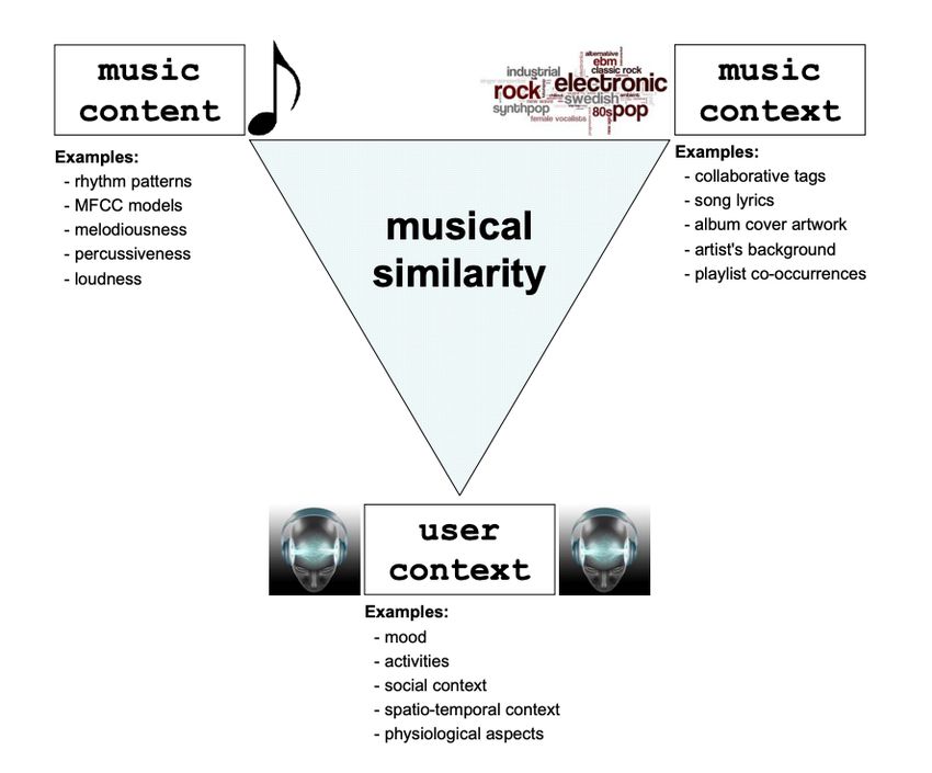
7

1. Introduction

The amount of digital music available has overwhelmingly increased during the last few

decades with the development of Internet and music technology. The use of digital music

platforms has gradually replaced many traditional music consumption methods, such as tapes,

CDs, and vinyl records. The explosive growth of digital music requires powerful knowledge

management techniques and tools. Without these tools, users will face a vast music catalog that

cannot be fully utilized. The research on Music Information Retrieval (MIR) is dedicated to

solving these problems.

 As a subfield of multimedia Information Retrieval, MIR is a highly dynamic and

multidisciplinary field of research relates to various other research disciplines, involving

researchers from the disciplines of musicology, library and information science, cognitive

science, computer science, electrical engineering, and so on. Narrowing the focus on

information retrieval (IR) and information representation related to music, we can distinguish

three broad categories of strategies in terms of their data source: music content-based, music

context-based and user context-based approaches. The music content-based approach extract

music features from the audio signal itself, such as rhythm patterns, melodies, chords

progressions, loudness, and so on. The music context-based approaches make use of text-based

data related to music, such as the performer’s background, the song’s lyrics, images of album

cover, or co-occurrence information derived from playlists. The user context-based approaches

put focuses on users’ personal data, such as their mood, physiological and spatial-temporal

context, listening pattern and history, and so on. The following Figure 1.1 show their difference.

8

 Figure 1.1 Features of music content-based, music context-based and user context-based
 approaches

In the user scenarios of digital music, many user requirements are proposed, including music

identification, query by humming, auto music transcription and alignment, and so on. Among

all these tasks, music recommendation is one of the most important and challenging tasks:

recommending music for each user in a personalized way. MIR researchers use various music-

related metadata to process and build algorithms to address this task. The state-of-the-art

approaches to music recommendation are based on measuring music similarity between raw

audio tracks, music-related metadata on the Web, and users’ profiles, eliciting similar music.

In these ways, all content-based audio features, text-based music-related metadata, and user-

based community metadata can be used. By using different types of data, several approaches

were developed respectively. Using user-based community metadata, the most used one is

9

Collaborative Filtering (CF), which analyzes one single user's behavior and compares it to other

similar users’ behaviors. The trick here is that it recommends new things based on the similarity

between users’ behaviors, not between items’ intrinsic properties. The second method, using

music content-based audio features, is the music content-based model. It analyzes to determine

similar songs based on their similar acoustic patterns and audio features. The third method is

the music text-based method. It uses music-related metadata originating from playlists, web

pages, song lyrics, etc., extensively applied techniques from Information Retrieval and Natural

Language Processing, such as TF-IDF weighting, Bag-of-Words representation, Part-of-

Speech Tagging, and so on. The last method is called the hybrid approach, which combines

two or more approaches of the previous three methods (Knees et al., 2015).

 However, in today’s industry, the music content-based and music context-based

methods have not been employed very successfully in large-scale music repositories so far.

Compare to the former two methods, it seems that user context-based methods especially

collaborative filtering approaches have higher user acceptance and outperform the other two

methods for music retrieval. It does not need to analyze the massive music-related data, but

focuses on the users themselves, which can better realize personalized recommendations.

 Despite user context-based collaborative filtering algorithms are widely studied and

applied in the industry, their main applications are in e-commerce and video streaming media

areas, performing tasks such as e-commerce product recommendations (e.g., Amazon), and

movie recommendations (e.g., Netflix). Related datasets are also concentrated in these areas,

such as the Amazon product dataset [1], MovieLens dataset [2], and Netflix Prize dataset [3].

Other music-related datasets such as million song dataset [4] and Spotify dataset [5] mainly

focus on audio features and text metadata, which can be used in research directions of music

content-based and music context-based methods. The only public user context-based music

datasets that could be used to perform user rating-based collaborative filtering is the antique

10

R2-Yahoo! Music dataset [6], which was collected 15 years ago from 2002 to 2006, and the

songs and artists are basically from English-speaking countries. Currently, there is no public

user context-based dataset specially developed for Chinese music, and there is almost no past

research using the Chinese music dataset to study the recommendation algorithms. MIR

research has been developing in the U.S and other European countries for over 20 years, but it

just gets started in China recent years.

 Due to cultural differences, people from different countries and regions may have

different consumption habits for music. For the same piece of music, people from English-

speaking countries and Eastern countries may give different ratings. These cultural and

customary differences may cause the collaborative filtering technology developed using

English data sets to be unsuitable for the markets of Eastern countries. China is now the largest

music consumer market, and people’s demand for music recommendations is increasing. By

studying collaborative filtering algorithms for Chinese music, it is possible to meet the needs

of more people for music consumption, and at the same time create huge economic benefits.

 Therefore, in this thesis, we plan to gather music-related information from Chinese

music streaming platforms and build a new user rating-based dataset to evaluate the

effectiveness of those algorithms. NetEase Cloud Music [9] is currently one of the largest music

streaming providers in China, with over 300 million users and a music database containing over

10 million songs. We will crawl our data from their website, and more details are in section 3.1.

Also, as the core of the recommendation system, the research of recommendation algorithms

has received extensive attention from academia and industry for years. Score prediction is the

core issue in the research of recommendation algorithms. Although there are endless research

studies on various algorithms of recommendation systems, in the field of music

recommendation, there is a lack of systematic comparison of various collaborative filtering

11

algorithms and evaluate their effectiveness. So, this thesis also plans to select a series of major

CF algorithms and test them on our dataset.

 MIR research on music recommendation benefits users since they could interact with

digital music in a more convenient way. It also has great commercial value for music streaming

providers including Spotify and Apple Music, especially for those companies operating in

China since the data used in this thesis focus on Chinese music. By implementing MIR

technologies to their products, music streaming companies can improve their users’ experience.

From the business point, better users' experience attracts more customers and improves users’

loyalties to the product, which increases sales and profit.

 In this thesis, I propose to explore user context-based methods for music

recommendations. My research question is: Do our CF algorithms work on our Chinese Music

dataset? And What are the differences between their performance? The research in this thesis

has two contributions: first, developing a new dataset from music-related user data on Chinese

music, as standing in 2021; second, comparing several collaborative filtering algorithms

(Memory-based and Model-based) for music recommendation on our dataset. The remainder

of this thesis organized as follows. In section 2, related works in the three directions of music

content-based, music context-based and user context-based methods will be introduced, and

the focus is on the user context-based. In section 3, the methods of developing our dataset and

the models used in our experiment will be discussed. Section 4 describes the results and

discussions of our experiment. Finally, Section 5 discuss our conclusion and the future work.

12

2. Related Works

2.1 Introduction

In this chapter, the introduction of the three general categories of artist-related data, music

content-based, music context-based and user context-based data, mentioned in section 1 are

presented. The purpose is to give an overview of the three research directions, to discuss related

work, and to present the state-of-the-art in the corresponding areas. The structure of this chapter

is as following: first, we first introduce the three types of metadata can be used; second, briefly

go through selected research studies using music content-based and text-based methods. Third,

go through some research studies using user context-based methods and collaborative filtering

techniques used in this direction.

2.2 Three Types of Musical Metadata

Pachet (2005) distinguished three types of musical metadata:

 (1) Acoustic metadata refers the digital signals obtained by analyzing the audio files.

 (2) Cultural metadata is produced by users in culture environments.

 (3) Editorial metadata refers to metadata manually annotated by the expert editors.

While acoustic metadata is a content-based method that focuses on extracting and using the

attributes of the audio itself, cultural and editorial metadata focus on music-related textual data,

including artists, genres, styles, labels, and users’ reviews and ratings, and so on.

13

2.3 Music Content-based Methods

The concept of music similarities has traditionally been defined on the audio track level. It is

calculated on the low-level and high-level audio-based features. Those features can be extracted

by applying Digital Signal Processing (DSP) techniques. Those features are commonly known

as content-based, audio-based, or signal-based. An overview of common content-based

extraction techniques is presented in (Casey et al., 2008). There are vast number of existing

literatures on the topic of audio feature extraction and similarity measurement between pieces

of music.

 In general, content-based features could be low-level representations that stem from the

spectral centroid (Scheirer and Slaney, 1997), zero-crossing rate (Gouyon et al., 2000),

bandwidth and band energy ratio (Li et al., 2001), amplitude envelope (Burred and Lerch, 2003).

Alternatively, audio-based features may be aggregated from low-level properties, and then

represent aspects on a high level of music understanding. Those high-level features usually aim

at capturing rhythmic patterns and descriptors (Pampalk et al., 2002a, Dixon et al., 2003,

Gouyon et al., 2004, Dixon et al., 2004), spectral properties in order to describe timbre (Foote,

1997, Logan, 2000, Logan and Salomon, 2001, Aucouturier and Pachet, 2004, Aucouturier et

al., 2005, Mandel and Ellis, 2005), collaborative tagging (Aucouturier et al., 2007), and

melodiousness (Pohle, 2009, Vikram and Shashi, 2017).

14

2.4 Music Context-based Methods

In this section, we review research studies that exploit textual representation of musical

knowledge originating from playlists, web pages, and song lyrics, etc. Techniques from

Information Retrieval (IR) and Natural Language Processing (NLP) were extensively applied,

such as the TF-IDF weighting, Bag-of-Words representation, Part-of-Speech Tagging, and so

on. One of the first approaches in this direction is in (Pachet et al., 2001), where they exploit

radio station playlist and compilation CD databases and check the co-occurrences information

between tracks and artists. A later research study by Baccigalupo et al. (2008) exploits playlists

to derive artist similarity is on a web community.

 Another source for artist similarity is the extremely large amount of available Web

pages. Since the Internet reflects the opinions from lots of different people, interest groups, and

companies, approaches to derive artist similarity from Web data incorporate the kind of

“collective knowledge” and “wisdom of the crowd”, and thus provide an important indication

for the perception of music. Cohen and Fan (2000) enlarged the work of Shardanand and Maes

(1995), and proposed the first work that crawled and filtered data from the Web to generate

lists of similar music by different genres and artists. Whitman and Lawrence (2002) presented

the first work dealing with free text metadata on the Web about musical artists for music

recommendation engines. Much of their work is a combination of techniques in information

retrieval applied to the music domain. They analyze and extract different term sets (unigrams,

bigrams, noun phrases, artist names, and adjectives) from a set of about 400 artists by Part-of-

Speech tagger from artist-related Web pages. Based on the term occurrences, term profiles are

created for each artist. By this way, the similarity of artists is estimated by the term profiles

between them. And then they generated a system to calculate the words co-occurrence of those

artists by using TF.IDF and Gaussian Scoring Metric.

15

 Collaborative tags provide another perspective towards similarity between music. A tag

basically contains a short description about a specific aspect to the item. The more people label

an item with the same tag, the more the tag is considered to be relevant to the item. Geleijnse

et al. (2007) use tags from Last.fm [7], a music website where users could use tags to describe

the music they listen to, and to generate a “tag ground truth” for artists similarities. They filter

out redundant and useless tags and only use the set of tags associated with tracks by the artist

of their choice. Then, the similarities between artists can be calculated by the number of

overlapping tags. Compare with web-based text methods, tag-based methods have several

advantages, including a more music-targeted and smaller vocabulary with less unrelated terms,

and availability of descriptors for individual tracks rather than just artists.

 The lyrics of songs can also be used to consider music similarities, since they usually

represent information about the artist or the performer, such as cultural background, political

orientation, and style of music. Logan et al. (2004) use song lyrics of tracks by 399 artists to

determine their similarity. Mahedero et al. (2005) prove the usefulness of lyrics for four

important tasks: language identification, structure extraction, thematic categorization, and

similarity measurement. Other research studies do not explicitly aim at finding similarities in

lyrical, but at revealing conceptual clusters (Kleedorfer et al. 2008), classifying songs into

genres (Mayer et al., 2008), and mood categories (Hu et al., 2009).

16

2.5 User Context-based Methods

User feedback is another source to considering music similarity. Methods using this data source

are also known as Collaborative Filtering (CF). To perform this similarity estimation, one must

have access to a community and its activities. Therefore, CF methods are usually applied in

real-world recommendation applications such as Amazon and Netflix.

2.5.1 Collaborative Filtering

Collaborative filtering is an effective technique in recommendation systems. It can be

categorized into two main methods as memory-based (Neighborhood-based) and model-based

(Latent factor models) collaborative filtering. From a general point of view, collaborative

filtering refers to the process of exploiting large amounts of collaboratively generated data to

filter items irrelevant for a given user from a repository. The aim is to retain and recommend

those items that are likely a good fit to the taste of the target user.

2.5.2 Explicit and Implicit User Feedback

CF is characterized by large amounts of users and items and makes heavy use of users’ taste or

preference data, which expresses some kind of explicit rating or implicit feedback. Feedbacks

on music items are sometimes given explicitly in the form of ratings. These ratings can be given

on different levels or scales, including continuous natural values (e.g., between 1 and 100 score;

1-5/1-10 stars), binary ratings (e.g., thumbs up/down; like/unlike). Users' implicit feedback

could be obtained from their actions during retrieval, such as browsing or by tapping. For

example, users’ browsing time, skipping a song, and purchase/consume history could be used

as their implicit feedback.

17

 Collected explicit ratings are usually represented in a user-item matrix R, where !,# >

0 indicates that user u has given a rating to item i (u has listen to i at least once), and higher

values shows stronger preference. Given implicit feedback data, such a matrix can be

constructed in a similar manner. For instance, a value !,# > 0 could also indicate that u has

bought the CD, or has the song in the collection. !,# < 0 indicates that user u dislike item i (u

has skipped song i while listening or u has rated i negatively), and !,# = 0 shows that there is

no information available (or neutral opinion). When without additional evidence, a number of

assumptions music usually be made in order to create such a matrix from implicit data (Ricci

and Shapira, 2015).

 The goal of such approaches is to “complete” the user-item matrix. Based on the

completed matrix, we want to predict those unrated items’ rating. Generally, there are two types

of rating prediction approaches, memory-based and model-based collaborative filtering.

2.5.3 Memory-based Collaborative Filtering

 Memory-based collaborative filtering, also called Neighborhood-based CF, operates

directly on the full rating matrix, which is in the memory. Although this requirement usually

makes them not very fast and resource-demanding, they are still widespread due to their

simplicity, exploitability, and effectiveness (Desrosiers and Karypis, 2011). Some potential

disadvantages of memory-based collaborative filtering include scalability and sensitivity to

data sparseness issue (Lemire and Maclachlan, 2005).

 Shardanand and Maes (1995) proposed the personalized music recommendation system

RINGO, by using social information filtering. The system maintains user profiles on their

interests (positive and negative attitudes) towards specific music. And then it compares users’

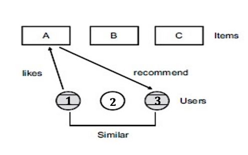
18

profiles to infer their degree of similarity. Finally, it can recommend users music with the music

in their similar users’ profiles.

 Celma (2009) provides a detailed discussion of collaborative filtering methods for

music recommendation based on real-world examples from the music field. In Celma’s work,

Memory-based CF systems handles two types of similarity relationships: item-to-item

similarity (songs or artist), and user-to-user similarity. The similarity between items can be

calculated by comparing each N-dimensional row vectors, where N is the total number of users.

The similarity between users can be calculated by comparing the corresponding M-dimensional

column vectors, where M is the total number of items.

 For vector comparison, cosine similarity and Pearson’s correlation coefficient are

popular choices. For example, Slaney and White (2007) analyze 1.5 million user ratings given

by 380,000 users from the Yahoo! music service and obtain the similarity of music piece by

comparing normalized rating vectors on the items and calculating their respective cosine

similarities.

2.5.3.1 User-based Collaborative Filtering

The user-based CF approach recommends items to the target user from his/her similar users.

For example, as seen in the Figure 2.1, in this case, user 1 and user 3 have similar music

preferences, so they are considered as a neighbor to each other. Since user 1 gives a like to

item A, the user-based CF system would recommend A to user 3. User-based CF uses users’

rating scores on items to consider their similarities and finds their k nearest neighbors. Then,

the system can make predictions based on weighted averaging score by combining all neighbors’

ratings.

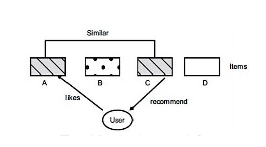
19

 Figure 2.1 User-based Collaborative Filtering Logic Flow

To make our ideas into equation, a predicted rating ′!,# for user u and an item i is calculated

by finding ! , the set of k nearest neighbors according to their rating preference with u, and

combine their ratings for item i (Konstan et al., 1997):

Where $,# denotes the rating of user g given to item i, ̅! is the average rating of user u, and

sim(u,j) is a weighting factor that corresponds to the similarity to the neighboring users.

2.5.3.2 Item-based Collaborative Filtering

The item-based CF approach recommends items by checking similarities between the items

that are already associated with the user. For example, as seen in the Figure 2.2, in this case,

item A and item C are similar, so they are considered as a neighbor to each other. Since the

user gives a like to item A, the item-based CF system would recommend C to the user. Item-

20

based CF analyzes a set of items that the target user has already evaluated to calculate the

similarities between all items and the target item. Then, the system can make predictions for

target items by comparing the user’s previous preferences on the set.

 Figure 2.2 Item-based Collaborative Filtering Logic Flow

While user-based CF identifies neighboring users by examining the rows of the user-item

matrix, item-based CF operates on the columns to find similar items. Predictions ′!,# are then

made by finding the set of k most similar item to i that have been rated by u and combining the

ratings. Since the number of rated items from each user is usually smaller than the total number

of items, item-to-item similarities can be pre-calculated and cached. In many real-world

recommender systems, item-based CF is thus chosen over user-based CF for performance

reasons (Linden et al., 2003). For determining nearest neighbors (kNNs), in both user-based

and item-based CF, cosine similarity or “cosine-like measure” are utilized (Nanopoulos et al.,

2009).

21

2.5.4 Model-based Collaborative Filtering

There are many model-based approaches to collaborative filtering, in which some are based on

Linear Algebra, such as Matrix Factorization, Principal component analysis (PCA), and

Eigenvectors; some others use techniques derived from Artificial Intelligence, such as Bayes

methods, Latent Classes, and Neural Networks; some others are based on clustering (Drineas

et al., 2002). Compared with memory-based methods, model-based algorithms are usually

preforming faster at query time, although they might need expensive learning and updating

phases. In our thesis, we focus on the Matrix Factorization-based methods.

2.5.4.1 Matrix Factorization-based Collaborative Filtering

Model-based CF methods that build upon latent factors representation are obtained by learning

factorization models of the rating matrix, e.g., (Hofmann, 2004), (Koren et al., 2009). Compare

with memory-based CF methods, matrix factorization-based CF have a few advantages,

including higher accuracy, shorter processing time since they avoid the massive calculations

directly on the rating matrix like kNN methods, and creates more explicit and compact

representations. The results of the KDD-Cup 2011 competition shows that matrix factorization

methods can significantly improve prediction accuracy in the music field (Dror et al., 2011).

 The assumption under the matrix factorization-based CF is that the observed ratings are

the result of a number of latent factors of user characteristics (e.g., preference or taste,

“personality”) and item characteristics (e.g., genre, mood, instrumentation). The purpose of

matrix factorization is trying to estimate those hidden parameters from users’ ratings. These

parameters should explain the observed ratings by characterizing both users and items in an ℓ-

dimensional space of factors. These computations derived factors basically describe the

variance in the rating data and may not be human interpretable (Ricci and Shapira, 2015).

22

 In the matrix factorization model, the rating matrix R can be decomposed into two

matrices W and H such that R = WH, where W relates to users and H to items. In the latent

space, both users and items are represented as ℓ-dimensional vectors. Each user u is represented

as a vector ! = ℓ , and each item i as a vector ℎ# = ℓ . W = [ & … ' ]( and H = [ℎ& … ℎ' ](

are thus f × ℓ and ℓ × n matrices respectively. Entries in ! and ℎ# measure the relatedness to

the corresponding latent factor. These entries can be negative. The number of latent factors is

chosen such that ℓ ≪ , , which yields a significant decrease in memory consumption in

comparison to memory-based CF. Also rating prediction is much more efficient once the model

has been trained by simply calculating the inner product ′!,# = ! ( ℎ# . More generally, after

learning the factor model from the given ratings, the complete matrix ) = contains all

ratings predictions for all user-item pairs.

2.5.5 Users’ Interactions with Recommender Systems

Other research studies explore users’ interaction with their recommender systems. Pohle et al.

(2007) present a user interface that allows users to choose musical concepts tags they extracted

from last.fm [7], and recommend them music match with the concepts tags they choose. Knees

and Widmer (2008) present an approach to adapt user preferences on music by incorporating

relevance feedback. Mesnage et al. (2011) build a social music recommender system by

investigating Facebook, and recommend music based on users’ friend relationships and their

interactions with other users.

23

2.6 Conclusion

We have gone through the state-of-the-art methods of music content-based, music context-

based, and user context-based in music recommendation tasks. In contrast to the content-based

and text-based approaches reviewed in sections 3 and 4, collaborative filtering techniques used

in user context-based methods could outperform the previous two methods in today’s industry

since they do not require any additional metadata and calculations that related to the music

pieces themselves. Due to the nature of rating matrix, similarities can be directly calculated

without correlating the occurrence of metadata with actual items. However, these CF

approaches are sensitive to factors such as popularity biases and data sparsity.

 In the following section, we discuss the process of our dataset preparations, and

introduce the CF models will be used in our experiment.

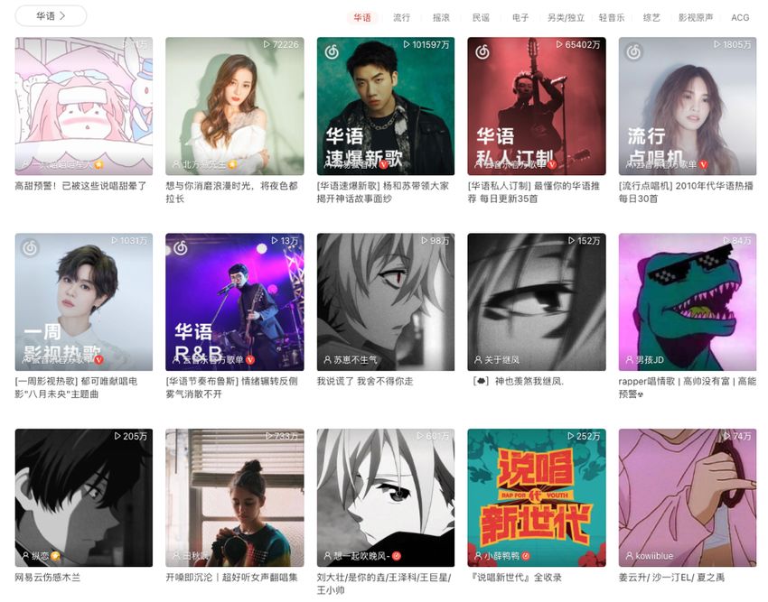
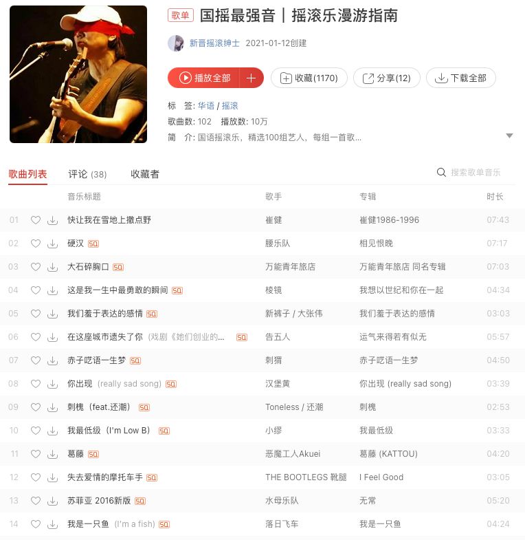
24

3. Methodology

3.1 Dataset

The raw dataset was crawled from NetEase Cloud Music [9], one of the largest music streaming

platforms in China, with over 300 million users and a music database containing over 10 million

songs. On this platform, users can search and listen to a large number of songs. When a user

encounters a song he likes, he/she can click the “Like” button and add it to his/her playlist.

Users can add tags to their playlists to illustrate the style of the songs in the playlist, such as

"Mandarin", "Popular", "Electronic", etc. Each user can create multiple playlists, and at the

same time set the playlists to be public so that they can be accessed by other users. Accessing

the playlists of other users is the major way for users to explore music. On the homepage of the

platform, popular playlists are displayed for other users to access. Users can also subscribe

other users' playlists to get the latest music trends. The homepage interface of NetEase Cloud

Music is shown on Figure 3.1. The interface of a single playlist is shown on Figure 3.2.

 Interestingly, NetEase Cloud Music has already provided users with a "Daily Song

Recommendation" playlist function. According to the user's behavior, this playlist will

automatically generate 20 songs that the user may like every day. The company may use more

indicators to help them measure users' behavior, such as users remove an item from the playlist,

user skipping a song, and the time they spent on a particular page and the number of clicks.

However, we cannot access this part of the information, nor can it be obtained through web

crawling. The only information we can obtain is the playlist of each user and the songs

contained in it. Since we want to focus on Chinese Music, we only crawl the playlists that

contain Mandarin tags.

25

Figure 3.1 Interface of NetEase Cloud Music’s Homepage

 Figure 3.2 Interface of a single playlist

26

 Our dataset contains over 50,000 public playlists contain Mandarin tag of

corresponding users and more than 200,000 songs. The format is in JSON, and the size of our

file playlist.detail.all.json is 16.08 Gigabyte. In addition to the metadata of the playlist, each

playlist also includes all the tracks in the playlist and their metadata. The sample format of each

playlist and each song are listed in the Appendix A and Appendix B.

3.1.1 Parse Dataset

Since the raw dataset contains too many playlists and songs, it is difficult to process this amount

of information on a personal computer. Also, some of the playlists in the dataset only have few

songs, which cause the problem of data sparsity. So, we need to parse the raw dataset.

 We find that the playlists with more subscribers, in general, have more songs. Those

users are considered active users of the platform. So, we only take those playlists with more

than 100 subscribers (subscribedCount > 100). The total number of playlists that fit the

requirement is 1076, containing 49774 songs. Also, the raw dataset contains too much

information, including createTime, updateTime, description, URLs and many tags, etc. This

part of the information is not very helpful to our research, so we decided to extract only a few

of the most important elements and convert the raw dataset into a simplified dataset. For each

playlist, only four dimensions of the information including playlist name, category, playlist id,

and the number of subscribers is extracted. For each song, only four dimensions of the

information including song id, song title, singer, and song popularity is extracted. For each

playlist and the songs contained in it, we organize them into the following Table 3.1:

27

 Table 3.1 Sample format of a Playlist

 Playlist ##流行,华语##57364826##3572

 Track 1 28643203::花房姑娘::崔健::57.0

 Track 2 407007442::末班车::信::46.0

 Track 3 33162226::友情岁月::李克勤::85.0

 Track 4 28387594::无赖::林忆莲::74.0

 Track … ......

3.1.2 Format Dataset for Recommender System

Users’ rating to an item is an explicit feedback. For some datasets, they contain such

information, so those rating could be used in the matrix. Nonetheless, for other datasets, they

do not contain rating information, just as the dataset in our experiment. In this case, we need to

use users’ implicit feedback as their rating information. For example, users’ browsing, or

purchase history could be used as their rating.

 Since the playlist is a collection behavior, which shows the user's interest in the songs

in the playlist, the songs in each user's playlist can be regarded as a positive feedback of the

user for the songs in the playlist. However, users’ negative feedback on songs cannot be directly

reflected in the user’s collection behavior. This is determined by user’s behavior when

consuming music. When they dislike a song, the usual behavior is to skip it. Although NetEase

Cloud Music provides users with the function of disliking songs, which is a clear negative

feedback, users usually choose to skip the current song instead of clicking the dislike button

for the song they dislike, resulting in a small amount of data in this part. Also, the data of users'

dislike songs are not displayed on the playlist page and cannot be obtained through crawlers.

28

 Based on these considerations, we assume that the songs that are not collected by users

reflect their dislike of these songs to a certain extent. Although it is a bit arbitrary, we decided

to directly sample the songs outside of each user’s playlist as a negative feedback for them.

This creates a binary matrix, where “1” stands for “rated and like”, and “0” for “dislike”.

Although songs may not be selected into the playlist is because users have not listened to these

songs, we believe this is the best solution to approach our dataset based on our knowledge. The

entire experiment was performed under this assumption, which could be one of our limitation,

and further discussion is in the section 4.

 Figure 3.3 Sample MovieLens dataset format

For mainstream python recommendation system frameworks, the most basic data format

supported is the MovieLens dataset [2] ,and its data format is user-item-rating-timestamp. Its

format is shown in Figure 3.3. In order to use the framework, we decide to process our data

into the same format. For rating information, we set the positive feedback to score 1.0, and the

negative feedback to 0.0. For timestamp information, since our data do not have this part of

information, and it actually have no effect on our algorithms, we simply give them the same

value 1300000. Since we find the average items contained in all the playlists is 150 items, we

29

construct 150 negative sample for each user and generate the files music_format_neg.txt. Then

we merge the data of music_format_neg.txt into music_format.txt to get the final model training

data music_format_full.txt. In the modeling process, we randomly split the train set at the ratio

of 75%:25%, and take 25% as the test set. The final data format is as the following Table 3.2:

 Table 3.2 Sample format of our dataset following MovieLens

 user_id, song_id, score, time_stamp

 392991828,33891487,1.0,1300000

 392991828,31168297,1.0,1300000

 392991828,101085,1.0,1300000

 392991828,407761300,1.0,1300000

 392991828,29738501,0.0,1300000

 392991828,48365894,0.0,1300000

 ......

3.2 Models

This paper uses the python library Surprise (Hug, 2020) in the modeling process of the

recommender system. Surprise is a Python library for building and analyzing rating prediction

algorithms. It was designed to closely follow the scikit-learn API.

 We use the models listed in Table 3.3 to predict the user-item ratings and we will discuss

their performance in the section 4.

30

 Table 3.3 Models used in our experiment

Category Name Description

Baseline Min Predictor A baseline algorithm predicting a

 minimum rating based on the train set.

Baseline Max Predictor A baseline algorithm predicting a

 maximum rating based on the train set.

Baseline Normal Predictor A baseline algorithm predicting a

 random rating based on the distribution

 of the train set.

Memory-based kNN Basic A basic kNN CF algorithm.

(Neighborhood-based)

Memory-based kNN with Means An improved kNN algorithm, taking the

(Neighborhood-based) mean normalization of each user into

 account.

Memory-based kNN with Z-Score An improved kNN algorithm, taking the

(Neighborhood-based) z-score normalization of each user into

 account.

Model-based Slope One A simple yet accurate CF algorithm.

Model-based SVD An algorithm to identify latent

(Matrix Factorization) semantic factors by decomposing

 matrix.

Model-based SVD++ An improved SVD algorithm, taking

(Matrix Factorization) implicit ratings into account.

31

3.2.1 Notation Schema

Our notation schema is listed in following Table 3.4.

 Table 3.4 Notation Schema

 R the set of all ratings.

 Rtrain , Rtrain , Rˆ the training set, the test set, and the set of predicted ratings.
 U the set of all users. u and v denote users.
 I the set of all items. i and j denote items.
 Ui the set of all users that have rated item i.

 U ij the set of all users that have rated both items i and j.
 Iu the set of all items rated by user u.
 I uv the set of all items rated by both users u and v.
 rui the true rating of user u for item i.
 rˆui the estimated rating of user u for item i.

 bui the baseline rating of user u for item i.
 u the mean of all ratings.
 uu the mean of all ratings given by user u.
 ui the mean of all ratings given to item i.

 su the standard deviation of all ratings given by user u.

 si the standard deviation of all ratings given to item i.

 N ik (u ) the k nearest neighbors of user u that have rated item i.

 N uk (i ) the k nearest neighbors of item i that are rated by user u.

32

3.2.2 Baselines

We propose three baseline models to evaluate the effectiveness of all other models. The idea

here is our algorithms must at least perform better than our baselines to prove they are doing a

predictive job. The Min Predictor would always output 0, which means dislike; and the Max

Predictor would always output 1, which means like. The Normal Predictor predicts a random

number based on the normal distribution of our training set, which would be a fraction number

between 0 and 1.

3.2.2.1 Min Predictor

Min Predictor predicts a minimum rating based on the train set, which is 0 in our dataset.

 ̂!# = min !#

3.2.2.2 Max Predictor

Max Predictor predicts a maximum rating based on the train set, which is 1 in our dataset.

 ̂!# = max !#

3.2.2.3 Normal Predictor

The Normal Predictor Baseline algorithm predicts a random rating based on the distribution of

the train set. The prediction ̂!# is generated from a normal distribution N (uˆ, sˆ 2 ) where < and

 < are estimated from the training data using Maximum Likelihood Estimation.

 1
 µˆ = å rui
 | Rtrain | rui ÎRtrain

33

 (rui - µˆ )2
 sˆ = å
 rui ÎRtrain | Rtrain |

3.2.3 kNN-based Models

The k-Nearest-Neighbors (kNN) is a non-parametric classification and case-based learning

method, which keeps all the training data for classification (Ricci and Shapira, 2015). It is

simple but effective in many cases. For a user u to be classified, its k nearest neighbors are

retrieved, and this forms neighborhoods of u. The kNN-based algorithm automates the general

principles of word-of-mouth, in which people consider and rely on the opinions of other like-

minded people to evaluate items. It mainly including user-based and item-based two directions.

 In the user-based CF scenario, when user A needs personalized recommendations, the

system would first find other users who have similar interests with A, and then recommend

those items that those user likes but that the user A has never known. The user-based CF

algorithm mainly includes two steps: First, investigate the set of users with similar interests to

the target users, and find its k nearest neighbors; Second, find items in those users’ collections

and not in the collection of the target user, and recommend them to the target users.

 The item-based CF is the most widely used algorithm in the industry, recommending

similar items to the users they previously liked. The item-based collaborative filtering

algorithm mainly includes two steps: First, calculate the similarity between all items in the set

with the target item, and find its k nearest neighbors; Second, generate recommendations for

the user based on the similarity of items.

 In all the kNN algorithms performed in our experiment, we set their k value equals 40.

34

3.2.3.1 kNN Basic

A basic form of kNN algorithm. The prediction ̂!# is set as:

 å sim(u, v) × rvi
 vÎN ik ( u )
 User-based: rˆui =
 å sim(u, v)
 vÎNik ( u )

 å sim(i, j ) × ruj
 jÎNuk ( i )
 Item-based: rˆui =
 å sim(i, j )
 jÎNuk ( i )

3.2.3.2 kNN With Normalization

Normalization is the process of adjusting values measured on a different scale to a common

scale. It compensates for the difference in users' behavior by adjusting the rating scale, and

make the range comparable or same with other users' ratings. Without normalization, our data

would be unscaled and hence highly intricate to calculate and compare with other parameters

(Pandey et al., 2017). There are many normalization techniques, including feature scaling,

coefficient of variation, studentized residual, standard score (Z-Score), etc. In this thesis, we

use Mean-centering and Z-Score to Normalize (Breese et al., 1998).

3.2.3.2.1 kNN with Means

kNN with Means is an improved kNN algorithm, in which the mean ratings of each user or item

are considered. The idea of centering the mean is to determine whether a rating is positive or

negative by comparing it with the mean rating. In user-based CF, the raw rating !# is

35

transformed into ℎ( !# ) by subtracting the average of the rating ?! to !# . In item-based CF, the

ℎ( !# ) is done in the similar manner.

 ℎ( !# ) = !# − ?!

In our experiment, the prediction ̂!# is set as:

 å sim(u, v) × (rvi - µv )
 vÎNik ( u )
 rˆui = µu +
 å sim(u, v)
 vÎNik ( u )
 User-based:

 å sim(i, j ) × (ruj - µ j )
 jÎNuk ( i )
 rˆui = µi +
 å sim(i, j )
 jÎNuk ( i )
 Item-based:

3.2.3.2.2 kNN with Z-Score

kNN with Z-Score is an improved kNN algorithm, considering the Z-Score normalization of

each user or item. The Z-Score normalized each score to its number of standard deviations that

it is distant from the mean score. While mean-centering eliminates the drift caused by the

different perceptions of the average rating, Z-Score also takes into account the difference in

each individual scales. In user-based CF, ℎ( !# ) equals to mean-centered !# divided by the

standard deviation ! . In item-based, the ℎ( !# ) is done in the similar manner.

 !# − ?!
 ℎ( !# ) =
 !

36

In our experiment, the prediction ̂!# is set as:

 å sim(u, v) × (rvi - µv ) / s v
 vÎNik ( u )
 rˆui = µu + s u
 å sim(u, v)
 vÎNik ( u )
 User-based:

 å sim(i, j ) × (ruj - µ j ) / s j
 jÎNuk ( i )
 rˆui = µi + s i
 å sim(i, j )
 jÎNuk ( i )
 Item-based:

3.2.3.3 Similarity Metrics for kNN Models

The similarity weights play an important role in neighborhood-based CF methods. They

provide different methods to give these neighbors more or less weight in the prediction.

 For kNN Basic, kNN with Means, and kNN with Z-Score, we use the following three

metrics in Table 3.5 to calculate their similarity for both user-based and item-based methods.

 Table 3.5 Similarity Metrics for kNN Models

 Cosine Similarity Calculate the Cosine Similarity for both user-

 based and item-based kNN models.

 Mean Squared Difference (MSD) Calculate the Mean Squared Difference for both

 user-based and item-based kNN models.

 Pearson Correlation Coefficient Calculate the Pearson Correlation Coefficient for

 both user-based and item-based kNN models.

37

3.2.3.3.1 Cosine Similarity

Cosine similarity is one of the most popular metrics used in Information Retrieval. It treats

objects as vectors in an N-dimensional vector space. In the following equation, cosine similarity

investigates the angle between two vectors, item i and item j. !,# is the rating of item i given

by user u. !,* is the rating of item j by user u. n is the total number of all ratings to item i and

item j (Billsus and Pazzani, 1998).

 ⃗ ⋅ ⃗ ∑,!-& !,# !,*
 ( , ) = ( ⃗, ⃗) = =
 ‖ ⃗‖+ ‖ ⃗‖+
 M∑,!-& !,# + M∑,!-& !,* +

Two vectors are considered similar if the angle between them is small. When the angle reaches

0 digress, sim(i,j) = 1, indicating we can regard them as identical. When the angle reaches 180

digress, sim(i,j) = -1, indicating we can regard them as opposite. If the angle is 90 degrees,

sim(i,j) = 0, meaning the two vectors are irrelevant. In our cases, sim(i,j) ranges from 0 to 1.

In our experiment, we calculate the cosine similarity between all pairs of users and items. The

cosine similarity for users is defined as:

 år
 iÎIuv
 ui × rvi
 cosine_sim(u, v)=
 år
 iÎIuv
 2
 ui × år
 iÎI uv
 2
 vi

38

The cosine similarity for items is defined as:

 år
 uÎUij
 ui × ruj
 cosine_sim(i, j)=
 år
 uÎUij
 2
 ui × år
 uÎUij
 2
 uj

3.2.3.3.2 Mean Squared Difference

Mean Squared Difference (MSD) evaluates the similarity between two users u and v as the

inverse of the average squared difference between the rating given by u and v on the same

items (Shardanand and Maes, 1995).

We calculate the Mean Squared Difference similarity between all pairs of users or items. The

MSD for users is defined as:

 1
 msd_sim(u, v)=
 1
 × å (rui - rvi ) 2 +1
 | I uv | iÎIuv

The MSD for items is defined as:

 1
 msd_sim(i, j ) =
 1
 × å (rui - ruj )2 +1
 | U ij | uÎUij

39

3.2.3.3.3 Pearson Correlation Coefficient

 Pearson correlation coefficient is one popular method used in collaborative filtering

tasks. It measures the tendency of two number series, paired up one-to-one and move together

(Deshpande and Karypis, 2004). The Pearson correlation coefficient can be considered as an

improved cosine similarity with mean-centered (Ricci and Shapira, 2015). As in the following

equation, it measures the linear correlation between two vectors item i and item j.

 ⟨ !,# − # , !,* − * ⟩ ∑,!-&( !,# − # )( !,* − * )
 ( , ) = =
 Q !,# − # QQ !,* − * Q R∑,!-&( !,# − # )+ R∑,!-&( !,* − * )+

n is the total number of all ratings given to i and j. !,# is the rating of item i given by user u,

 !,* is the rating of item j given by user u. # is the average rating of item i for all the co-rated

users, and * is the average rating of item j for all the co-rated users. When two the vectors are

in a high level of similar tendency, sim(i,j) is close to 1; when two vectors are in a low level of

similar tendency, sim(i,j) is close to 0. When two vectors have an opposite tendency, sim(i,j) is

-1. In our cases, sim(i,j) ranges from 0 to 1.