Use of Topographic Models for Mapping Soil Properties and Processes - MDPI
←
→
Page content transcription
If your browser does not render page correctly, please read the page content below
Review
Use of Topographic Models for Mapping Soil
Properties and Processes
Xia Li 1, * , Gregory W. McCarty 1, *, Ling Du 1 and Sangchul Lee 1,2
 1    Hydrology and Remote Sensing Laboratory, USDA-ARS, Beltsville, MD 20705, USA;
      Ling.Du@usda.gov (L.D.); sangchul.lee@usda.gov (S.L.)
 2    Department of Environmental Sciences and Technology, University of Maryland, College Park, MD 20742, USA
 *    Correspondence: xia.li@usda.gov (X.L.); greg.mccarty@usda.gov (G.W.M.); Tel.: +1-(301)-504-7401 (G.W.M.);
      Fax: +1-(301)-504-8931 (G.W.M.)

 Received: 3 April 2020; Accepted: 12 May 2020; Published: 15 May 2020

 Abstract: Landscape topography is an important driver of landscape distributions of soil properties
 and processes due to its impacts on gravity-driven overland and intrasoil lateral transport of water
 and nutrients. Rapid advancements in aerial, space, and geographic technologies have led to large
 scale availability of digital elevation models (DEMs), which have proven beneficial in a wide range of
 applications by providing detailed topographic information. In this report, we presented a summary
 of recent topography-based soil studies and reviewed five main groups of topographic models in
 geospatial analyses widely used for soil sciences. We then compared performances of two types of
 topography-based models—topographic principal component regression (TPCR) and TPCR-kriging
 (TPCR-Kr)—to ordinary kriging (OKr) models in mapping spatial patterns of soil organic carbon (SOC)
 density and redistribution (SR) rate. The TPCR and OKr models were calibrated at an agricultural
 field site that has been intensively sampled, and the TPCR and TPCR-Kr models were evaluated
 at another field of interest with two sampling transects. High-resolution topographic variables
 generated from light detection and ranging (LiDAR)-derived DEMs were used as inputs for the TPCR
 model building. Both TPCR and OKr models provided satisfactory results on SOC density and SR rate
 estimations during model calibration. The TPCR models successfully extrapolated soil parameters
 outside of the area in which the model was developed but tended to underestimate the range of
 observations. The TPCR-Kr models increased the accuracies of estimations due to the inclusion of
 residual kriging calculated from observations of transects for local correction. The results suggest
 that even with low sample intensives, the TPCR-Kr models can reduce estimation variances and
 provide higher accuracy than the TPCR models. The case study demonstrated the feasibility of using
 a combination of linear regression and spatial correlation analysis to localize a topographic model
 and to improve the accuracy of soil property predictions in different regions.

 Keywords: landscape topography; LiDAR-derived DEM; soil organic carbon; soil redistribution;
 ordinary kriging; topographic principal component regression kriging

1. Introduction
     A study of landscape topography is an assessment of the current terrain features and a
representation of the landforms. Because topography reflects elevation changes within detailed
landform features over a region, it can significantly impact the geomorphological, hydrological, and
biological processes on the earth [1]. The spatial variability of topographic features (e.g., relief, slope,
and curvatures) controls gravity-driven overland and intrasoil lateral transport of water and nutrients,
and impacts soil hydrological regimes, climate, and vegetation types [2].

Soil Syst. 2020, 4, 32; doi:10.3390/soilsystems4020032                         www.mdpi.com/journal/soilsystems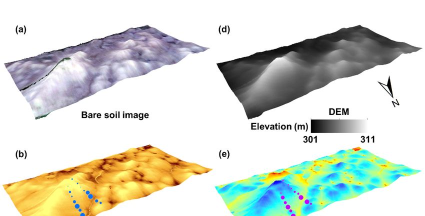
Soil Syst. 2020, 4, 32                                                                              2 of 19

      Topography has been widely used in soil science, with topographic information being derived from
multiple sources. Before the 1990s, the main source was geographic maps [1]. Using geomorphometric
techniques, the topographic metrics, such as slope gradient and curvatures, were produced manually
and applied to investigate spatial variability in soil properties and to produce soil maps [3–5]. With the
development of computer and geophysical technologies, more and more scientists have used digital
elevation models (DEMs) derived from photogrammetry to calculate topographic metrics. A series of
topographic metrics were developed due to the improvement of mathematical theory and physical
understanding of topographic surface features.
      The objective of this study is to provide an overview of topographic models for predictions of soil
properties and processes. The prerequisites for developing an effective topography-based soil property
model are that (1) the impacts of topography on soil properties can be investigated through a small set
of samplings over a small scale, and (2) strong statistical correlations exist between topography and
soil properties. Therefore, this review begins with an introduction of topography-based soil studies,
following investigations of topographic metrics that are important for soil models and five main groups
of topographic models. The last section presents a case study to assess the efficiency of high-resolution
topography-based models for mapping soil organic carbon (SOC) and redistribution.

2. Topographic Metrics for Soil Studies
     Various studies have demonstrated the utility of including topographic metrics in soil models to
better simulate spatial patterns of soil properties and processes [6–15]. Topographic metrics quantify
characteristics of the topographic features. According to the calculation methods, topographic metrics
can be divided into primary and secondary (combined) metrics [16]. Primary metrics are directly
calculated from elevation, such as slope, aspect, and curvatures. The metrics are further grouped into
local and nonlocal because of the spatial scope [1]. Local metrics describe the surface geometry at a
given point, whereas nonlocal metrics consider relative positions of a selected location. Secondary or
combined metrics combine primary metrics and usually describe spatial variability in specific processes
such as water content distribution and soil erosion potential. Table 1 lists definitions of topographic
metrics that were reported to impact soil movement and properties.
Soil Syst. 2020, 4, 32                                                                                          3 of 19

                                 Table 1. Definitions of selected topographic metrics.

                 Category                          Variable                               Definition
                                               Altitude, H (m)                            Elevation
                                                                          An angular measure of the relation between
                                          Slope gradient, G (radian)
                            Local                                          a tangent plane and a horizontal plane
                         topographic    Profile curvature, P_Cur (m−1 )    Slope change rates in the vertical plane
                           metrics      Plan curvature, Pl_Cur (m−1 )          Curvature in a horizontal plane
                                                                          Upslope area contributing runoff to a given
                                           Catchment area, CA (m2 )
                                                                                  point on the land surface
                                         Upslope slope, UpSl (radian)           Mean slope of upslope area
     Primary                             Downslope index, DI (radian)        Head differences along a flow path
     metrics                                                                Maximum distance of water flow to a
                                          Flow path length, FPL (m)
                                                                                 location in the catchment
                           Nonlocal                                       Land area that contributes surface water to
                         topographic     Flow accumulation, FA (m2 )
                                                                              an area in which water accumulates
                           metrics                                         Elevation difference between the highest
                                          Topographic relief, TR (m)
                                                                               point in an area and a given point
                                                                                Angular measure describing the
                                          Topographic openness, TO
                                                                            relationship between surface relief and
                                                  (radian)
                                                                                       horizontal distance
                                          Topographic wetness index,        Frequencies and duration of saturated
                                                    TWI                                   conditions
    Secondary                              Stream power index, SPI             Erosive power of overland flow
     metrics
                                                                            Factor that considers slope length and
                                            Length–slope factor, LS
                                                                                 steepness effects on erosion

2.1. Primary Metrics

2.1.1. Local Topographic Metrics
     Slope gradient (G), profile curvature (P_Cur), and plan curvature (Pl_Cur) can control
gravity-driven overland and intrasoil lateral transport of water and nutrients. G suggests the steepness
of a location, which can directly influence water infiltration and soil erosion [17,18]. Compared to
relatively flat areas, steeper areas tend to have less infiltration and higher erosion possibilities,
decreasing soil moisture and transporting fine soil particles with high SOC content from the areas [2,7].
Furthermore, most of the soil-forming processes (e.g., carbonate dynamics, clay illuviation, and so
on) are more efficient on more gently-sloping land surfaces [19,20]. P_Cur is parallel to the direction
of maximum slope, and therefore affects soil redistribution and SOC distribution patterns through
influencing flow acceleration and deceleration [21–23]. Pl_Cur is perpendicular to the direction of
maximum slope, which determines flow divergence and convergence [1,24,25].
     Altitude (H) impacts soil properties by affecting climate and insolation. Changes in H cause
variations in climate. Generally, decreased temperature and increased precipitation occurs in areas
with elevated altitude. Temperature and precipitation changes affect vegetation composition and
productivity, which in turn influence soil properties and water content [26].

2.1.2. Nonlocal Topographic Metrics
     Multiple nonlocal topographic metrics can significantly impact the gravity-driven processes,
including upslope slope (UpSl), downslope index (DI), and topographic relief (TR). UpSl reflects
the steepness of the upslope contributing areas, which is positively related to overland flow
velocities [16,25,27]. DI is also a slope gradient associated metric, but it considers the water balance
between the water from a specific upslope contributing area and a downslope area [28]. Therefore, this
metric is highly correlated with groundwater gradients and soil water content [28,29]. High values of
TR reflect large differences between the highest and the target locations, and thus high overland flow
velocities are usually observed with potentials for large downslope soil transport [7,8,30].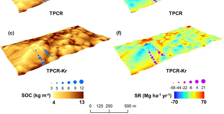
Soil Syst. 2020, 4, 32                                                                             4 of 19

     Catchment area (CA), flow path length (FPL), flow accumulation (FA), and topographic openness
(TO) affect soil properties through influencing soil hydrological regimes, causing variability in soil
C decomposition, denitrification, and nitrification processes. Increased CA enhances the chance for
sediment deposition, changing the soil C stocks [31]. Longer FPL decreases overland flow velocity
and increases soil infiltration and erosion [32–34]. This metric is widely used in soil erosion models
because it reflects soil loss under flow divergence and convergence conditions [35,36]. FA impacts
water conditions in the soil, which is positively related to flow volume and soil water content [37,38].
TO exhibits convex (high positive TO and low negative TO values) and concave (low positive TO and
high negative TO values) landforms [39]. Therefore, soil water contents are likely high in locations with
low positive TO values, providing suitable anaerobic environments for denitrification but impeding
aerobic C decomposition [7,8].

2.2. Secondary Metrics
      Commonly used secondary topographic metrics generally address aspects of the physics     of water
                                                                                          CA
movement on landscapes. Topographic wetness index (TWI) is calculated as TWI = ln G . This index
is widely used to reflect the spatial distribution of wetness conditions [7,40–42]. Locations with high
values of TWI have high possibilities to be wet locations. TWI has proved to be an effective index for
understanding spatial patterns of soil hydrological and geochemical properties and is significantly
correlated with soil C and N content [7,8].
      Stream power index (SPI) considers specific contributing area (CAs ), Pl_Cur (PlCur ), and G with
the equation as SPI = CAs (PlCur ) tan(G). The metric is useful for investigating potential erosive
powers of water flow [43]. The increased G and CA lead to increased water flow velocity and water
amount, and consequently enhancing water erosive power [44].
      Length-slope factor (LS) is a combination of slope length and slope gradient. There are three
major methods for LS calculation, including models developed by Moore and Nieber [45], Desmet and
Gover [46], and Wischmeier and Smith [47]. Increased slope length usually increases the soil loss per
unit area because of a greater runoff accumulation on a longer slope length, whereas slope steepness
increases also stimulate soil loss.
      Large collinearities often exist between these topographic metrics (Table 1) for a given landscape,
with two main causes for the correlations—one being these metrics quantify the properties of a
self-organized landscape whose properties would be expected to be correlated, and another being that
various metrics are derived from mathematical equations containing common elements that induce
correlations between the resulting metrics. Principal component analysis (PCA) is a common approach
to generate sets of orthogonal factors from correlated metrics and thereby reduce the dimension of
parameters. These PCA factors, in turn, can be used as a set of orthogonal parameters in prediction
models. This is the approach that Li et al. [6–9] used in developing more robust topographic models
using information contained within 15 topographic metrics with reduced dimensionality. Interestingly,
the resulting PCA factors were combinations of local, nonlocal, and secondary metrics reflecting the
connectedness of landscape network processes and information flow.

3. Soil-Landscape Models for Soil Property Mapping
      Along with the development in computer, aerial, space, and geographic techniques, increasing
attention has been paid to soil-landscape modeling to predict spatial patterns of soil morphological,
chemical, and physical properties. Recently, detailed large-scale topographic information can be derived
due to the increased availability of high-resolution DEMs, providing a possibility for regional-scale
soil property predictions based on topography-based models. There are five main groups of models
with strong application in landscape modeling.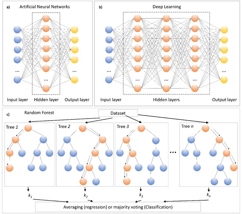
Soil Syst. 2020, 4, 32                                                                                  5 of 19

3.1. Geostatistical Models
      Geostatistical models deal mainly with spatial data and explain spatial autocorrelation using
interpolator. Kriging is a representative geostatistical model with a form of weighted averages
generating an estimate from a scattered set of measured values. One limitation of kriging is that
it is an interpolation technique, and thus predictions are only valid for regions that have multiple
measured values. Estimation in a finite domain can provide too much weight to points, leading to
biased estimations [48,49]. In 1980, Burgess and Webster first introduced ordinary kriging (OKr) to map
soil textures [50]. Since then, a large body of literature has formed that is based on application of OKr
to interpolate soil properties, such as fertility [9], salinity [51], soil water content [52], and infiltration
rates [49]. However, OKr fails to consider the knowledge of soil materials and landscape. The efficiency
of the prediction usually depends on large samplings at the field scale [49].
      To overcome the above OKr limitations, several methods, such as regression kriging (RKr),
cokriging (CKr), and kriging with external drift (KED), have been developed to incorporate ancillary
data into the OKr model. Combining OKr with multiple linear regression (MLR), RKr spatially
interpolates the residuals from a MLR model using kriging and adds the interpolation to the prediction
to improve the performance of the MLR model. In soil science applications, various studies have
used this method for analyzing spatial patterns of soil horizon thickness [13,14], soil structures [13,14],
soil water availability [53], cation exchange capacity [15,54], soil C content [55,56], and hydraulic
properties [57,58]. The CKr model takes advantage of correlations between the investigated variable
and other easily estimated variables. KED uses external ancillary variables to represent the trend of soil
properties. CKr and KED models have also been employed in investigating soil physical and chemical
characteristics [12–15]. Several studies have reported that performances of topography-based CKr and
KED models are better than OKr models in soil property estimation in areas that are strongly impacted
by landscape [49,59].

3.2. Logic Models
     Fuzzy Logic (FL) is a widely used logical method with soil mapping applications. It is an extension
of Boolean logic to express the degree of similarity to a classification type using membership values
ranging from 0 (non-membership value) to 1 (membership value) [60]. Because soils are continuums
in both geographic and attribute spaces, allowing partial truth of independent variables is especially
useful and provides sufficient information about soil properties when compared with the traditional
setting of 0 or 1 [61,62]. Topography-based FL has been applied in soil mapping to improve soil
taxonomic classification [63–67]. Several studies also used the model to study spatial patterns of soil
horizonation [64,68,69], predict soil texture [68,70], and classify soil vulnerability [71].

3.3. Decision Tree Analysis
      As a divisive supervised classification, decision tree analysis (DTA) successively partitions a
dataset into increasingly homogenous subsets. Rules applied to split the data area can be either
categorical, such as geographical unit number and soil unit, or continuous, such as elevation and
slope [72,73]. A useful rule can decrease impurity of the dataset. Therefore, by developing a set of
rules from training data, the DTA can be applied to regions with the same inputs to predict the target
variable. This method is useful for capturing nonadditive and nonlinear relationships, and is easier to
interpret than standard statistical approaches because the output is based on a set of nominal and/or
continuous rules [74].
      In accordance with different splitting methods, DTA can be divided into two classes:
(1) homogeneous decision tree and (2) hybrid decision tree. The homogeneous decision tree uses a single
algorithm in each partition [75]. One representative homogeneous decision tree is the classification
and regression trees (CART) algorithm. A topography-based CART can be applied to derive
efficient categorical information, such as soil taxonomic classes and soil drainage classification [76–79].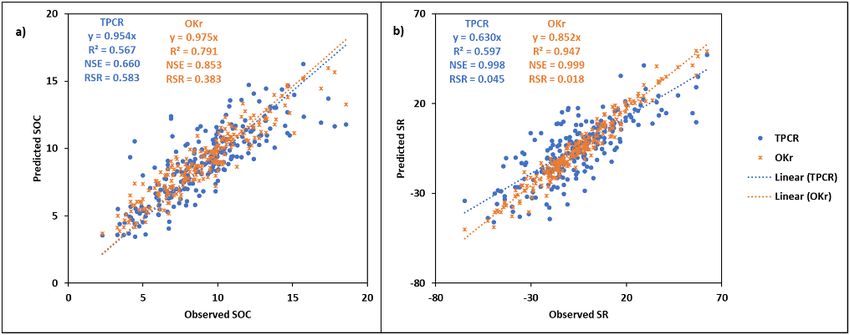
Soil Syst. 2020, 4, 32                                                                              6 of 19

Researchers have also successfully used topography-based CART for quantitatively predicting soil
properties such as soil cation exchange and water retention [15,80]. The hybrid decision tree may
use different splitting algorithms at different points. Friedl and Brodley [75] found that this method
demonstrated the highest accuracy in classification when comparing different DTA methods.

3.4. Standard Statistical Methods
      Statistical methods, including multiple linear regression (MLR) and discriminant analysis (DA),
are widely used to quantify impacts of the landscape on soil properties and to generate soil maps.
MLR uses two or more independent variables to simulate a target soil property or process through
fitting to a linear equation. The topography-based MLR models do demonstrate, in a quantitative
manner, the fact that terrain analysis can be applied to predict spatial patterns of soil physical and
chemical properties over large spatial scales [6–12]. MLR has also combined with other methods to
improve the efficiency of prediction. For example, Li et al. [7] developed topography-based models
based on a principal component regression (PCR) combining principal component analysis and MLR
to predict soil redistribution processes and SOC content. Results suggested that the PCR outperformed
regular MLR with a more robust prediction over different spatial scales.
      DA is a type of supervised classification using categorical criteria to assign an independent
variable to the most likely group. The main idea of DA is to develop a set of decision rules on the
basis of the measured data using a certain category variable of interest and several auxiliary variables.
With establishment of rules, the variable of interest in areas where the auxiliary variables are available
can be predicted. This method has been proposed to generate soil texture maps using topographic
metrics and other ancillary variables [81,82]. Several studies also demonstrated the feasibility of using
the DA to predict soil drainage classes due to its high correlations with topography and soil electrical
conductivity [83,84].

3.5. Advanced Statistical Methods
     Machine learning (ML) is a rapidly developing approach to data analysis that is based on ideas that
computers can learn from data, identify trends, and make decisions with limited human intervention.
Successful ML methods have several common advantages. ML methods only need a limited number of
user-defined parameters. They are able to deal with nonlinear relationships, predict quantitative and
category variables, reduce overfitting, and remain robust regardless of outliers [85]. Due to advances
in computing power and data availability, increasingly researchers have applied ML in soil mapping
applications. Three widely used ML methods on soil property predictions are artificial neural networks
(ANNs), deep learning (DL), and random forest (RF) (Figure 1).
     ANNs consist of one input layer, one output layer, and one layer of hidden interconnected units
(neurons) connecting input and output layers (Figure 1a). With this method, the outputs are related to
the input variables, developing linked algorithms of the ANNs model. All links between the input
and hidden layers compose the input weight matrix, and links between hidden and output layers
are the output weight matrix. The weights can be adjusted iteratively on the basis of the training
dataset. Including topographic information and other environmental variables, this method has been
successfully applied to identify categorical characters, such as soil taxonomic classes and drainage
classification [79,86–89], and to predict quantitative variables including soil chemical and hydrological
properties [90–92].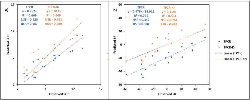
limited number of user-defined parameters. They are able to deal with nonlinear relationships,
predict quantitative and category variables, reduce overfitting, and remain robust regardless of
outliers [85]. Due to advances in computing power and data availability, increasingly researchers
have applied ML in soil mapping applications. Three widely used ML methods on soil property
predictions
Soil             are
     Syst. 2020, 4, 32artificial neural networks (ANNs), deep learning (DL), and random forest (RF) (Figure
                                                                                                      7 of 19
1).

     Figure 1.
     Figure   1. Different
                 Differentmachine
                            machinelearning
                                     learningarchitectures:
                                               architectures:
                                                            (a)(a) artificial
                                                                artificial    neural
                                                                           neural    networks,
                                                                                  networks,     (b) deep
                                                                                            (b) deep     learning,
                                                                                                     learning, and
     andrandom
     (c)  (c) random    forest.
                  forest.

     Advances in computing ability, such as innovative graphics processing units (GPUs), have enabled
the use of deep neural networks. DL is considered as an advanced ANN, which includes multi-hidden
layers instead of the single hidden layer structure in ANNs (Figure 1b). Learning through multi-layer
nonlinear transformations, DL can be used to define edges within images and perform automatic
feature extraction [93]. Two major architectures of DL are convolutional neural networks (CNNs)
and recurrent neural networks (RNNs). CNNs are based on a layer of convolving window moving
along a data array to detect features [94]. Padarian et al. [94] have applied topography-based CNNs to
predict SOC at multiple depths and found that CNNs had a lower error than the predictions by the
conventional Cubist model. Unlike CNNs, RNNs provide numbers of feedback loops, which allow
inputs to be sent to any direction from and to all the layers [95]. As a result, this model has potential
advantage for tasks involving sequential information. One study has demonstrated use of RNNs to
predict collapse potential of soil (ratio of change in soil height after loading to its initial height) and
obtained high accuracy [96].
     RF is an ensemble of classification and regression trees. The output of RF can be category estimated
by majority voting of the trees or quantitative calculated through the average of the trees (Figure 1c).
In the model, each tree randomly selected a subset of features with a random set of training data to
increase the diversity of the forest and decrease the correlation of individual trees. Several studies
have demonstrated the superiority of RF relative to traditional mathematic methods in soil property
predictions due to its high efficiency and low errors [97–100]. Using topographic information as
covariates, RF has been successfully applied to predict spatial patterns of soil organic matters and soil
texture [99–103] and update soil survey and soil class maps [104–106].
Soil Syst. 2020, 4, 32 8 of 19
4. Case Study
This study used Walnut Creek Watershed (WCW) (41◦ 550 –2◦ 000 N; 93◦ 320 –93◦ 450 W), Iowa, as a
pilot region to investigate efficiencies of topographic models on predicting soil properties and processes.
The studied watershed is in a humid continental climatic zone with a mean annual temperature of 8 ◦ C
and mean annual precipitation of 818 mm. The topography of this watershed is relatively flat, with a
mean slope of 1.78◦ . The soils are classified as poor-drained Nicollet (mesic Aquic Hapludolls) soils in
the lowlands and well-drained Clarion (mesic Typic Hapludolls) in the uplands [107]. Agriculture is
the dominant land-use type. More than 86% of the WCW is croplands. Primary tillage practices are
chisel plowing and disking.
Three types of models, including two topography-based models—topographic principal
component regression (TPCR) and TPCR kriging (TPCR-Kr) and one geostatistical model of ordinary
kriging (OKr), were selected to simulate SOC density and soil redistribution (SR) rate patterns. On the
basis of previous reports, we hypothesized that (1) OKr models provide the highest model fit during
calibrations; (2) TPCR models provide reasonable regional estimations and can capture spatial patterns
of soil parameters outside the area in which the model was developed; and (3) TPCR-Kr models localize
TPCR model prediction, which reduces estimation variances caused by model extrapolation.
4.1. Methods
Soil Syst. 2020, 4, x FOR PEER REVIEW 8 of 19
4.1.1. Sampling
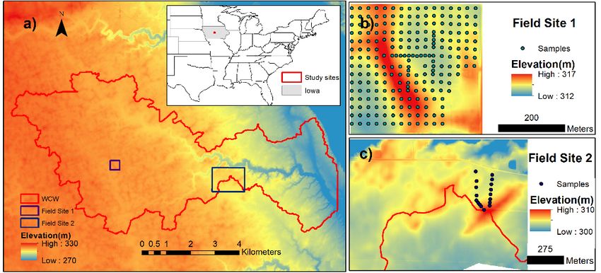
To test the hypotheses, we collected soil samples from two agricultural field sites in WCW
(Figure 2). ToOne
test (field
the hypotheses,
site 1) is anwe collected soil
intensively samples
sampled sitefrom
in thetwo agricultural
middle west offield sites in(Figure
the WCW WCW 2b).
(Figure 2). One (field site 1) is an intensively sampled site in the middle west of the WCW (Figure 2b).
A 25 × 25 m grid was created, and 230 soil samples were collected at grid nodes for SOC density and
A 25 × 25 m grid was created, and 230 soil samples were collected at grid nodes for SOC density and
SR rate estimation. Another site (field site 2) is about 4 km east from the field site 1 (Figure 2c). The
SR rate estimation. Another site (field site 2) is about 4 km east from the field site 1 (Figure 2c). The site
site includes two 300 m transects with observational SOC density and SR rate. At each location, three
includes two 300 m transects with observational SOC density and SR rate. At each location, three
samples were
samples collected
were collectedfrom
from0 0toto30
30cm
cmsoil
soil layer withinaa1 1××11mmquadrat
layer within quadrat using
using a push
a push probeprobe (3.2 cm
(3.2 cm
diameter).
diameter). The fields contain both Typic and Aquic soils. Nicollet soils are poorly drained and are are
The fields contain both Typic and Aquic soils. Nicollet soils are poorly drained and
located in lower
located in lower areas
areasand
and depressions,
depressions, and and Clarion
Clarion soilssoils are drained
are well well drained and in
and located located
hilltopsin[107].
hilltops
[107].Detailed
Detailed data
data collection
collection andand laboratory
laboratory analysis
analysis can becan be found
found in Li etin
al.Li et al.and
[7,25] [7,25] andetRitchie
Ritchie al. [22].et al.
[22].AAsummary
summary of of
thethe
used datadata
used is shown in Table
is shown 2. Generally,
in Table both sites
2. Generally, hadsites
both negative mean SR rates,
had negative mean SR
suggesting that soils were exported from these two sites within the period of 1960
rates, suggesting that soils were exported from these two sites within the period of 1960 to early 2000. to early 2000.
Figure 2. Locations
Figure 2. Locationsof study
of studyfields:
fields:(a)(a)Walnut
Walnut Creek Watershed(WCW),
Creek Watershed (WCW),(b)(b)
thethe intensive
intensive sampled
sampled
fieldfield
site site
1, and (c) (c)
1, and thethe
transect
transectfield
fieldsite
site2.
2.
Table 2. Mean and standard deviation (SD) of soil organic carbon (SOC) density and soil
redistribution rate (SR) at two field sites.
SOC (kg m−2) SR (Mg ha−1 year−1)
Mean SD Mean SD
Field Site 1 9.01 3.05 −5.9 21.6
Field Site 2 7.92 3.20 −4.35 30.8Soil Syst. 2020, 4, 32 9 of 19
Table 2. Mean and standard deviation (SD) of soil organic carbon (SOC) density and soil redistribution
rate (SR) at two field sites.
SOC (kg m−2 ) SR (Mg ha−1 year−1 )
Mean SD Mean SD
Field Site 1 9.01 3.05 −5.9 21.6
Field Site 2 7.92 3.20 −4.35 30.8
4.1.2. Terrain Analysis
Light detection and ranging (LiDAR)-derived DEMs were used to generate topographic metrics
of the two sites. The LiDAR data were acquired during the period 2007 to 2010 and are available via
the Iowa Geodata website. By use of inverse distance weighted interpolation, raw LiDAR data were
converted to DEMs with 3 m spatial resolution.
Fourteen metrics that were listed in Section 2 were generated on the basis of the 3 m DEM.
The metrics include altitude (A), slope gradient (G), profile curvature (P_Cur), plan curvature (Pl_Cur),
catchment area (CA), upslope slope (UpSl), downslope index (DI), flow path length (FPL), flow
accumulation (FA), topographic relief component 1 (TRPC1), topographic relief component 2 (TRPC2),
positive topographic openness (PTO), topographic wetness index (TWI), and stream power index
(SPI). The length—slope factor introduced in Section 2 was excluded due to its high correlation with
slope (r = 0.97) [7]. We used modules in SAGA to derive slope, P_Cur, Pl_Cur, CA, FA, PTO, DI, FPL,
TWI, SPI, and UpSl [6]. Topographic relief was generated on the basis of a maximum elevation map
within a specific area and a filtered 3 m DEM [40]. To reduce possible errors caused by an arbitrary
selection of a radius for a maximum elevation map, a series of radiuses were selected including 7.5
(relief7.5m ), 15 (relief15m ), 30 (relief30m ), 45 (relief45m ), 60 (relief60m ), 75 (relief75m ), and 90 m (relief90m ).
Principal component analysis (PCA) was applied to convert the relief maps into two independent relief
components (TRPC1 and TRPC2).
4.1.3. Statistical Analysis and Model Calibration
We used Spearman’s rank analysis to analyze topographic impacts on spatial patterns of SOC
density and SR rate. Then, we tested performances of OKr, TPCR, and TPCR-Kr models in predicting
the above two variables. OKr predicts unsampled locations by weighted averaging of nearby sampled
data, and the weights were derived on the basis of semivariogram analysis of the sampled data.
For the TPCR models, we first used PCR to analyze topographic metrics of all croplands within the
watershed. Components with loadings that explained more than 90% of the variance of all metrics
were used to construct topographic principal components (TPCs) used for TPCR models. TPCR-Kr
models combine the regression of the dependent variables with the kriging of the regression residuals.
Therefore, two steps were included for the TPCR-Kr model implementation: (1) analyzing residuals of
TPCR using semivariogram and OKr, and (2) summing the regression prediction and kriging prediction
of the residual.
Specifically, OKr and stepwise TPCR models were developed on the basis of SOC and SR
observations at the field site 1. The SOC density was log-transformed to meet the residual normality
assumption in linear regression. We used the Akaike information criterion (AIC) to select dependent
variables in stepwise models. We evaluated the model performances by comparing predictions with
observations in the transects. Residuals of the predictions over the transects were calculated and used
for developing TPCR-Kr models over field site 2.
Model efficiency was assessed on the basis of three criteria: the coefficient of determination (R2 ),
Nash—Sutcliffe efficiency (NSE), and the ratio of the root mean square error to the standard deviation
of measured data (RSR). Generally, the higher the R2 and NSE and the lower the RSR values are, the
better the model performs. If the NSE value is larger than 0.5 and the RSR is less than 0.7, the model is
considered as satisfactory.Soil Syst. 2020, 4, 32 10 of 19
4.2. Results and Discussion
4.2.1. Topographic Impacts on SOC and Soil Redistribution
Our results suggested that landscape topography significantly impacted soil properties and soil
processes even in relatively flat terrain. TWI was the most influential topographic metric and positively
impacted SOC density (Table 3). It also showed a high positive correlation with SR rates (Table 3).
Soil water conditions that TWI reflects can be a reason for these high correlations [40]. Generally, areas
with low TWI values tend to be drier than areas with high values. Therefore, the aerobic environments
in low water content areas would support rapid aerobic decomposition of soil C, leading to low SOC
storage [7,9,108,109]. Meanwhile, a location with high TWI usually suggests that the site has a large
catchment area and low slope gradient, which would promote sedimentation of fine particles with high
proportions of SOC content [110,111]. This further explained the high positive correlations between
TWI and SOC density, as well as TWI and SR rates in this study.
Table 3. Topographic impacts on soil organic carbon (SOC) and soil redistribution (SR) rate.
A G P_Cur Pl_Cur CA UpSl DI FPL FA TRPC1 TRPC2 PTO TWI SPI
−0.441 −0.669 −0.212 −0.336 0.537 −0.289 0.432 0.419 −0.225 0.665 −0.150 −0.583 0.722
SOC -
*** *** *** *** *** *** *** *** *** *** * *** ***
−0.441 −0.591 −0.225 −0.248 0.513 −0.170 0.404 0.437 −0.196 0.633 −0.488 0.605
SR - 0.128 *
*** *** *** *** *** ** *** *** ** *** *** ***
Note: *** p < 0.0001, ** p < 0.005, * p < 0.05. A is altitude; G is slope gradient; P_Cur and Pl_Cur are profile curvature
and plan curvature, respectively; CA is catchment area; UpSl is upslope slope; DI is downslope index; FPL is flow
path length; FA is flow accumulation; TRPC1 and TRPC2 are topographic relief principal components 1 and 2,
respectively; PTO is positive topographic openness; TWI is topographic wetness index; and SPI is stream power
index. The value in bold is correlation coefficient >0.5, and the value in red and bold indicates the highest correlation
coefficient for each soil property.
Topographic relief (TR) presented the highest positive correlation with SR rate and a high positive
correlation with SOC density. TRPC1 was mainly related to the large-scale relief maps (relief30m ,
relief45m , relief60m ), which exhibited landscape fluctuation over a large area, whereas TRPC2 was
dominated by the small-scale relief maps (relief7.5m ), showing location variation at a small location.
The substantial impacts of TRPC1 on SR rates and SOC density may have been due to its influences
on flow velocity. Areas with high TRPC1 values have large elevation differences from the most top
points, which accelerate flow velocity, causing more transport of soil from low relief (small elevation
difference) to the high relief (large elevation difference) areas [112,113]. Therefore, SR rates and SOC
density values were high in high TR locations.
Several other topographic metrics, such as G and CA, were also highly related to SOC density
and SR rate (r > 0.5). G and CA were related to flow velocity and flow accumulation, respectively.
This finding is similar to the study of Fox and Papanicolaou [114], which found that overland flow
regulated the incoming water and soil from uplands in a low-relief agricultural watershed.
4.2.2. Topography-Based Model Evaluations
Both TPCR and OKr models obtained satisfactory results in predicting SOC density and SR rate at
the field site 1, with high NSE (>0.5) and low RSR (and SR rate (r > 0.5). G and CA were related to flow velocity and flow accumulation, respectively.
This finding is similar to the study of Fox and Papanicolaou [114], which found that overland flow
regulated the incoming water and soil from uplands in a low-relief agricultural watershed.
4.2.2. Topography-Based Model Evaluations
Soil Syst. 2020, 4, 32 11 of 19
Both TPCR and OKr models obtained satisfactory results in predicting SOC density and SR rate
at the field site 1, with high NSE (>0.5) and low RSR (Soil Syst. 2020, 4, 32 12 of 19
transects. One possible reason for the deviations that existed after extrapolation may be related to field
management.
Soil Syst. 2020, 4, xEach production
FOR PEER REVIEW field has unique management history that can affect storage of
12 SOC
of 19
and movement
Soil Syst. of sediments
2020, 4, x FOR over the landscape [117,118].
PEER REVIEW 12 of 19
Figure 5. Comparison of topographic principal component regression (TPCR, blue data points) and
TPCR-kriging (TPCR-Kr, orange data points)-derived (a) soil organic carbon (SOC) density (kg m−2)
Figure 5.
Figure 5. Comparison
Comparison of of topographic
topographic principal
principal component
component regression
regression (TPCR,
(TPCR, blue
blue data
data points)
points) and
and
and (b) soil redistribution (SR) rate (Mg ha−1 year−1) predictions for observations at field site 2.
TPCR-kriging (TPCR-Kr, orangeorange data
data points)-derived
points)-derived (a)(a) soil
soil organic
organic carbon
carbon (SOC)
(SOC)density
density(kg
(kgm m−2
−2)
redistribution (SR)
and (b) soil redistribution (SR) rate
rate (Mg ha−1 year
(Mg ha −1
year−1) )predictions
−1
predictionsforforobservations
observationsatatfield
fieldsite
site2.2.
Figure 6. Maps
Figure Mapsof oflandscape
landscapecharacteristics
characteristicsand
andmodel-derived
model-derived soil property
soil maps
property at field
maps sitesite
at field 2: (a)
2:
bare
(a) soilsoil
bare image; (b) (b)
image; topographic principal
topographic component
principal component regression
regression(TPCR)-derived SOC
(TPCR)-derived SOCdensity; (c)
density;
Figure 6. Maps of landscape characteristics and model-derived soil property maps at field site 2: (a)
TPCR-kriging
(c) TPCR-kriging (TPCR-Kr)-derived
(TPCR-Kr)-derived SOC
SOC density; (d)
density; (d)elevation;
elevation;(e) TPCR-derived
TPCR-derived soil
(e)(TPCR)-derived redistribution
bare soil image; (b) topographic principal component regression SOC density; (c)
(SR) rate;
(SR) rate; and
and (f)
(f) TPCR-Kr-derived
TPCR-Kr-derived SRSR rate.
rate.
TPCR-kriging (TPCR-Kr)-derived SOC density; (d) elevation; (e) TPCR-derived soil redistribution
(SR) rate; and (f) TPCR-Kr-derived SR rate.
TPCR-Kr models reduced the estimation variances and were better fitted for the soil property
and TPCR-Kr
process predictions in transects,
models reduced which substantiated
the estimation variances and our
werethird hypothesis.
better Specifically,
fitted for the the
soil property
TPCR-Kr SOC model provided the same range as observations with a slope close to 1. The NSE
and process predictions in transects, which substantiated our third hypothesis. Specifically, the values
increasedSOC
TPCR-Kr frommodel
0.528 provided
to 0.761 with use of
the same TPCR
range and TPCR-Krwith
as observations SOC models,
a slope respectively,
close to 1. The NSEand RSR
valuesSoil Syst. 2020, 4, 32 13 of 19
TPCR-Kr models reduced the estimation variances and were better fitted for the soil property and
process predictions in transects, which substantiated our third hypothesis. Specifically, the TPCR-Kr
SOC model provided the same range as observations with a slope close to 1. The NSE values increased
from 0.528 to 0.761 with use of TPCR and TPCR-Kr SOC models, respectively, and RSR values decreased
from 0.687 to 0.489 with use of TPCR and TPCR-Kr SOC models, respectively. Use of the TPCR-Kr SR
also improved the accuracy relative to the TPCR SR model, as presented by the increased NSR and
decreased RSR values.
The improvement of the TPCR-Kr models suggested a possible use of local calibrations for
correcting regional TPCR models. A cropland field within a region has a unique management history,
which can increase deviations in measured soil properties from a soil map generated by a regional
TPCR model [117,118]. The spatial patterns of the soil properties under topographic influences as
produced by TPCR may be less variable than the estimated ranges for the observed parameters. As a
result, TPCR can produce accurate patterns of soil property distribution but the means and ranges of
the properties may be inaccurate. A relatively small number of samples could be collected from the
field of interest to adjust the topographic model using TPCR-Kr to better reflect the range in measured
values of the soil parameter. With this approach, map accuracy would improve.
In summary, the advantage of topographic models is the ease at which necessary data can be
acquired over large geographic areas by means of LiDAR mapping. Visual inspection of the bare soil
image and the regional TPCR map for SOC demonstrated remarkable high fidelity for a regional model
predicting spatial patterns of SOC on a distant cropland field with fine-scale detail. Application of
TPCR-Kr with inclusion of a relatively small number of local samples can localize the calibration for an
area of interest while retaining the high-fidelity spatial patterns.
Principal component analysis (PCA) of the geographic region can be performed independent of
physical sampling for soil characteristics. Sampling strategies can then be developed such that the full
range of principal components (PCs) are covered within the sample set. PCA also affords the ability to
test that a location is within the domain of the topographic model by use of repeated subsampling
of a landscape to generate a population of PC sets for statistical testing of differences from PCs of
the modeling domain. Li et al. [6] demonstrated that when topographic models are extrapolated to
a watershed scale, the TPCR models are superior to ordinary least square regression models, likely
because of reduced overfitting during calibration. The PCs used in the TPCR models were developed
at the watershed scale, providing better assurance that model parameters reflected the topography of
the larger setting.
5. Conclusions
This report reviewed the effects of landscape topography on soil properties and processes and
introduced five main groups of topography-based models. We then highlighted three models—OKr,
TPCR, and TPCR-Kr—by comparing the performances in SOC density and SR rate interpolations
and extrapolations in a case study. OKr provides analyses of spatial relations and TPCR considers
topographic information. Although the OKr models provided the best fits for SOC and SR calibrations,
the high accuracies require a large set of field sample data, which is often not available for many regions.
In contrast, the TPCR models utilized data only from remotely sensed data, providing cost-effective
methods to investigate soil spatial patterns. However, variations in climate, environment, and human
management may influence soil properties and processes, increasing estimation variances when
applying the regional TPCR model to different fields of interest [119–121]. TPCR-Kr improved the
model accuracy by including sample correction. The application of TPCR-Kr allowed local calibration
of the TPCR model to better reflect the mean and range of measured soil parameters. With a very
limited number of new samples, a regional topographic model can be adjusted to the local condition,
and spatial patterns of soil properties can be mapped with high fidelity.Soil Syst. 2020, 4, 32 14 of 19
Author Contributions: Conceptualization, X.L. and G.W.M.; methodology, X.L. and L.D.; writing—original draft
preparation, X.L.; writing—review and editing, G.W.M., S.L., and L.D; supervision, G.W.M.; project administration,
G.W.M.; funding acquisition, G.W.M. All authors have read and agreed to the published version of the manuscript.
Funding: This research was funded by the United State Department of Agriculture Natural Resources Conservation
Service in association with the Wetland Component of the National Conservation Effects Assessment Project
(NRCS 67-3A75-13-177).
Acknowledgments: This research was supported by the United State Department of Agriculture Natural Resources
Conservation Service in association with the Wetland Component of the National Conservation Effects Assessment
Project (NRCS 67-3A75-13-177).
Conflicts of Interest: The authors declare no conflict of interest.
References
1. Florinsky, I.V. Digital Terrain Analysis in Soil Science and Geology, 2nd ed.; Academic Press: Amsterdam,
The Netherlands, 2016.
2. Florinsky, I.V.; McMahon, S.; Burton, D.L. Topographic control of soil microbial activity: A case study of
denitrifiers. Geoderma 2004, 119, 33–53. [CrossRef]
3. Walker, P.H.; Hall, G.F.; Protz, R. Relation between landform parameters and soil properties. Soil Sci. Soc.
Am. J. 1968, 32, 101–104. [CrossRef]
4. Aandahl, A.R. The characterization of slope positions and their influence on the total nitrogen content of a
few virgin soils of western Iowa. Soil Sci. Soc. Am. J. 1949, 13, 449–454. [CrossRef]
5. Skidmore, A.K. A comparison of techniques for calculating gradient and aspect from a gridded digital
elevation model. Int. J. Geogr. Inf. Syst. 1989, 3, 323–334. [CrossRef]
6. Li, X.; McCarty, G.W. Use of principal components for scaling up topographic models to map soil redistribution
and soil organic carbon. J. Vis. Exp. 2018, e58189. [CrossRef] [PubMed]
7. Li, X.; McCarty, G.W.; Karlen, D.L.; Cambardella, C.A. Topographic metric predictions of soil redistribution
and organic carbon in Iowa cropland fields. Catena 2018, 160, 222–232. [CrossRef]
8. Li, X.; McCarty, G.W.; Lang, M.; Ducey, T.; Hunt, P.; Miller, J. Topographic and physicochemical controls on
soil denitrification in prior converted croplands located on the Delmarva Peninsula, USA. Geoderma 2018,
309, 41–49. [CrossRef]
9. Li, X.; McCarty, G.W.; Karlen, D.L.; Cambardella, C.A.; Effland, W. Soil organic carbon and isotope
composition response to topography and erosion in Iowa. J. Geophys. Res. Biogeosci. 2018, 123, 3649–3667.
[CrossRef]
10. Florinsky, I.V.; Eilers, R.G.; Manning, G.R.; Fuller, L.G. Prediction of soil properties by digital terrain
modelling. Environ. Model. Softw. 2002, 17, 295–311. [CrossRef]
11. Moore, I.D.; Gessler, P.E.; Nielsen, G.A.; Peterson, G.A. Soil attribute prediction using terrain analysis. Soil
Sci. Soc. Am. J. 1993, 57, 443–452. [CrossRef]
12. McBratney, A.B.; Odeh, I.O.A.; Bishop, T.F.A.; Dunbar, M.S.; Shatar, T.M. An overview of pedometric
techniques for use in soil survey. Geoderma 2000, 97, 293–327. [CrossRef]
13. Odeh, I.O.A.; McBratney, A.B.; Chittleborough, D.J. Spatial prediction of soil properties from landform
attributes derived from a digital elevation model. Geoderma 1994, 63, 197–214. [CrossRef]
14. Odeh, I.O.A.; McBratney, A.B.; Chittleborough, D.J. Further results on prediction of soil properties from
terrain attributes: Heterotopic cokriging and regression-kriging. Geoderma 1995, 67, 215–226. [CrossRef]
15. Bishop, T.F.A.; Mcbratney, A.B. A comparison of prediction methods for the creation of field-extent soil
property maps. Geoderma 2001, 103, 149–160. [CrossRef]
16. Moore, I.D.; Grayson, R.B.; Ladson, D.A.R. Digital terrain modelling: A review of hydrological,
geomorphological, and biological applications. Hydrol. Process. 1991, 5, 3–30. [CrossRef]
17. Janeau, J.L.; Bricquet, J.P.; Planchon, O.; Valentin, C. Soil crusting and infiltration on steep slopes in northern
Thailand. Eur. J. Soil Sci. 2003, 54, 543–553. [CrossRef]
18. Jun, H.; Wu, P.U.; Zhao, X. Effects of rainfall intensity, underlying surface and slope gradient on soil
infiltration under simulated rainfall experiments. Catena 2013, 104, 93–102.
19. Carter, B.J.; Ciolkosz, E.J. Slope gradient and aspect effects on soils developed from sandstone in Pennsylvania.
Geoderma 1991, 49, 199–213. [CrossRef]Soil Syst. 2020, 4, 32 15 of 19
20. Kenter, J. Carbonate platform flanks: Slope angle and sediment fabric. Sedimentology 1990, 37, 777–794.
[CrossRef]
21. Troch, P.; Van Loon, E.; Hilberts, A. Analytical solutions to a hillslope-storage kinematic wave equation for
subsurface flow. Adv. Water Resour. 2002, 25, 637–649. [CrossRef]
22. Ritchie, J.C.; McCarty, G.W.; Venteris, E.R.; Kaspar, T.C. Soil and soil organic carbon redistribution on the
landscape. Geomorphology 2007, 89, 163–171. [CrossRef]
23. Li, Q.Y.; Fang, H.Y.; Sun, L.Y.; Cai, Q.G. Using the 137 Cs technique to study the effect of soil redistribution on
soil organic carbon and total nitrogen stocks in an agricultural catchment of Northeast China. Land Degrad.
Dev. 2014, 25, 350–359. [CrossRef]
24. Gessler, P.E.; Moore, I.D.; McKenzie, N.J.; Ryan, P.J. Soil-landscape modelling and spatial prediction of soil
attributes. Int. J. Geogr. Inf. Syst. 1995, 9, 421–432. [CrossRef]
25. Li, X.; McCarty, G.W. Application of topographic analyses for mapping spatial patterns of soil properties.
In Earth Observation and Geospatial Analyses geometry; Pepe, A., Ed.; IntechOpen: London, UK, 2019; pp. 1–32.
[CrossRef]
26. Dai, W.; Huang, Y. Relation of soil organic matter concentration to climate and altitude in zonal soils of
China. Catena 2006, 65, 87–94. [CrossRef]
27. Wilson, J.P.; Gallant, J.C. Digital terrain analysis. In Terrain Analysis: Principles and Applications; Wilson, J.P.,
Gallant, J.C., Eds.; John Wiley & Sons Ltd.: New York, NY, USA, 2000; pp. 1–27.
28. Hjerdt, K.N. A new topographic index to quantify downslope controls on local drainage. Water Resour. Res.
2004, 40, 1–6. [CrossRef]
29. Seibert, J.; Stendahl, J.; Sørensen, R. Topographical influences on soil properties in boreal forests. Geoderma
2007, 141, 139–148. [CrossRef]
30. Summerfield, M.A.; Hulton, N.J. Natural controls of fluvial denudation rates in major world drainage basins.
J. Geophys. Res. 1994, 99, 13871–13883. [CrossRef]
31. Kasai, M.; Marutani, T.; Reid, L.M.; Trustrum, N.A. Estimation of temporally averaged sediment delivery
ratio using aggradational terraces in headwater catchments of the Waipaoa River, North Island, New Zealand.
Earth Surf. Process. Landf. 2001, 26, 1–16. [CrossRef]
32. Yanosek, K.A.; Foltz, R.B.; Dooley, J.H. Performance assessment of wood strand erosion control materials
among varying slopes, soil textures, and cover amounts. J. Soil Water Conserv. 2006, 61, 45–51.
33. Schubert, J. Hydraulic aspects of riverbank filtration—Field studies. J. Hydrol. 2002, 266, 145–161. [CrossRef]
34. Doody, D.; Moles, R.; Tunney, H.; Kurz, I.; Bourke, D.; Daly, K.; O’Regan, B. Impact of flow path length and
flow rate on phosphorus loss in simulated overland flow from a humic gleysol grassland soil. Sci. Total
Environ. 2006, 372, 247–255. [CrossRef] [PubMed]
35. Mitasova, H.; Hofierka, J.; Zlocha, M.; Iverson, L.R. Modeling topographic potential for erosion and deposition
using GIS. Int. J. Geogr. Inf. Syst. 1996, 10, 629–641. [CrossRef]
36. Zhang, H.; Yang, Q.; Li, R.; Liu, Q.; Moore, D.; He, P.; Ritsema, C.J.; Geissen, V. Extension of a GIS procedure
for calculating the RUSLE equation LS factor. Comput. Geosci. 2013, 52, 177–188. [CrossRef]
37. Gessler, P.E.; Chadwick, O.A.; Chamran, F.; Althouse, L.; Holmes, K. Modeling soil–landscape and ecosystem
properties using terrain attributes. Soil Sci. Soc. Am. J. 2000, 64, 2046–2056. [CrossRef]
38. Dahal, R.K.; Hasegawa, S.; Nonomura, A.; Yamanaka, M.; Masuda, T.; Nishino, K. GIS-based
weights-of-evidence modelling of rainfall-induced landslides in small catchments for landslide susceptibility
mapping. Environ. Geol. 2008, 54, 311–324. [CrossRef]
39. Yokoyama, R.; Shlrasawa, M.; Pike, R.J. Visualizing topography by openness: A new application of image
processing to digital elevation models. Photogramm. Eng. Remote Sens. 2002, 68, 257–265.
40. Lang, M.W.; McCarty, G.W.; Oesterling, R.; Yeo, I.Y. Topographic metrics for improved mapping of forested
wetlands. Wetlands 2013, 33, 141–155. [CrossRef]
41. Pei, T.; Qin, C.Z.; Zhu, A.X.; Yang, L.; Luo, M.; Li, B.; Zhou, C. Mapping soil organic matter using the
topographic wetness index: A comparative study based on different flow-direction algorithms and kriging
methods. Ecol. Indic. 2010, 10, 610–619. [CrossRef]
42. Lang, M.W.; McCarty, G.W. Lidar intensity for improved detection of inundation below the forest canopy.
Wetlands 2009, 29, 1166–1178. [CrossRef]
43. Tagil, S.; Jenness, J. GIS-based automated landform classification and topographic, landcover and geologic
attributes of landforms around the Yazoren Polje, Turkey. J. Appl. Sci. 2008, 8, 910–921. [CrossRef]Soil Syst. 2020, 4, 32 16 of 19
44. Conforti, M.; Aucelli, P.P.C.; Robustelli, G.; Scarciglia, F. Geomorphology and GIS analysis for mapping gully
erosion susceptibility in the Turbolo stream catchment (Northern Calabria, Italy). Nat. Hazards 2011, 56,
881–898. [CrossRef]
45. Moore, I.; Nieber, J. Landscape assessment of soil erosion and nonpoint source pollution. J. Minn. Acad. Sci.
1989, 55, 18–25.
46. Desmet, P.J.J.; Govers, G. A GIS procedure for automatically calculating the USLE LS factor on topographically
complex landscape units. J. Soil Water Conserv. 1996, 51, 427–433.
47. Wischmeier, W.H.; Smith, D.D. Predicting Rainfall Erosion Losses—A Guide to Conservation Planning; U.S.
Department of Agriculture Handbook: Washington, DC, USA, 1978.
48. Babak, O.; Deutsch, C.V. Estimation in a Finite Domain: Fixing the String Effect; Centre for Computational
Geostatistics; Department of Civil & Environmental EngineeringUniversity of Alberta: Alberta, BC, Canada,
2006; pp. 1–19.
49. Ersahin, S. Comparing ordinary kriging and cokriging to estimate infiltration rate. Soil Sci. Soc. Am. J. 2003,
67, 1848–1855. [CrossRef]
50. Burgess, T.M.; Webster, R. Optimal interpolation and isarithmic mapping of soil properties: I The
semi-variogram and punctual kriging. J. Soil Sci. 1980, 31, 315–331. [CrossRef]
51. Eldeiry, A.A.; Garcia, L.A. Comparison of ordinary kriging, regression kriging, and cokriging techniques to
estimate soil salinity using LANDSAT images. J. Irrig. Drain. Eng. 2010, 136, 355–364. [CrossRef]
52. Zhu, Q.; Lin, H.S. Comparing ordinary kriging and regression kriging for soil properties in contrasting
landscapes. Pedosphere 2010, 20, 594–606. [CrossRef]
53. Yao, X.; Fu, B.; Lü, Y.; Sun, F.; Wang, S.; Liu, M. Comparison of four spatial interpolation methods for
estimating soil moisture in a complex terrain catchment. PLoS ONE 2013, 8, e54660. [CrossRef]
54. Bilgili, A.V. Spatial assessment of soil salinity in the Harran Plain using multiple kriging techniques.
Environ. Monit. Assess. 2013, 185, 777–795. [CrossRef]
55. Sumfleth, K.; Duttmann, R. Prediction of soil property distribution in paddy soil landscapes using terrain
data and satellite information as indicators. Ecol. Indic. 2008, 8, 485–501. [CrossRef]
56. Li, Q.Q.; Yue, T.X.; Wang, C.Q.; Zhang, W.J.; Yu, Y.; Li, B.; Yang, J.; Bai, G.C. Spatially distributed modeling of
soil organic matter across China: An application of artificial neural network approach. Catena 2013, 104,
210–218. [CrossRef]
57. Herbst, M.; Diekkrüger, B.; Vereecken, H. Geostatistical co-regionalization of soil hydraulic properties in a
micro-scale catchment using terrain attributes. Geoderma 2006, 132, 206–221. [CrossRef]
58. Motaghian, H.R.; Mohammadi, J. Spatial estimation of saturated hydraulic conductivity from terrain
attributes using regression, kriging, and artificial neural networks. Pedosphere 2011, 21, 170–177. [CrossRef]
59. Bourennane, H.; King, D.; Couturier, A. Comparison of kriging with external drift and simple linear regression
for predicting soil horizon thickness with different sample densities. Geoderma 2000, 97, 255–271. [CrossRef]
60. Zadeh, I.A. Fuzzy sets. Inf. Control 1965, 8, 338–353. [CrossRef]
61. Brulé, J.F. Fuzzy Systems-a Tutorial. Pacific Northwest National. 1985. Available online: http://www.
jimbrule.com/fuzzytutorial.html (accessed on 1 January 2011).
62. McBratney, A.B.; Odeh, I.O.A. Application of fuzzy sets in soil science: Fuzzy logic, fuzzy measurements
and fuzzy decisions. Geoderma 1997, 77, 85–113. [CrossRef]
63. Lark, R.M. Soil-landform relationships at within-field scales: An investigation using continuous classification.
Geoderma 1999, 92, 141–165. [CrossRef]
64. Zhu, A.X.; Hudson, B.; Burt, J.; Lubich, K.; Simonson, D. Soil mapping using GIS, expert knowledge, and
fuzzy logic. Soil Sci. Soc. Am. J. 2001, 65, 1463–1472. [CrossRef]
65. Zhu, A.X.; Band, L.E.; Dutton, B.; Nimlos, T.J. Automated soil inference under fuzzy logic. Ecol. Model. 1996,
90, 123–145. [CrossRef]
66. Odeh, I.O.A.; Chittleborough, D.J.; McBratney, A.B. Soil pattern recognition with fuzzy-c-means: Application
to classification and soil-landform interrelationships. Soil Sci. Soc. Am. J. 1992, 56, 505–516. [CrossRef]
67. McBratney, A.B.; De Gruijter, J.J. A continuum approach to soil classification by modified fuzzy k-means
with extragrades. J. Soil Sci. 1992, 43, 159–175. [CrossRef]
68. Qi, F.; Zhu, A.X.; Harrower, M.; Burt, J.E. Fuzzy soil mapping based on prototype category theory. Geoderma
2006, 136, 774–787. [CrossRef]You can also read