The effects of surface fossil magnetic fields on massive star evolution - III. The case of τ Sco
←
→
Page content transcription
If your browser does not render page correctly, please read the page content below
MNRAS 504, 2474–2492 (2021)                                                                                                         doi:10.1093/mnras/stab893
Advance Access publication 2021 March 27

The effects of surface fossil magnetic fields on massive star evolution – III.
The case of τ Sco
Z. Keszthelyi ,1‹ G. Meynet,2 F. Martins,3 A. de Koter1,4 and A. David-Uraz                                              5,6,7
1 Anton  Pannekoek Institute for Astronomy, University of Amsterdam, Science Park 904, 1098 XH Amsterdam, the Netherlands
2 Geneva   Observatory, University of Geneva, Maillettes 51, 1290 Sauverny, Switzerland
3 LUPM, Université de Montpellier, CNRS, Place Eugène Bataillon, F-34095 Montpellier, France
4 Institute of Astronomy, KU Leuven, Celestijnenlaan 200D, 3001 Leuven, Belgium
5 Department of Physics and Astronomy, University of Delaware, Newark, DE 19716, USA
6 Department of Physics and Astronomy, Howard University, Washington, DC 20059, USA
7 Center for Research and Exploration in Space Science and Technology, and X-ray Astrophysics Laboratory, NASA/GSFC, Greenbelt, MD 20771, USA

                                                                                                                                                                   Downloaded from https://academic.oup.com/mnras/article/504/2/2474/6195517 by guest on 24 October 2021
Accepted 2021 March 19. Received 2021 March 17; in original form 2020 October 26

ABSTRACT
τ Sco, a well-studied magnetic B-type star in the Upper Sco association, has a number of surprising characteristics. It rotates
very slowly and shows nitrogen excess. Its surface magnetic field is much more complex than a purely dipolar configuration
which is unusual for a magnetic massive star. We employ the CMFGEN radiative transfer code to determine the fundamental
parameters and surface CNO and helium abundances. Then, we employ MESA and GENEC stellar evolution models accounting
for the effects of surface magnetic fields. To reconcile τ Sco’s properties with single-star models, an increase is necessary in the
efficiency of rotational mixing by a factor of 3–10 and in the efficiency of magnetic braking by a factor of 10. The spin-down
could be explained by assuming a magnetic field decay scenario. However, the simultaneous chemical enrichment challenges
the single-star scenario. Previous works indeed suggested a stellar merger origin for τ Sco. However, the merger scenario also
faces similar challenges as our magnetic single-star models to explain τ Sco’s simultaneous slow rotation and nitrogen excess.
In conclusion, the single-star channel seems less likely and versatile to explain these discrepancies, while the merger scenario
and other potential binary-evolution channels still require further assessment as to whether they may self-consistently explain
the observables of τ Sco.
Key words: stars: abundances – stars: evolution – stars: individual: τ Sco – stars: magnetic field – stars: massive – stars: rotation.

                                                                                    et al. 2013; Shultz et al. 2018). Additional observations confirmed
1 I N T RO D U C T I O N
                                                                                    these findings, showing that the magnetic energy density indeed
τ Scorpii (HD 149438) is a magnetic massive B0.2 V star in the                      resides in higher order spherical harmonic components, which clearly
Upper Sco association, which has been well-studied for almost an                    implies that the field is complex (Donati & Landstreet 2009; Shultz
entire century (e.g. Struve & Dunham 1933; Unsöld 1942; Traving                    et al. 2019a,b). Based on the circular (Stokes V) spectropolarimetric
1955; Aller, Faulkner & Norton 1966; Lamers & Rogerson 1978;                        data set, Kochukhov & Wade (2016) produced possible magnetic
Wolff & Heasley 1985; Kilian 1992; Howk et al. 2000). In addition                   field maps of τ Sco. However, the specific geometry needs to be
to a large number of observations in the optical band, there is also                known to produce a unique magnetic field map. This relies on further
a wealth of multiwavelength observations, including X-ray (e.g.                     observations using linear polarimetry (Stokes Q, U) to constrain the
Macfarlane & Cassinelli 1989; Cohen, Cassinelli & Waldron 1997;                     magnetic field modulus.
de Messieres et al. 2001; Cohen et al. 2003; Mewe et al. 2003; Ignace                  Interestingly, despite the non-uniqueness problem, the magnetic
et al. 2010; Nazé et al. 2014; Fletcher et al. 2018), ultraviolet (e.g.            field maps produced from the spectropolarimetric observations are
Walborn & Panek 1984; Peters & Polidan 1985; Rogerson & Ewell                       quite reminiscent of the magnetohydrodynamic (MHD) simulations
1985; Cowley & Merritt 1987; Snow et al. 1994), and infrared (e.g.                  of Braithwaite (2008) who demonstrated that an initial seed field
Waters et al. 1993; Zaal et al. 1999; Repolust et al. 2005).                        can relax into a stable non-axisymmetric equilibrium. Indeed, the
   Spectropolarimetric observations of τ Sco by Donati et al. (2006)                decade-long spectropolarimetry suggests that the field is stable and
led to the discovery of a surface magnetic field, which is unusually                of fossil origin.
complex compared to other B-type stars whose field measurements                        Using the magnetic oblique rotator model (Stibbs 1950), the
can usually be reconciled with a dipolar configuration (e.g. Petit                  rotation period of the star is constrained to 41.033 ± 0.002 d (Donati
                                                                                    et al. 2006). Depending on the assumed stellar radius, this yields
                                                                                    a surface equatorial rotational velocity of ≈5 km s−1 . Considering
   E-mail: z.keszthelyi@uva.nl                                                     measurements of the projected rotational velocity (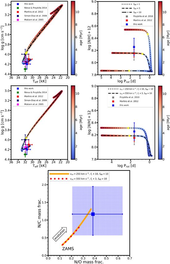
The effects of surface fossil magnetic fields on massive star evolution – III                               2475
Hardorp & Scholz 1970; Mokiem et al. 2005; Simón-Dı́az et al.              can firmly exclude the possibility that the star formed and evolved in
2006; Nieva & Przybilla 2014; Cazorla et al. 2017a, and see also            isolation, having acquired its fossil field during the assembly process.
Appendix B), it is clear that the present-day surface rotation of τ Sco     The purpose of this work therefore is, first, to re-assess stellar and
is very slow.                                                               surface properties, including its age and nitrogen abundance, and to
    Several authors, e.g. Kilian (1992), Morel, Hubrig & Briquet            comprehensively explore whether these empirical characteristics can
(2008), Przybilla et al. (2010), and Martins et al. (2012) measured         be reconciled with single-star evolutionary models that account for
the surface abundance of CNO elements. Their results are in                 surface magnetic field effects; and, second, to discuss implications
excellent agreement, strongly indicating nitrogen excess (log [N/H]         of these properties for merger models.
+ 12 = 8.15 ± 0.15, 8.15 ± 0.20, 8.16 ± 0.12, and 8.15 ± 0.06                  This paper is part of a series in which we aim to explore the effects
by number fraction, respectively). This means that τ Sco is highly          of surface fossil magnetic fields on massive star evolution. In the
enriched in core-processed material, by at least a factor of 3 compared     first paper of the series (Keszthelyi et al. 2019, hereafter Paper I), we
to the solar baseline. Helium abundance measurements are more               used the Geneva stellar evolution code (GENEC; Eggenberger et al.
uncertain. Previously obtained values (e.g. He/H = 0.085 by number          2008; Ekström et al. 2012; Georgy et al. 2013; Groh et al. 2019;
fraction from Wolff & Heasley 1985; He/H = 0.10 ± 0.025 from

                                                                                                                                                        Downloaded from https://academic.oup.com/mnras/article/504/2/2474/6195517 by guest on 24 October 2021
                                                                            Murphy et al. 2021) to explore the cumulative impact of magnetic
Kilian 1992; Y = 0.28 ± 0.03 by mass fraction from Przybilla                mass-loss quenching, magnetic braking, and field evolution. In
et al. 2010) are very close to the solar helium baseline (Grevesse,         the second paper (Keszthelyi et al. 2020, hereafter Paper II), we
Noels & Sauval 1996; Asplund, Grevesse & Sauval 2005; Asplund               implemented and studied massive star magnetic braking in the
et al. 2009), which would be compatible with expectations of a single       Modules for Experiments in Stellar Astrophysic (MESA) software
star in its early main sequence evolution. Although still overlapping       instrument (Paxton et al. 2011, 2013, 2015, 2018, 2019), detailing
within uncertainty, Mokiem et al. 2005 obtained He/H = 0.12+0.04    −0.02   the magnetic and rotational evolution, and confronting the models
by number fraction, which could point towards a slight excess in the        with a sample of observed magnetic B-type stars from Shultz et al.
surface helium abundance.                                                   (2018). A key finding of Paper II is that presently slowly rotating
    Nieva & Przybilla (2014) measured the stellar parameters of             magnetic stars may originate from either slow or fast rotators at the
τ Sco and based on its position on the Hertzsprung–Russell diagram          zero-age main sequence (ZAMS).
concluded that it is a blue straggler star that is much younger than the       The paper is organized as follows. In Section 2, we perform atmo-
association it belongs to, suggesting that it could possibly originate      spheric modelling, particularly focusing on the CNO elements and
from a stellar merger. Indeed, Ferrario et al. (2009) suggested that the    helium abundance. In Section 3, we carry out numerical experiments
origin of fossil magnetic fields may be stellar merger events. Further      with stellar evolution models. In Section 4, we discuss the impact
work by Schneider et al. (2016) explored this scenario and argued           of the initial assumptions and confront empirical evidence with our
that τ Sco could be rejuvenated via a merger process.                       results. Finally, we summarize our findings in Section 5.
    Recently Schneider et al. (2019) presented 3D MHD simulations
of stellar mergers and Schneider et al. (2020) implemented the results
                                                                            2 AT M O S P H E R I C M O D E L L I N G
into 1D stellar evolution models to follow the long-term evolution of
the post-merger object. These simulations showed that i) a seed field
                                                                            2.1 Determination of fundamental parameters
can be amplified to a strong magnetic field in the merger process and
ii) the post-merger object evolves seemingly as a single star, although     We have used the code CMFGEN (Hillier & Miller 1998) to determine
with an unusual internal chemical composition. Nonetheless, some            the fundamental stellar parameters of τ Sco. CMFGEN computes
important observables of τ Sco (such as the ≈ 5 km s−1 rotational           atmosphere models in non-LTE, spherical geometry, and includes
velocity and the factor of 3 nitrogen enrichment) are not yet               outflows and line-blanketing. A complete description of the code is
compatible with the current modelling efforts as they predict either        presented in Hillier & Miller (1998) and we refer the reader to this
modest rotation (50 km s−1 , which is still an order of magnitude larger    publication for further information.
than the observed value) with no nitrogen excess, or fast rotation             To the best of our knowledge, there is no atmosphere code for hot,
(400 km s−1 ) with nitrogen excess (see figs 3 and 5 of Schneider           massive stars (including non-LTE effects, sphericity, and winds),
et al. 2020). The only solution thus far that predicts sufficiently slow    which includes polarization in the radiative transfer equation. For
rotation (but no nitrogen excess) is a model with a constant surface        lower mass stars, Khan & Shulyak (2006) showed that the extra
magnetic dipole moment of μB = 1040 G cm3 corresponding to an               line-blanketing caused by Zeeman splitting had little impact on
approximately 270 kG field at the surface of a star with a radius of 5      the emergent spectrum, especially in the field strength regime of
R . Such a strong field is reached in the 3D MHD merger simulation         τ Sco. The expected Zeeman splitting of helium and CNO lines is
(Schneider et al. 2019), however, since the field strength remains          undetectable in individual lines unless the magnetic field is extremely
quasi-constant on the main sequence, it is far too strong compared to       strong (which is why field-detection techniques relying on many lines
any known OBA star and, in particular, to τ Sco’s measured surface          are used; Donati & Landstreet 2009), hence the use of non-polarized
field strength of a few hundred G (Donati et al. 2006; Shultz et al.        synthetic spectra is justified. Krtička (2018) showed that polarized
2018, and further details in Appendix B).                                   radiative transfer has little effect on radiative driving so that mass-
    These significant findings pose important questions, for example,       loss rates should not be affected. However, the presence of a magnetic
i) are all fossil magnetic fields generated via a stellar merger event,     field confines the expanding wind, leading to non-spherical effects
and ii) can we confidently identify signs of a past stellar merger event    that need to be taken into account when studying the details of stellar
and its evolutionary consequences when studying a star? This makes          winds in magnetic OB stars (e.g. ud-Doula 2017). In the present
τ Sco a valuable laboratory to further our understanding of magnetic        study, we focus on photospheric parameters which should not be
massive stars and for this reason the current discrepancies between         severely affected by the use of ‘non-magnetic’ models.
models and observations need to be studied in more detail.                     To determine the main fundamental parameters, we relied on
    The prospect of τ Sco being a merger product is intriguing. Of          a grid of CMFGEN models covering the effective temperatures
course, the validity of this scenario would be strengthened if one          and surface gravities of hot main sequence stars. We also used

                                                                                                                 MNRAS 504, 2474–2492 (2021)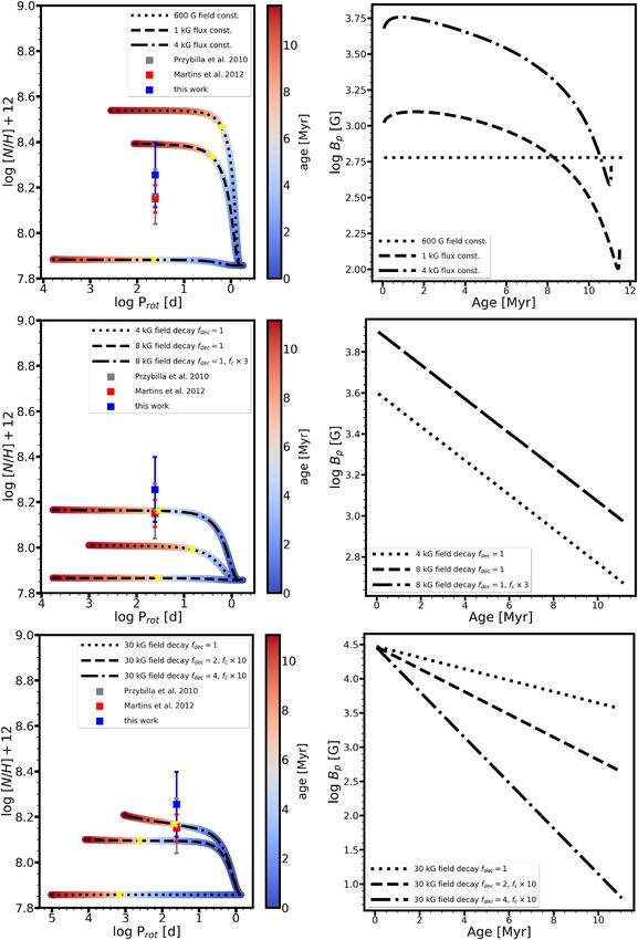
2476        Z. Keszthelyi et al.
the spectrum of τ Sco presented by Martins et al. (2012). It is                 We also investigated the possibility that τ Sco is enriched in
an average spectrum built from observations conducted with the               helium. To this extent, we ran models with He/H between 0.1 (the
spectropolarimeter ESPaDOnS at CFHT. It covers the wavelength                reference value) and 0.2. We used the following lines to estimate the
range 3800–6800 Å at a spectral resolution of about 65 000. In               goodness of fit:
this spectrum, we isolated the classical indicators to determine
                                                                               (i) Helium: He I 4026, He II 4200, He I 4388, He I 4471, He II 4542,
the effective temperature and surface gravity, namely He I 4471,
                                                                             He I 4713, He I 4921, He II 5412, He I 6680.
He II 4542, He II 5412, H γ and H β. We subsequently looked
for the best-fitting models using a χ 2 minimization process. We               The best fits were obtained for models with He/H = 0.11 ± 0.01.
found Teff = 31 500 ± 1000 K and log g = 4.2 ± 0.1 cm s−2 . For              This corresponds to Y = 0.30 ± 0.02 in mass fraction, implying a
consistency, the process was repeated with additional helium and             modest enrichment compared to the baseline value of Yini = 0.266.
Balmer lines and consistent results were obtained.                           The results are summarized in Table 1.
   In this process, we used a projected rotational velocity of 9 km s−1
and a macroturbulence of 10 km s−1 . The former was obtained from
                                                                             3 E VO L U T I O N A RY M O D E L L I N G

                                                                                                                                                              Downloaded from https://academic.oup.com/mnras/article/504/2/2474/6195517 by guest on 24 October 2021
the Fourier transform method (see Simón-Dı́az & Herrero 2007)
applied to O III 5592 and He I 4713. To determine the level of macro-        Evolutionary models were computed with two different codes,
turbulence, we convolved spectra from our grid and with parameters           Modules for Experiments in Stellar Astrophysics (MESA, Paxton
close to the final values with a rotational profile, an instrumental         et al. 2011, 2013, 2015, 2018, 2019) and the Geneva stellar evolution
one, and a radial-tangential profile mimicking macroturbulence. We           code (GENEC, Eggenberger et al. 2008; Ekström et al. 2012; Georgy
constrained the macroturbulence velocity by fitting He I 4713.               et al. 2013; Paper I). The two codes are sufficiently different that
   To constrain the luminosity of τ Sco, we computed the bolometric          they provide independent tests. In particular, the implementations
correction from Teff and the relation of Martins & Plez (2006). The          of angular momentum transport and loss are different (see Paper II,
extinction was estimated from the colour excess E(B − V) using the           Appendix A).
intrinsic (B − V)0 colour of Martins & Plez (2006). With the new
distance of d = 195 ± 42 pc from Gaia DR2, we finally obtained
log (L/L ) = 4.56 ± 0.20. Using the radius obtained from Teff and           3.1   MESA   modelling: setup
L/L , as well as the projected rotational velocity, and assuming an
                                                                             The general model parameters we adopt in MESA are as follows. A
inclination of about 90◦ , we find a rotation period of 36 d. This is in
                                                                             solar metallicity of Z = 0.014 is adopted with the Asplund et al.
excellent agreement with the 41 d found by Donati et al. (2006) from
                                                                             (2009) mixture of metals; isotopic ratios are from Lodders (2003).
spectropolarimetric measurements.
                                                                             The mixing efficiency in the convective core is treated by adopting
                                                                             α MLT = 2.0. Exponential overshooting is used above the convective
2.2 Surface abundances                                                       core with fov = 0.034 and f0 = 0.006 (Herwig 2000; Paxton et al.
                                                                             2013). This would approximately correspond to extending the
We determined the surface abundances of carbon, nitrogen, oxygen,
                                                                             convective core by 25 per cent of the local pressure scale height (thus
and helium. For each element, we computed atmosphere models and
                                                                             α ov = 0.25) in a non-rotating model.1 The OPAL opacity tables are
synthetic spectra with the set of fundamental parameters derived in
                                                                             used (Rogers & Iglesias 1992). The mass-loss scheme is adopted
Section 2.1 but different chemical compositions. We then used a set
                                                                             from de Jager, Nieuwenhuijzen & van der Hucht (1988).2 This mass-
of selected lines of each element to perform a χ 2 minimization and
                                                                             loss rate is then systematically scaled by the magnetic mass-loss
find the best-fitting model. These lines included in the analysis are:
                                                                             quenching parameter fB and rotational enhancement frot (see Paper II).
   (i) Carbon: C III 4056, C III 4068, C III 4070, C II 4075, C III 4665,       To account for rotationally induced instabilities which lead to
C III 4667, C II 5133, C II 5144, C II 5151, C II 5250, C III 5254,          chemical mixing, we use MESA’s default parametrization in a
C IV 5802, C IV 5812, C III 5827, C III 6205, C II 6578, C II 6583,          fully diffusive approach. The diffusion coefficients arising from
C III 6744.                                                                  dynamical and secular shear instabilities (Endal & Sofia 1978;
   (ii) Nitrogen: N II 3995, N II 4004, N II 4035, N III 4044, N III 4196,   Pinsonneault et al. 1989), Eddington-Sweet circulation (Eddington
N III 4216, N II 4447, N III 4511, N III 4515, N II 4602, N II 4607,         1925; Sweet 1950), Solberg-Høiland (Solberg 1936; Høiland 1941),
N III 4615, N II 4621, N III 4634, N III 4640, N II 4788, N II 4803,         and Goldreich-Schubert-Fricke instabilities (Goldreich & Schubert
N II 4995, N II 5001, N II 5005, N II 5011, N II 5026, N II 5045,            1967; Fricke 1968) are included. The Spruit–Tayler dynamo (Spruit
N II 5678, N II 5680.
   (iii) Oxygen: O II 3913, O II 3954, O II 3983, O II 4277, O II 4278,
                                                                                              ov = 0.1−0.5 is presently considered plausible based on
                                                                             1 A range of α
O II 4283, O II 4305, O II 4316, O II 4318, O II 4321, O II 4354,
O II 4367, O II 4370, O II 4397, O II 4415, O II 4417, O II 4453,            asteroseismic measurements as well as multidimensional hydrodynamic
                                                                             simulations (e.g. Herwig 2000; Meakin & Arnett 2007; Moravveji et al.
O II 4489, O II 4491, O II 4592, O II 4597, O II 4603, O II 4610,
                                                                             2015; Pápics et al. 2017; ). See recently Kaiser et al. (2020) and references
O II 4662, O II 4676, O II 4678, O II 4700, O II 4705, O III 5592.
                                                                             therein. We test other values in Appendix A, none the less, the precise choice
  We obtained the following values of surface abundances in                  of the overshooting parameter does not play an important role here as without
number fractions: C/H = 1.8+0.9          −4             +0.8    −4
                                −0.7 · 10 , N/H= 1.8−0.6 · 10 , and
                                                                             efficient envelope mixing, the surface composition will remain unaltered.
                                                                             2 This specific choice is made because the de Jager et al. (1988) mass-loss
          +2.0    −4
O/H= 4.1−1.3 · 10 . For these determinations, we used a microtur-
                                                                             rates in this mass and temperature range are slightly higher than the Vink,
bulent velocity of 2 km s−1 . A larger value would lead to excessive
                                                                             de Koter & Lamers (2001) rates, consequently they (very minimally) also
broadening, as, for instance, evidenced in the N II doublet at 5001 Å.       aid the spin-down of the star (e.g. Keszthelyi, Puls & Wade 2017). However,
The reduced microturbulence compared to the study of Martins et al.          we tested models with both mass-loss prescriptions and found that they lead
(2012) explains the slightly larger N/H (1.8 · 10−4 in the present study     to completely negligible differences in this study. This is expected since the
versus 1.4 · 10−4 by Martins et al. 2012). The best-fitting synthetic        mass-loss rates during the early evolution of the models are on the order of
spectrum is shown in Fig. 1.                                                 Ṁ ≈ 10−9 − 10−8 M yr−1 .

MNRAS 504, 2474–2492 (2021)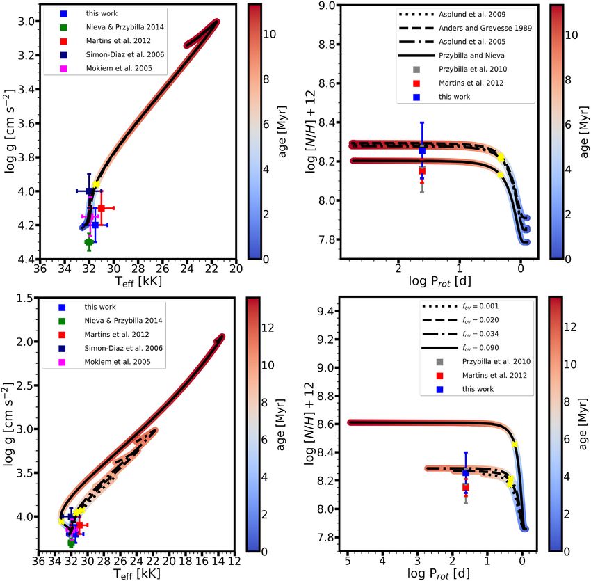
The effects of surface fossil magnetic fields on massive star evolution – III                                2477

                                                                                                                                                      Downloaded from https://academic.oup.com/mnras/article/504/2/2474/6195517 by guest on 24 October 2021
                                Figure 1. Best-fitting model (red) compared to the observed spectrum (black) of τ Sco.

Table 1. Stellar parameters and surface abundances in number fractions        2002; Tayler 1973) is not adopted. To consider the inhibiting impact
obtained from atmospheric modelling.                                          of composition gradients, ∇μ is scaled by fμ = 0.05 when calculating
                                                                              stability criteria for chemical mixing (Yoon, Langer & Norman 2006;
log (L/L )                                            4.56 ± 0.20            Brott et al. 2011; Paxton et al. 2013).
Teff (kK)                                               31.5 ± 1                 In MESA, angular momentum transport is modelled as a diffusive
log g (cm s−2 )                                         4.2 ± 0.1
                                                                              process. This means that angular momentum is only transported
 sin i (km s−1 )                                           9                 in one (outward) direction. The stellar core has a constant angular
mac (km s−1 )                                             10                 velocity profile. Close to the core-envelope boundary (at q = 0.4,
mic (km s−1 )                                              2                 i.e. at the layer encompassing 40 per cent of the total mass), we
C/H                                                   1.8+0.9
                                                         −0.7 · 10
                                                                   −4
                                                                              set the lower boundary to apply magnetic braking (see below).
N/H                                                   1.8+0.8
                                                         −0.6 · 10
                                                                   −4         Therefore, we assume that the magnetic field spreads through the
O/H                                                   4.1+2.0
                                                         −1.3 · 10
                                                                   −4         stellar envelope, leading to a very efficient angular momentum
He / H                                                 0.11 ± 0.01            transport. An appropriate transport equation, however, relies on the
                                                                              properties of the internal magnetic field (e.g. strength, geometry,
                                                                              and obliquity), which are unknown. Instead, we adopt a uniformly
                                                                              high diffusion coefficient (D = 1016 cm2 s−1 ) throughout the stellar
                                                                              envelope (from the photosphere down to q = 0.4) to account for

                                                                                                                    MNRAS 504, 2474–2492 (2021)
2478         Z. Keszthelyi et al.
the putative effect of the magnetic field.3 In the intermittent region          where ṀB=0 is the mass-loss rate the star would have in absence of
between the core-envelope boundary and q = 0.4, the diffusion                   a magnetic field and,  is the surface angular velocity, RA is the
coefficient for angular momentum transport is given by rotationally             Alfvén radius, and the rate of angular momentum loss dJB /dt has
induced instabilities, dominated by the Eddington-Sweet circulation             been found to be in good agreement with the formalism developed
and shear instabilities. (In Appendix A, we test whether different              by Weber & Davis (1967).
overshooting parameters result in any significant changes due to more
efficient mixing in this region.) In practice, the initial configuration is
                                                                                3.2   MESA   modelling: results and analysis
very close to solid-body rotation, however, some differential rotation
develops between the stellar core and the surface over time.                    With the model computations, we aim to consistently (with the
   To parametrize the impact of the surface magnetic field, we use the          same age) match four strict and well-determined observables of
run star extras file developed in Paper II and shared through                   τ Sco, namely, the surface gravity, effective temperature, rotation
zenodo at https://doi.org/10.5281/zenodo.3250412 and https://doi.               period, and nitrogen abundance. Therefore, we seek to reconcile
org/10.5281/zenodo.3734209. In brief, this extension accounts for               models with observations on the Kiel diagram (log g versus Teff ) and

                                                                                                                                                           Downloaded from https://academic.oup.com/mnras/article/504/2/2474/6195517 by guest on 24 October 2021
mass-loss quenching, magnetic field evolution, and magnetic braking             the modified Hunter diagram (nitrogen abundance plotted against
(see Petit et al. 2017; Paper I and Paper II, and references therein).          rotation period instead of projected rotational velocity; referred to as
   For our model computations in Sections 3.2.1–3.2.5, we set the               Hunter-P diagram hereafter5 ).
equatorial magnetic field strength to Beq = 300 G (corresponding to
a 600 G polar field strength) and consider it constant in time. This
field strength is chosen to match the currently measured average                3.2.1 Impact of initial mass
field of τ Sco (see more discussion in Appendix B). In contrast,                The upper panels of Fig. 2 show the impact of varying the initial mass
in Section 3.2.6, we change the initial field strength and investigate          for models with a 600 G polar field strength constant in time. The
magnetic field evolution.                                                       primary consequence of increasing the initial mass is an increase
   In the present work, we focus on the efficiency of magnetic                  in effective temperature. In this mass range, neither the nitrogen
braking, therefore we introduce the arbitrary scaling factor fMB to the         enrichment nor the spin-down are significantly affected.
formalism used in Paper II , such that magnetic braking is considered              Observations on the Kiel diagram indicate a young age, depending
via changing the specific angular momentum as:                                  on the model assumptions and observational uncertainties, up to a
                                                                                maximum of 6 Myr. Throughout the paper, we will use this maximum

k=x
    djB         Jbrake  dj
                         k=x
        = −fMB                  ,                                        (1)    age of 6 Myr as our criterion to obtain a self-consistent solution with
k=1
    dt         Jenvelope k=1 dt                                                 the observables of τ Sco. It is important to note that this 6 Myr,
                                                                                which is roughly half of the main sequence lifetime of the models
where djB /dt is the rate of specific angular momentum change
                                                                                (more precisely depending on the assumed initial parameters), is
(dubbed as ‘extra jdot’ in MESA), the negative sign is added to
                                                                                spent in a very narrow log g and Teff range (approx. 0.2 dex and
reduce the reservoir (i.e. to account for loss), Jbrake is the total angular
                                                                                2 kK, shown with the blue part of the colourbar on these figures),
momentum lost per unit time, Jenvelope is the angular momentum
                                                                                practically encompassed by the various observational results. As
reservoir of the stellar envelope, j is the specific angular momentum
                                                                                the model evolves towards lower log g and Teff , a more precise age
of a layer (called ‘j rot’ in MESA), and dt is one time-step in
                                                                                estimate could be possible since the second 6 Myr of the evolution is
the computation.4 The summation goes over all layers of the stellar
                                                                                spent over a range of approx. 1 dex in log g and 8 kK in Teff in these
envelope from the surface (k = 1) to the lower boundary close to the
                                                                                models.
stellar core (x ≈ 1500 zones out of typically 2000 zones of the stellar
                                                                                   Observations on the Hunter-P diagram indicate proximity to the
structure model, corresponding to the location where q = 0.4). We
                                                                                TAMS, i.e. an age well above 6 Myr. In principle, the observed
experimented with changing the value of q, and found that it plays an
                                                                                surface nitrogen enrichment is achieved in about 6 Myr, however,
insignificant role on our MESA results within the present setup. None
                                                                                the spin-down of the model is not efficient enough.
the less, we note that this assumption is different than the ones taken
in Paper II , where the torque was either applied for the entire star
or only to a very small near-surface reservoir. In the GENEC models,            3.2.2 Impact of initial rotation
only the surface is ascribed to brake its rotation by the magnetic field
and we will contrast the MESA models with those. The quantity Jbrake            In the middle panels of Fig. 2, the initial rotational velocities are
is obtained using the prescription of ud-Doula, Owocki & Townsend               varied for a MESA model with an initial mass of 18 M . The main
2009, such that:                                                                difference for higher rotation is a shift in the ZAMS position on the
                                                                                Kiel diagram and a more efficient chemical mixing on the Hunter-
           dJB     2                                                            P diagram. Even though this mixing leads to a more rapid nitrogen
Jbrake =       dt = ṀB=0  RA2 dt ,                                    (2)
            dt     3                                                            enrichment, the spin-down of the model is not sufficient to reproduce
                                                                                the long rotation period in less than 6 Myr.
                                                                                   Models with much lower initial rotational velocity may, in princi-
                                                                                ple, better approximate the currently observed long rotation period
3 This choice has a negligible impact on the computations as the nominal        within the time-scale inferred from the position of τ Sco on the Kiel
diffusion coefficients in MESA lead to near solid-body rotation on the main     diagram. However, in that case, the efficiency of rotational mixing is
sequence anyway. As the core shrinks and becomes less heavy during the          not sufficient to reproduce the observed nitrogen abundance.
evolution, the fixed boundary q = 0.4 shifts a little farther from the core.
4 We use a time-step control, specified in Paper II , which prevents the star

model from fully exhausting specific angular momentum in any layer. Further-    5 The  rotation period is very accurately known from observations and
more, we set the MESA control max years for timestep = 8.d3                     consequently the Hunter-P diagram provides a much more strict constraint
to avoid large time steps.                                                      than the classical Hunter diagram.

MNRAS 504, 2474–2492 (2021)
The effects of surface fossil magnetic fields on massive star evolution – III 2479
Downloaded from https://academic.oup.com/mnras/article/504/2/2474/6195517 by guest on 24 October 2021
Figure 2. MESA models are shown on the Kiel (left) and Hunter-P (right) diagrams. Upper panels: varying the initial mass for ini = 350 km s−1 . Middle
panels: varying the initial rotation rates for Mini = 18 M . Lower panels: adopting slow rotation with ini = 150 km s−1 while varying mixing efficiency for
Mini = 18 M . The colour-coding scales with stellar age. Yellow crosses indicate an age of 6 Myr. Observations from various authors are shown. The rotation
period (here and hereafter, Prot = 41.033 ± 0.002 d) is adopted from Donati et al. (2006).
MNRAS 504, 2474–2492 (2021)2480 Z. Keszthelyi et al.
3.2.3 Increasing the mixing efficiency in a slow rotator model with ini = 250 km s−1 , while it is increased by a factor of 3 for a
model8 with ini ≈ 550 km s−1 (Fig. 3, middle panels).
These experiments show that rotational mixing and magnetic braking
In the lower panel of Fig. 3, we also show the measured 14 N/12 C
tend to work against each other. In MESA’s diffusive scheme, when
mass fraction as a function of 14 N/16 O mass fraction. This confirms
magnetic braking is efficient, the (surface and thus internal) rotational
that the nitrogen abundance alone is not anomalous, instead the over-
velocity is lower, and thus chemical mixing is reduced.
all CNO abundances are consistent with the surfacing of stellar core
To simulate a more efficient mixing for fixed stellar parameters,
material. That is, initially, carbon becomes depleted at the expense of
we increase the scaling factor fc which multiplies the sum of all
nitrogen, whereas oxygen remains approximately constant (Przybilla
diffusion coefficients considered for chemical mixing6 (see Heger,
et al. 2010; Maeder et al. 2014). After the CN cycle is in equilibrium,
Langer & Woosley 2000; Brott et al. 2011; Paxton et al. 2013).
a slight oxygen depletion takes place leading to a further increase
Fig. 2 (lower panels) shows this parameter test for an 18 M model
of the nitrogen abundance. It is thus clear that these observations
with slow rotation, adopting ini = 150 km s−1 . The model with
cannot be reconciled with an initially slowly rotating single star
‘standard’ mixing efficiency (fc = 0.033, calibrated by Heger et al.
model where the surface does not reflect the core abundance (see the
2000) does not lead to any nitrogen enrichment. When fc is increased
Downloaded from https://academic.oup.com/mnras/article/504/2/2474/6195517 by guest on 24 October 2021
Hunter-P diagram in Fig. 2). The evolutionary models begin with
by a factor of 3, there is some enrichment which is compatible with
approximately N/C = 0.3 and N/O = 0.1, however, the tracks only
the lower limit of the observations. Increasing fc by an order of
represent the time evolution until mixing is efficient. When rotation
magnitude allows to reach the upper limit of the measured nitrogen
becomes slow (Prot 10 d in our experiment), the surface CNO
abundance of τ Sco - in this particular model setup. This means
abundance ratios remain unaltered. Thus main sequence models with
that for even lower initial rotation rates than we considered here, an
inefficient mixing would appear as single points on this diagram,
extremely (likely unphysically) high mixing efficiency would need to
close to the ZAMS values.
be invoked. Thus we see no feasibility to decrease the initial rotation
These artificially engineered models, for the first time, can ap-
rate below ini ≈ 150 km s−1 .
proximately reproduce not only the four strict observables but also
the overall CNO abundance ratios with a consistent stellar age of
3.2.4 Increasing the braking efficiency in a fast rotator model less than 6 Myr. The question therefore is whether there might be
a physically meaningful reason to justify large departures in the
A major shortcoming of all the previous parameter tests has been that efficiency of commonly used prescriptions for rotational mixing and
the current long rotation period of τ Sco – together with the position magnetic braking.
in the Kiel diagram and the observed surface nitrogen abundance –
could not be self-consistently (i.e. with the same age) reproduced
by the models. Therefore, we continue our thought experiment with 3.2.6 Tests with different magnetic field evolution
testing whether a more efficient braking mechanism may help to Thus far, we made the simplifying assumption that the surface
overcome this problem. In the upper panels of Fig. 3, we show models magnetic field strength did not vary in time. However, magnetic
with initially Mini = 18 M and fast rotation7 with ini > 500 km s−1 , field evolution is presently not well-constrained and therefore we
using a ‘usual’ (fMB = 1, cf. equation 1), a factor of 3, and a factor of now experiment with cases where the surface magnetic field strength
10 more efficient magnetic braking (lower panels of Fig. 3). When can change in time.
magnetic braking is more efficient by a factor of 10, the observed spin The usual, first order estimate is based on magnetic flux conser-
rate of τ Sco can be recovered within 6 Myr. However, the efficient vation (following Alfvén’s theorem, Alfvén 1942),
spin-down leads to very inefficient rotational mixing and thus no
nitrogen is seen on the stellar surface. When fMB = 3, chemical F ∝ Bsurf (t) R2 (t) = const. = Bsurf (t = 0) R2 (t = 0) , (3)
mixing can still remain efficient during the early evolution and thus where Bsurf (t = 0) and R (t = 0) are the ZAMS magnetic field strength
the observed values are well-approximated by the model. However, (which is assumed) and stellar radius (which is calculated). In this
the spin rate of this model after 6 Myr is still an order of magnitude case, the magnetic field strength only varies as a function of the
larger than the observed one. stellar radius.
Since an initially stronger magnetic field aids the spin-down of
the star, considerations have been given to a magnetic field decay
3.2.5 Varying both the mixing and braking efficiencies
scenario, which we assume to have the form of
The only experiment which succeeded to reproduce the long rotation
Bsurf (t) = Bsurf (t = 0) exp (−fdec t/τ ) , (4)
period of τ Sco within 6 Myr (which is our criterion to obtain a self-
consistent solution to match all key observables) is the one where where fdec is an arbitrary scaling factor to which we refer to as the
the magnetic braking efficiency is increased by a factor of 10. To see decay efficiency, t is the time, and τ is a characteristic time-scale. We
if it is possible at all – within this thought experiment – to obtain set τ = 12 Myr, which is the approximate main sequence lifetime
nitrogen excess in this case, we compute models where additionally of our models, so that the magnetic field strength would weaken
the mixing efficiency fc is increased by a factor of 10 for a model to roughly 60 per cent of its initial value in 6 Myr with a decay
efficiency of unity. With fdec = 2 and 4, the field strength becomes
about 30 per cent and 15 per cent, respectively, of its initial value in
6 The Eddington-Sweet circulation is the dominant term throughout the stellar 6 Myr. We note that since the change in stellar radius is very modest
envelope. in the first half of the main sequence, these arbitrary field decay
7 The exact values of
ini are somewhat different at the ZAMS as a consequence
of the model relaxation, applied magnetic braking, and the ZAMS definition
itself. We use the criteria that 0.3 per cent of core hydrogen has already burnt 8 Inthis fast-rotating model too, the rotational velocity undergoes some
to define the ZAMS. None the less, the exact initial rotational velocities do adjustment, therefore the initial value stated (at our ZAMS definition) should
not significantly affect the trend that we show with this parameter test. not be considered as an exact limit.
MNRAS 504, 2474–2492 (2021)The effects of surface fossil magnetic fields on massive star evolution – III 2481
Downloaded from https://academic.oup.com/mnras/article/504/2/2474/6195517 by guest on 24 October 2021
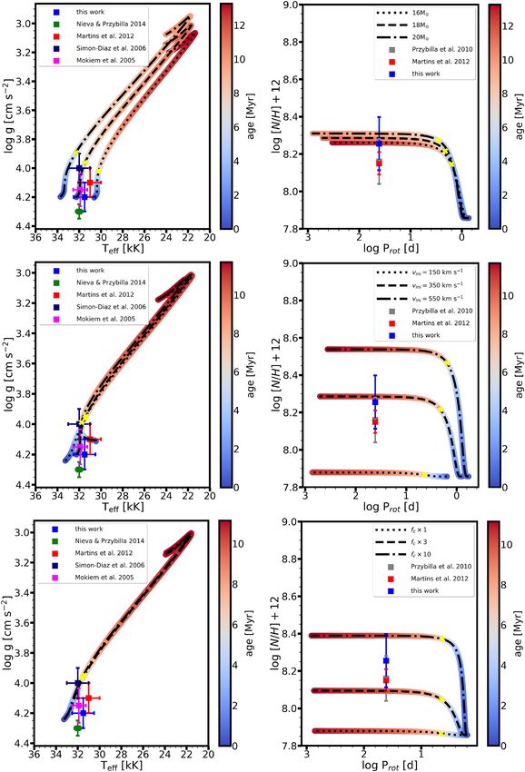
Figure 3. Upper panels: same as Fig. 2 but with Mini = 18 M and adopting fast rotation with ini = 550 km s−1 while varying the braking efficiency. Middle
panels: with Mini = 18 M and ini = 250 km s−1 , fc = 0.33 and fMB = 10 (dotted), and ini ≈ 550 km s−1 , fc = 0.1 and fMB = 10 (dashed). Lower panel:
14 N/12 C mass fraction as a function of 14 N/16 O mass fraction. The derived CNO abundance ratios are shown with blue marker. The evolutionary models (same
as in the middle panels) which can mix core material to the surface evolve towards the top right of the diagram. The end point of the model is where surface
rotation is slow enough (Prot ≈10 d, see middle panel) that the surface abundance does not change anymore. Since this is reached in about the first 2–3 Myr, the
further time evolution leads to no changes on this diagram.
MNRAS 504, 2474–2492 (2021)2482 Z. Keszthelyi et al.
scenarios are practically identical to a (perhaps more commonly Zahn (1992), the latter two are combined into one effective diffusion
known) flux decay scenario. Contrasted with the flux conservation coefficient, Deff (see Meynet et al. 2013 and references therein). In
scenario (equation 3), we now have: this work, we test two prescriptions. In one case (which will be
referred to as D11 hereafter), the shear is adopted from Maeder
F ∝ Bsurf (t) R2 (t) = Bsurf (t = 0) exp (−fdec t/τ ) R2 (t) . (5)
(1997) as
In Fig. 4, models with different magnetic field evolution scenarios 2
are shown. The top panels show models with magnetic flux conserva- Hp K 9π d ln
Dshear = , (6)
tion (equation 3), whereas the middle and lower panels show models gδ ϕδ ∇μ + (∇ad − ∇rad ) 32 d ln r
with magnetic field decay (equations 4–5).
With magnetic field evolution, the models can have an initially where Hp is the local pressure scale height, g is the local gravitational
stronger magnetic field and consequently initially more efficient acceleration, δ and ϕ are derivatives from the equation of state, K is
magnetic braking. Although time dependent, this is somewhat similar the thermal diffusivity, is the angular velocity, and r is the distance
to the previous tests where fMB was used to obtain a more efficient from the centre. The horizontal turbulence is adopted from Zahn
Downloaded from https://academic.oup.com/mnras/article/504/2/2474/6195517 by guest on 24 October 2021
magnetic braking. This means that magnetic field evolution, in (1992) as
principle, allows for adopting a higher initial rotational velocity and
thus a higher initial (‘natural’) efficiency of rotational mixing. Dh = r|2V (r) − αU (r)| , (7)
Assuming magnetic flux conservation, a field with an initial
2
strength of 1 kG (assumed dipolar) well approximates the present- where α = 12 d ln(r
d ln r
)
and U(r) and V(r) are the horizontal and vertical
day field strength of τ Sco, however, leads to a small impact in its components of the meridional circulation.
overall evolution compared to the reference model (600 G polar field In the second case (which we will refer to as D22 hereafter), the
strength constant in time). An initial 4 kG field produces efficient shear is adopted from Talon & Zahn (1997) as
braking albeit no nitrogen enrichment. This model also leads to a
2
magnetic field strength over the entire evolution (except close to the Hp K + Dh 9π d ln
TAMS) which is far too strong (> 1 kG) to be compatible with Dshear = ,
gδ ϕ ∇μ 1 + K + (∇ad − ∇rad ) 32 d ln r
spectropolarimetric measurements (see Appendix B). δ Dh
When magnetic field decay is considered, the model with an initial (8)
3 kG field strength (assumed dipolar) and decay efficiency fdec of
unity produces sufficient nitrogen excess, however, does not spin- and the horizontal turbulence is adopted from Maeder (2003) as
down fast enough (middle panels). The model with an initial 9 kG
field strength does produce efficient braking, and while the long Dh = Ar (r(r)V (r)|2V (r) − αU (r)|)1/3 , (9)
rotation period is recovered, no mixing is achieved. Increasing the
mixing efficiency in this model by a factor of 3 leads to an acceptable, where A = (3/400nπ )1/3 with n being the number of axial rotations
self-consistent match with the observables of τ Sco. However, the (Maeder 2003).
observable field strength would remain above 3 kG in the first 6 Myr, Angular momentum transport is modelled by using an advecto-
which is at odds with the observations. diffusive equation which accounts for the radial component of
Experiments with 30 kG initial field strengths allow to reproduce meridional currents (the advective term) and shears (the diffusive
the current long rotation period (lower panels). Increasing fc by a term). The meridional currents are an advective process by nature.
factor of 10 is required to reach nitrogen excess. However, a decay The shear term is modified when using the D11 (Dshear adopted
efficiency of 2 still yields a magnetic field strength well above 1 kG from Maeder 1997) or D22 (Dshear adopted from Talon & Zahn
in 6 Myr. fdec = 4 results in an acceptable self-consistent solution. 1997) schemes in the models. Both of these cases, without internal
From these tests, we conclude that while magnetic field evolution magnetic fields, allow for radial differential rotation and lead to a
can, to some extent, alleviate the large magnetic braking efficiency weaker core-envelope coupling than in solid-body rotating models.
(fMB = 10) that was needed in the model with a constant 600 G field We do not test solid-body rotating models here because it was shown
strength, it faces the challenge to reach a sufficiently low, sub-kG in previous works that it leads to less surface enrichment than dif-
field strength in 6 Myr. This requires a high magnetic field decay ferentially rotating models (Meynet, Eggenberger & Maeder 2011,
efficiency. Importantly, in all tests, the need for a more efficient Paper I).
chemical mixing is still present. The effects of the surface magnetic field are modelled via magnetic
braking, which is implemented as a boundary condition for internal
angular momentum transport (Meynet et al. 2011; Georgy et al.
3.3 GENEC modelling: setup
2017, Paper I , Paper II). We refer the reader to Paper II Appendix B,
In GENEC, we adopt similar modelling assumptions as Ekström et al. where the MESA and GENEC implementations of magnetic braking
(2012). A solar metallicity of Z = 0.014 is used with the Asplund are detailed and contrasted. Since in GENEC only the outermost
et al. (2009) mixture of metals except for neon (Ekström et al. 2012), layers are ascribed to lose specific angular momentum, the use of
and isotopic ratios are from Lodders (2003). The adopted mixing angular momentum transport without a strong coupling means that
efficiency in the convective core is α MLT = 1.6. A step overshooting significant shears can develop in the outer part of the stellar envelope,
method is applied with α ov = 0.1. The opacity tables are adopted while meridional currents remain efficient to transport chemical
from OPAL (Rogers & Iglesias 1992). Mass-loss rates are calculated elements close to the stellar core. (Note that in MESA, we model
following the prescription of Vink, de Koter & Lamers 2000 and the opposite scenario: shears remain efficient close to the core but
Vink et al. 2001, multiplied by a factor of 0.85. (weak) meridional circulation dominates the transport in the outer
Chemical element transport is modelled as a diffusive process envelope.) The equatorial magnetic field strength is set to Beq =
(Pinsonneault et al. 1989), adding up from three terms: vertical 300 G (corresponding to 600 G polar) and is kept constant over
shear, horizontal turbulence, and meridional currents. Following time.
MNRAS 504, 2474–2492 (2021)The effects of surface fossil magnetic fields on massive star evolution – III 2483
Downloaded from https://academic.oup.com/mnras/article/504/2/2474/6195517 by guest on 24 October 2021
Figure 4. MESA models with Mini =18 M and ini > 500 km s−1 are shown. Upper panels: Models with magnetic flux conservation compared to the reference
model (Bp = 600 G). Standard efficiencies are used for fc and fMB . Middle and lower panels: Models with magnetic field decay. The magnetic braking efficiency
is set with fMB = 1 but the decay efficiency fdec and rotational mixing efficiency fc are varied (cf. equations 1 and 4). The two models with initially 8 kG fields
in the middle right-hand panel overlap.
MNRAS 504, 2474–2492 (2021)2484 Z. Keszthelyi et al.
Downloaded from https://academic.oup.com/mnras/article/504/2/2474/6195517 by guest on 24 October 2021
Figure 5. Shown are models computed with the Geneva code on the Kiel (left) and Hunter-P diagrams (right). The colour-coding scales with stellar age. Yellow
crosses indicate an age of 6 Myr.
3.4 GENEC modelling: results and analysis the model predictions typically yield notable surface enrichment in
the second half of the main sequence only.
Some of the major differences between GENEC and MESA are the
treatment of angular momentum transport and the way magnetic
braking is applied. We seek to probe here whether the same four strict 4 DISCUSSION
observables of τ Sco could be reconciled when using the modelling
assumptions as described above. Here, we do not introduce efficiency We have shown that standard single-star evolutionary models cannot
parameters, instead we test whether a change in mixing prescription simultaneously reproduce the observed log g, Teff , N/H, and Prot of
alone could remedy the discrepancies. τ Sco.
Single-star models matching the observations on the Kiel diagram
(fitting log g and Teff ) can either reproduce the N/H ratio but not the
3.4.1 Impact of initial mass, rotation, and mixing prescription observed rotation, or, inversely can reproduce the observed rotation
but not the surface enrichment. This is precisely the same problem
Fig. 5 shows a reference model (dashed line) with Mini =18 M and encountered by the post-merger models of Schneider et al. (2020).
ini = 300 km s−1 , using the D22 scheme (see above) and assuming a Possible resolutions, in the frame of single-star models, is to
600 G polar field strength constant in time. The colour-coding scales consider a more efficient chemical mixing and/or a more efficient
with the stellar age. When decreasing the initial mass, only modest magnetic braking. The latter one hypothetically could be replaced
differences are seen (primarily, a shift in the effective temperature by a magnetic field decay scenario. Overall, we find that in order to
to lower values). Likewise, when the initial rotational velocity is reconcile all observables of τ Sco, rather extreme assumptions are
increased (by 100 km s−1 here) compared to the reference model, the necessary, which would not be compatible with observations of other
impact remains small. Changing the mixing prescription, however, stars.
leads to a large difference. The model with the D11 scheme allows
for a far more efficient chemical mixing, and due to the increased
mean molecular weight on average inside the star, a more vertical 4.1 Chemical mixing
evolution on the Kiel diagram.
Rotational mixing in massive stars is presently one of the most
From these model computations, we can conclude that within
uncertain processes influencing stellar evolution. A large number
observational and modelling uncertainty the Kiel diagram predicts
of observations show discrepancies with current model predictions
an age of at most 6 Myr.9 This is at odds with the model ages predicted
(e.g. Hunter et al. 2009; Martins et al. 2017; Cazorla et al. 2017b;
from the Hunter-P diagram where we encounter the same problem
Markova, Puls & Langer 2018).
as before. Namely, sufficient nitrogen enrichment and low spin
Potential sources of these discrepancies are likely many-fold. Im-
velocity are not obtained with a self-consistent solution when using
portantly, stellar evolution model computations remain restricted to a
standard formulas for chemical mixing and magnetic braking. This
1D treatment. Therefore, necessarily, scaling factors are introduced to
is consistent with findings of Meynet et al. 2011 and Paper I , where
model chemical mixing (Pinsonneault et al. 1989) and some mixing
prescriptions are derived based on order-of-magnitude estimates
9 The values obtained from Simón-Dı́az et al. (2006) may allow for a somewhat (Brott et al. 2011). Even more, the relevant physical processes and
higher age, although the values we derive in this study would point to a lower their interactions are not yet fully understood (e.g. Maeder 2009) and
age and perhaps very slightly lower initial mass than 17 M , based on the some processes are not yet ubiquitously modelled and included in the
GENEC models. computations, such as mixing by internal gravity waves (Decressin
MNRAS 504, 2474–2492 (2021)The effects of surface fossil magnetic fields on massive star evolution – III 2485
et al. 2009; Mathis et al. 2013; Rogers et al. 2013; Aerts & Rogers The evolution of surface fossil magnetic fields remains largely
2015; Rogers & McElwaine 2017; Bowman et al. 2019a,b, 2020). uncertain. Several observational studies are consistent with magnetic
Despite the notable uncertainties, a drastic increase in the effi- flux conservation, whereas other empirical evidence points to a more
ciency of the present-day prescriptions of rotational mixing by a rapid decline in field strength over time, suggesting a flux decay
factor of 3 (in the initially fast-rotator MESA model) or a factor of scenario (see Paper I and Paper II , and references therein).
10 (in the initially moderate-rotator MESA model) seem excessive From a theoretical standpoint, fossil fields are expected to slowly
in a single-star model. We estimate that (along with an increase in dissipate on an Ohmic time-scale, given by the induction equation of
magnetic braking efficiency) a similar increase in chemical mixing non-ideal MHD:
would also be required in the ‘D11’ GENEC model to obtain a self- ∂B
consistent solution. η∇ 2 B = , (10)
∂t
Let us recall here that the chemical mixing efficiency in rotating
where η is the magnetic diffusivity (assumed to be constant in space),
stellar evolution models is calibrated such that with an initial mean
B is the magnetic field vector, t is the time, and we assume that the
rotation rate, they reproduce the mean surface nitrogen abundances
fluid velocity is zero, accounting for an equilibrium fossil magnetic
Downloaded from https://academic.oup.com/mnras/article/504/2/2474/6195517 by guest on 24 October 2021
of B-type stars at the end of the main sequence phase (e.g. Brott et al.
field (Braithwaite & Spruit 2017).
2011). If we change this mixing efficiency for the purpose of fitting
For a fully ionized plasma, the diffusion time-scale can be
the data of τ Sco, then an appropriate physical reason should be given.
approximated as the ratio of the square of a characteristic length
At the moment, we are unaware of a physical cause which could be
scale and the magnetic diffusivity:
invoked in the single-star channel. Nevertheless, adopting a factor
of 10 increase is not unprecedented in evolutionary modelling, for R2
example, Aguilera-Dena et al. (2020) use such an increased mixing tdiff ∼ . (11)
η
efficiency in their approach.
For the Sun and low-mass stars, this formula typically leads to
Interestingly, τ Sco stands out from the sample of magnetic mas-
estimates of diffusion time-scales longer than the main sequence
sive stars as being a putative blue straggler. Blue stragglers are often
lifetime (e.g. Cowling 1945; Feiden & Chaboyer 2014). Here, we
associated with stellar mergers or quasi-chemically homogeneously
refrain from providing an estimate for more massive stars (and
evolving stars. Although quasi-chemically homogeneous evolution
τ Sco in particular) since the uncertainty in an appropriate magnetic
via long-term rapid rotation may help explain the surface enrichment
diffusivity is several orders of magnitudes (e.g. Charbonneau &
of τ Sco, it is unclear if at all the star could suddenly become a very
MacGregor 2001). Since the outward diffusion of the magnetic flux
slow rotator as observed, therefore this evolutionary channel does
is a possible mechanism to explain why flux decay may need to
not seem very favourable. Magnetic OB stars are typically found to
be invoked as a field evolution scenario, in this case, we would
be consistent with a usual ‘redward’ evolution after their initial spin-
require the diffusion time-scale to be shorter than the ∼12 Myr
down (Paper I and Paper II). Furthermore, being a magnetic blue
main sequence lifetime of our models. In conclusion, the scenario of
straggler poses the interesting question whether all blue stragglers
magnetic flux decay still requires rigorous theoretical considerations
would have a detectable magnetic field. Schneider et al. (2016)
(Braithwaite & Spruit 2017).
suggested that since the merger rate may be higher in blue stragglers,
The magnetic braking formula by ud-Doula et al. (2009) is robust
consequently the incidence rate of magnetism may also be higher.
but relies on important assumptions such as the field geometry and
However, observational efforts dedicated to hot stars have not found
alignment with the rotation axis. In principle, the complexity of
such hints yet (Mathys 1988; Grunhut et al. 2017).
τ Sco’s magnetic field geometry is expected to decrease, and not
Morel et al. (2008), Aerts et al. (2014), and Martins et al. (2012),
increase, the spin-down efficiency since the lowest order harmonic
Martins et al. (2015) analysed the nitrogen enrichment of magnetic
(i.e. the dipole component) has the most relevant contribution to spin-
OB stars and identified a number of cases with nitrogen excess
down. Nevertheless, the impact of a strong azimuthal field remains
(including τ Sco). Presently, it remains elusive why some stars show
uncharacterized. Recent simulations (ud Doula et al., in preparation)
excess and others do not. In Paper I, we proposed that the observable
show that oblique rotation does not significantly affect the spin-down
nitrogen enrichment of magnetic stars largely depends on presently
scaling either.10
unconstrained mixing processes (and their efficiencies), therefore
the outcome is a multivariate function of a number of parameters
(Aerts et al. 2014; Maeder et al. 2014), and not only a function of the 4.3 Alternative evolutionary scenarios
magnetic field strength.
Although the single-star and the merger scenario have been suggested
to explain the observables of τ Sco, nature may potentially offer
4.2 Magnetic field evolution and spin-down different ways to explain them.
Regarding its magnetic field characteristics, τ Sco clearly stands Two main channels might be considered. i) Higher mixing effi-
out of the known non-chemically peculiar magnetic B-type stars ciency may be induced by a close companion star. Recent works
(this sample is discussed by Shultz et al. 2019b and confronted with have indeed shown that tidally induced mixing can supersede the
evolutionary models in Paper II). The complexity of τ Sco’s magnetic efficiency compared to a single star (e.g. Song et al. 2013). This
field is unique. In general, a dipole-dominated model allows for would require the presence of a main sequence companion star (see
reproducing magnetic field measurements (even if other higher order below). ii) The surface enrichment of τ Sco might have been caused
harmonics are present), although a number of cases indeed point to a by an earlier mass-transfer event from a more massive companion
quadruple-dominated geometry (Shultz et al. 2018, 2019a). Recently,
David-Uraz et al. (2021) found that NGC 1624 - 2’s magnetic field is 10 Deviations in the rate of angular momentum loss by approximately up
more complex than the typically assumed pure dipole. This evidence to 30 per cent can be reached for oblique rotators (ud Doula, private
suggests that deviations from the pure dipole geometry may not be communication). However, these deviations are expected to decrease the
uncommon but require extensive monitoring to identify it. rate of angular momentum loss.
MNRAS 504, 2474–2492 (2021)You can also read