Development of novel hybridized models for urban flood susceptibility mapping - Nature
←
→
Page content transcription
If your browser does not render page correctly, please read the page content below
www.nature.com/scientificreports
OPEN Development of novel hybridized
models for urban flood
susceptibility mapping
Omid Rahmati1,2*, Hamid Darabi3, Mahdi Panahi4,5, Zahra Kalantari6, Seyed Amir Naghibi7,
Carla Sofia Santos Ferreira8, Aiding Kornejady9, Zahra Karimidastenaei3,
Farnoush Mohammadi10, Stefanos Stefanidis11, Dieu Tien Bui12,13* & Ali Torabi Haghighi3
Floods in urban environments often result in loss of life and destruction of property, with many
negative socio-economic effects. However, the application of most flood prediction models still
remains challenging due to data scarcity. This creates a need to develop novel hybridized models
based on historical urban flood events, using, e.g., metaheuristic optimization algorithms and wavelet
analysis. The hybridized models examined in this study (Wavelet-SVR-Bat and Wavelet-SVR-GWO),
designed as intelligent systems, consist of a support vector regression (SVR), integrated with a
combination of wavelet transform and metaheuristic optimization algorithms, including the grey wolf
optimizer (GWO), and the bat optimizer (Bat). The efficiency of the novel hybridized and standalone
SVR models for spatial modeling of urban flood inundation was evaluated using different cutoff-
dependent and cutoff-independent evaluation criteria, including area under the receiver operating
characteristic curve (AUC), Accuracy (A), Matthews Correlation Coefficient (MCC), Misclassification
Rate (MR), and F-score. The results demonstrated that both hybridized models had very high
performance (Wavelet-SVR-GWO: AUC = 0.981, A = 0.92, MCC = 0.86, MR = 0.07; Wavelet-SVR-Bat:
AUC = 0.972, A = 0.88, MCC = 0.76, MR = 0.11) compared with the standalone SVR (AUC = 0.917,
A = 0.85, MCC = 0.7, MR = 0.15). Therefore, these hybridized models are a promising, cost-effective
method for spatial modeling of urban flood susceptibility and for providing in-depth insights to guide
flood preparedness and emergency response services.
Floods are the most widespread and damaging natural disaster, imposing a range of adverse effects across coun-
tries and regions all over the w
orld1. These include fatalities, displacement of people, damage to infrastructure,
and environmental damage, thus affecting economic activities and d evelopment2,3. In 2006–2015, floods were
the leading cause of disaster deaths in African regions, in Central and South America and in Central, S outh4,
and West A sia5. In 2016, worldwide floods affected ~ 78 million people and caused 4,731 fatalities and damage
1
Geographic Information Science Research Group, Ton Duc Thang University, Ho Chi Minh City, Viet Nam. 2Faculty
of Environment and Labour Safety, Ton Duc Thang University, Ho Chi Minh City, Viet Nam. 3Water, Energy
and Environmental Engineering Research Unit, University of Oulu, Oulu, Finland. 4Geoscience Platform
Research Division, Korea Institute of Geoscience and Mineral Resources (KIGAM), 124, Gwahak‑ro, Yuseong‑gu,
Daejeon 34132, Republic of Korea. 5Division of Science Education, Kangwon National University, Chuncheon‑si,
Gangwon‑do 24341, Republic of Korea. 6Department of Physical Geography and Bolin Centre for Climate
Research, Stockholm University, Stockholm, Sweden. 7Department Water Resources Engineering and Center for
Middle Eastern Studies, Lund University, Lund, Sweden. 8Research Centre for Natural Resources, Environment
and Society (CERNAS), Polytechnic Institute of Coimbra, Agrarian School of Coimbra, Coimbra, Portugal. 9Spatial
Sciences Innovators, Consulting Engineering Company, Tehran, Iran. 10Department of Arid and Mountainous
Regions Reclamation, Faculty of Natural Resources, University of Tehran, Tehran, Iran. 11Laboratory of
Mountainous Water Management and Control, Faculty of Forestry and Natural Environment, Aristotle University of
Thessaloniki, Thessaloniki, Greece. 12Institute of Research and Development, Duy Tan University, 550000 Da Nang,
Viet Nam. 13Geographic Information System group, Department of Business and IT, University of South-Eastern
Norway, 3800 Bø i Telemark, Norway. *email: omid.rahmati@tdtu.edu.vn; buitiendieu@duytan.edu.vn
Scientific Reports | (2020) 10:12937 | https://doi.org/10.1038/s41598-020-69703-7 1
Vol.:(0123456789)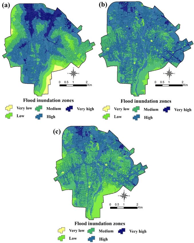
www.nature.com/scientificreports/
costing 60 billion USD5. Asia is the most vulnerable continent6, with floods being responsible for ~ 90% of all
human losses due to natural hazards on that c ontinent7,8.
Urban floods often cause loss of life and other health impacts such as damaging the living environment, pollu-
tion of drinking water, and outbreaks of diseases such as hepatitis E, gastrointestinal disease, and l eptospirosis9,10.
Floods in urban areas can be triggered by intensive rainfall, rapid snowmelt, and rises in water level (e.g., sea,
river, lake, and groundwater)11,12. Also, physical location, rapid urban expansion, and land-use change have a
significant effect on flood occurrences4. Although the extensive implementation of flood control measures, such
as widespread grey infrastructures (e.g., dams and channelization) and nature-based solutions (e.g., wetlands and
bioswales), most cities around the world remain vulnerable to flood h azards13. Low capacity of urban drainage
systems can increase the inundation area and decrease the efficiency of infrastructures, and consequently, exac-
erbate the risk of urban floods3. Climate change and urbanization may increase the frequency and magnitude
of urban flood events.
The frequency of flood-related disasters is projected to increase in the future due to the growing global
population, particularly in developing countries, increased soil sealing as a result of urbanization, and climate
change14,15. In Europe, for example, floods due to climate change are expected to affect three-fold more people
in 2050 than in the current climate and to cause damage costing €20–40 billion16. Lack of financial resources,
particularly in developing countries, may represent an additional challenge in flood prevention and preparation
for floods17.
Since floods are a natural phenomenon that cannot be prevented (2007/60/EC), implementation of flood
management strategies is necessary. Flood reduction, one of the key societal challenges of this c entury15, relies on
prior flood risk assessment, which includes flood hazard maps showing potentially affected areas under different
flood scenarios (i.e., frequency and magnitude). Several methodologies based on numerical models (statistical
relationships between hydrological input and output) and physically-based models (relationships between rainfall
and runoff) and techniques (e.g., remote sensing and geographic information system, GIS) have been used to
generate flood hazard maps in urban a reas8,18. However, the accuracy of these maps is affected by (i) nonlinear
dynamic characteristics of floods, as a result of distinct factors such as precipitation and human a ctivities19; (ii)
limitations in data availability, including detailed hydrological and hydraulic data, particularly in developing
countries, despite advances provided by new remote sensing techniques, such as satellites, multisensory systems,
and/or radar11; and (iii) limited applicability of methods at different s cales20. These drawbacks have encouraged
the use of advanced data-driven models, e.g., machine learning (ML), a field of artificial intelligence that uses
computer algorithms to analyze and predict information through learning from training d ata21.
In recent years, ML has been used by hydrologists for flood susceptibility mapping11, e.g., based on novel
algorithms to improve river discharge e stimation22, or new models built upon past flood inventory maps and
including a number of flood conditioning factors19. Flood inundation is significantly influenced by a wide range of
factors such as s lope23, land u se10, distance from r iver3, drainage-system c apacity11, distance to c hannel11, and land
subsidence6,24; therefore, ML models should be able to identify relationships between flood inundation events and
these factors. Some of the most popular methods for flood susceptibility mapping are Decision T rees25, Artificial
Neural Networks10, and Support Vector Machines (SVM)19. Among these methods, SVM is becoming increas-
ingly well-known19. It is a class of support vector, a search algorithm using statistical learning theory, which is
used to minimize over-fitting and reduce the expected error of learning machines26. It has also been extended
as a regression tool, called Support Vector Regression (SVR)27. SVMs are suitable for both linear and nonlinear
classification and are efficient and reliable tools for producing flood susceptibility maps in a GIS e nvironment19.
Machine learning methods show better performance and provide more cost-effective flood susceptibility
assessments than numerical and physical methods22,26. However, their performance may differ from one region
to another, due to different geo-environmental factors8, the complex algorithms they contain, which sometimes
make interpretation d ifficult26, and/or their structural limitations, such as the requirement for a large number of
parameters, which can impair wider applications and compromise model performance3. Therefore, a major trend
in advancing flood susceptibility predictions based on the determination of flood-prone regions is hybridiza-
tion, i.e., integration of two or more ML methods, such as Adaptive Neuro-Fuzzy Interface Systems (ANFIS)8,
integration between ML and more conventional methods, and/or soft computing t echniques26. Novel hybrid
methods involving SVR, such as ANFIS-SVR20, Recurrent Neural Network (RNN)-SVR28, Hydrologic Engineer-
ing Center-Hydrologic Modeling System (HEC-HMS)-SVR29, and SVR-Discrete Wavelet Transform (DWT)-
Empirical Mode Decomposition (EMD)30, have achieved notable progress in terms of accuracy, generalization,
uncertainty, performance, and robustness.
Some ML models have been applied in different watersheds (i.e., natural areas) around the w orld3,8,11, but
urban flood susceptibility modeling still remains challenging. The aim of this study was to develop new hybrid-
ized models for urban flood susceptibility mapping by integrating SVR with two metaheuristic optimization
algorithms: (i) Bat and Grey Wolf Optimizer (GWO) and (ii) the wavelet transform concept. As a study case, the
novel hybridized models (Wavelet-SVR-Bat and Wavelet-SVR-GWO) and standalone SVR model were applied
to Amol city, in northern Iran, and their results were compared using different cutoff-dependent and cutoff-
independent evaluation criteria. Production of accurate flood susceptibility maps is essential to support decision-
making on developing resilience planning, emergency responses, and flood mitigation.
Description of the study area. The city of Amol (36°26′–36°29.5′N, 52°19.6′–52°24′E) is located on the
southern coast of the Caspian Sea, in the west of Mazandaran Province, northern Iran (Fig. 1). The city lies near
the outlet of the Haraz River watershed (about 1,100 km2 in area), with the Haraz river passing through the heart
of Amol city and then reaching the Caspian S ea31. Amol is a rapidly growing and heavily industrialized city, cur-
rently occupying an area of 27.1 km2 and hosting a population of approximately 300,000. Residential areas in the
Scientific Reports | (2020) 10:12937 | https://doi.org/10.1038/s41598-020-69703-7 2
Vol:.(1234567890)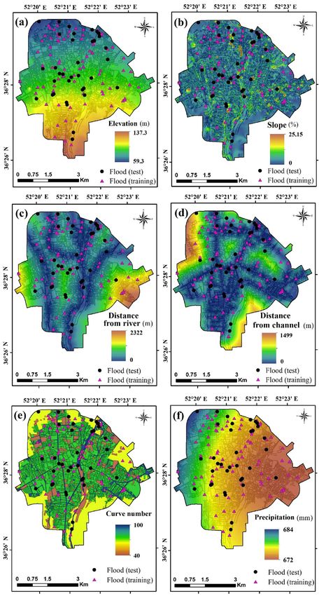
www.nature.com/scientificreports/
Figure 1. Location of Amol city, Mazandaran province, Iran, and sites affected by past floods. The map was
generated using ArcGIS Desktop 10.7.1, https://desktop.arcgis.com/en.
city are mainly surrounded by alluvial plains (agricultural land, orchards) to the north and high mountains (the
Alborz range) covered by forest to the s outh32. The region has a humid climate, with a moderate temperature
(17.4 °C mean annual temperature) and mean annual precipitation of 650 mm (2001–2019), recorded at Amol
weather station of the Iranian Meteorological Organization (IRIMO). Amol city was selected for the present
study due to the many catastrophic floods that have occurred annually in recent years, damaging thousands of
homes and infrastructure, disrupting traffic, trade, and public services, and taking lives. Figure 2 shows some
consequences of previous floods in Amol city.
Results
Multicollinearity analysis. After implementing the variance inflation factors (VIF) and tolerance (TOL)
indices, it was found that there is no critical multicollinearity between the factors, since the values were all placed
within the acceptable range (Table 1).
Goodness‑of‑fit and predictive performance of the models. Cutoff‑independent criteria (AUC
method). The results of goodness-of-fit (i.e., accuracy in the training step) and predictive performance (i.e.,
accuracy in the validation step) of the three models in terms of the AUC metric are displayed in Fig. 3. Based
on the AUC, Wavelet-SVR-Bat had the highest accuracy in training (AUC = 0.986), followed by Wavelet-SVR-
GWO (AUC = 0.984) and the standalone SVR (AUC = 0.949). The goodness-of-fit of each model was measured
based on the data used to calibrate the model, and it shows how well the model fits the training dataset. The
predictive power of the model cannot be judged using the goodness-of-fit of the model, so a separate analysis of
predictive performance was conducted. In terms of predictive performance, Wavelet-SVR-GWO had the highest
accuracy (AUC = 0.981), slightly better than Wavelet-SVR-Bat (AUC = 0.972). The AUC value of the standalone
SVR model in this step was 0.917. Therefore, in order of performance, the ranking was: Wavelet-SVR-GWO,
Wavelet-SVR-Bat, and SVR, although with minor differences.
Scientific Reports | (2020) 10:12937 | https://doi.org/10.1038/s41598-020-69703-7 3
Vol.:(0123456789)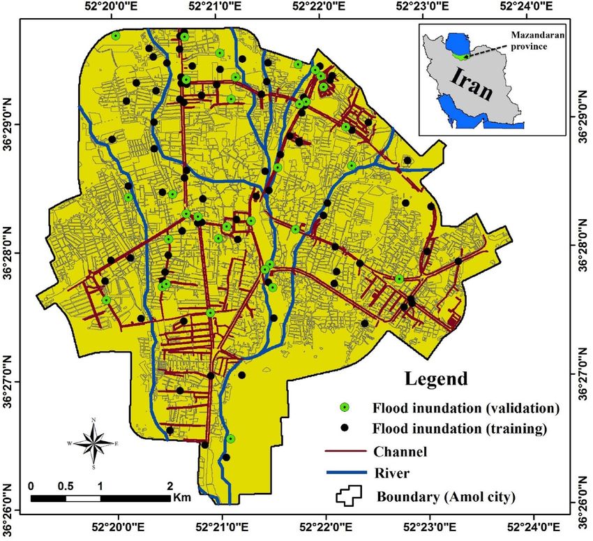
www.nature.com/scientificreports/

                                      Figure 2.  Field photographs of flooded sites in Amol city, taken on March 17, 2019 (photographs by Hamid
                                      Darabi).

                                                                  Collinearity
                                                                  Statistics
                                       Flood-controlling factor   TOL     VIF     Std. error
                                       Elevation                  0.624   1.603   0
                                       Curve number               0.987   1.013   0.002
                                       Distance from river        0.337   2.969   0
                                       Distance from channel      0.445   2.245   0
                                       Precipitation              0.673   1.486   0
                                       Slope percentage           0.919   1.089   0

                                      Table 1.  Variance inflation factor (VIF) and tolerance (TOL) values representing the multicollinearity
                                      between selected flood-controlling factors.

                                      Cutoff‑dependent criteria. The results of accuracy assessment using the cutoff-dependent criteria TPR, FPR,
                                      Accuracy, MCC, F-score, and MR, are summarized in Table 2. These evaluation metrics provided better insights
                                      regarding the accuracy of the three models.
                                          In terms of goodness-of-fit, Wavelet-SVR-GWO was the best model. It had a higher Accuracy (0.951), MCC
                                      (0.903), and F-score (0.951), and also a lower MR (0.048) and FPR (0.037) than other models (Table 1). How-
                                      ever, in terms of the TPR metric, Wavelet-SVR-Bat (0.973) was slightly better than Wavelet-SVR-GWO (0.94).
                                      Importantly, the standalone SVR had the lowest accuracy based on all cutoff-dependent evaluation metrics. As
                                      indicated above, goodness-of-fit only provides insights regarding the degree of fit of data to the model. Therefore,
                                      the prediction capability of the models was investigated in a validation step. The results of the validation analysis
                                      clearly indicated the superior performance of Wavelet-SVR-GWO based on the TPR (1.00), Accuracy (0.926),
                                      MCC (0.861), F-score (0.918), and MR (0.073). It was followed by Wavelet-SVR-Bat, which performed very well
                                      in terms of TPR (0.857), Accuracy (0.882), MCC (0.766), F-score (0.882), and MR (0.117). The standalone SVR
                                      had the lowest accuracy in terms of predictive performance, with TPR of 0.848, FPR of 0.145, Accuracy of 0.852,
                                      MCC of 0.705, F-score of 0.848, and MR of 0.147. In order of performance, the ranking was again: Wavelet-SVR-
                                      GWO, Wavelet-SVR-Bat, and SVR.

                                      RMSE metric. Figure 4 shows the target and outputs of the SVR model for the (a) training and (b) validation
                                      datasets, and (c, e) the mean squared error (MSE) and root mean square error (RMSE) values for these datasets.
                                      As can be seen, MSE and RMSE values of 0.087 and 0.295 were obtained for SVR in predicting the training set,

          Scientific Reports |   (2020) 10:12937 |                  https://doi.org/10.1038/s41598-020-69703-7                                           4

Vol:.(1234567890)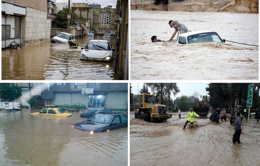
www.nature.com/scientificreports/

                            Figure 3.  Goodness-of-fit and predictive performance of models based on the AUC metric: (a) SVR in training,
                            (b) SVR in validation, (c) Wavelet-SVR-Bat in training, (d) Wavelet-SVR-Bat in validation, (e) Wavelet-SVR-
                            GWO in training, and (f) Wavelet-SVR-GWO in validation.

                                                     Goodness-of-fit (training step)                Predictive performance (validation step)
                             Evaluation criteria     SVR     Wavelet-SVR-Bat      Wavelet-SVR-GWO   SVR     Wavelet-SVR-Bat     Wavelet-SVR-GWO
                             TPR (sensitivity)       0.864   0.973                0.940             0.848   0.857               1.000
                             FPR (1 − specificity)   0.142   0.109                0.037             0.145   0.090               0.125
                             Accuracy (A)            0.860   0.927                0.951             0.852   0.882               0.926
                             MCC                     0.721   0.858                0.903             0.705   0.766               0.861
                             F-score                 0.858   0.923                0.951             0.848   0.882               0.918
                             MR                      0.139   0.072                0.048             0.147   0.117               0.073

                            Table 2.  Goodness-of-fit and predictive performance of models based on cutoff-dependent criteria. TPR true
                            positive rate, FPR false positive rate, MCC Matthews correlation coefficient, MR misclassification rate.

                            while MSE and RMSE values of 0.091 and 0.302 were obtained in predicting the validation set. Mean frequency
                            of errors for the training and validation datasets was 0.006 and 0.032, respectively (Fig. 4d,f).
                                Figure 5 shows the accuracy of the Wavelet-SVR-BAT model based on the MSE and RMSE metrics. As can
                            be seen from Fig. 5c, MSE and RMSE values of 0.066 and 0.258 were obtained for Wavelet-SVR-BAT in predict-
                            ing the training set, while it had MSE and RMSE values of 0.068 and 0.251 in the validation step (Fig. 5e). Mean
                            frequency of errors for the training and validation datasets was 0.030 and 0.026, respectively (Fig. 5d,f).
                                Figure 6 indicates the goodness-of-fit and predictive performance of the Wavelet-SVR-GWO model based
                            on the MSE and RMSE metrics. As shown in Fig. 6c,e, Wavelet-SVR-GWO had MSE and RMSE values of 0.057
                            and 0.240 in the training step, and MSE and RMSE values of 0.055 and 0.236 in predicting the validation set.
                            Mean frequency of errors for the training and validation datasets was 0.040, and 0.040, respectively (Fig. 6d,f).
                                According to the results, Wavelet-SVR-GWO and Wavelet-SVR-BAT had lower MSE and RMSE values than
                            the standalone SVR model. Therefore, Wavelet-SVR-GWO can be regarded as the best model (of the three) for
                            spatially modeling flood susceptibility in urban areas.

Scientific Reports |   (2020) 10:12937 |                     https://doi.org/10.1038/s41598-020-69703-7                                                5

                                                                                                                                                  Vol.:(0123456789)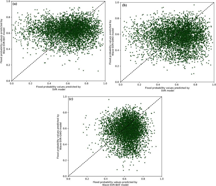
www.nature.com/scientificreports/
Figure 4. (a) Target and output SVR value of training data samples, (b) target and output SVR value of testing
data samples, (c) mean squared error (MSE) and RMSE value of training data samples, (d) frequency of errors
for training data samples, (e) MSE and RMSE value of testing data samples, and (f) frequency of errors for
testing data samples.
Figure 5. (a) Target and output Wavelet-SVR-BAT value of training data samples, (b) target and output
Wavelet-SVR-BAT value of testing data samples, (c) mean squared error (MSE) and root mean square error
(RMSE) of training data samples, (d) frequency of errors for training data samples, (e) MSE and RMSE value of
testing data samples, and (f) frequency of errors for testing data samples.
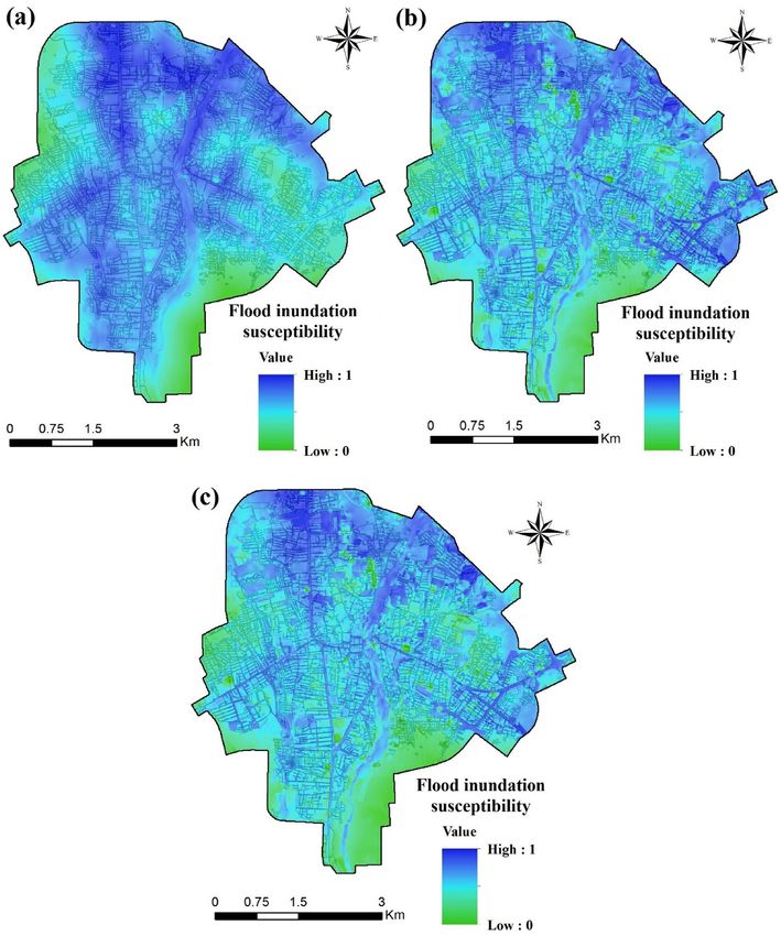
Urban flood susceptibility maps. Figure 7 shows the urban flood susceptibility maps for Amol city
obtained using the SVR, Wavelet-SVR-Bat, and Wavelet-SVR-GWO models. In this example, urban flood sus-
ceptibility is used as a reference to estimate the risk of an area being inundated in any one year in the future.
Areas depicted in blue have higher inundation susceptibility, whereas areas in green have lower, with higher
susceptibility indicating a higher spatial potential for inundation. The maps of the study area generated by the
hybridized models (Fig. 7b,c) showed a similar overall spatial pattern, with high flood probability in the northern
part of the study area. However, there were apparent differences between the results of hybridized models and
the standalone SVR, which showed higher flood susceptibility affecting larger areas, including those surround-
ing the river and the channels dispersed within the city. According to the SVR model, 11.7% of the city falls in the
very high flood inundation susceptibility class, whereas with Wavelet-SVR-Bat and Wavelet-SVR-GWO models
this class covers only 3.4% and 2.4%, respectively, of Amol (Table 3). However, all the models showed high flood
susceptibility for the majority of the study area (affected area ranged from 40.7 to 62.3% with different models).
Figure 8 shows flood inundation zone maps for the city of Amol, created using the SVR, Wavelet-SVR-Bat,
and Wavelet-SVR-GWO models. In the SVR model, 44.8% of the area belongs to the high flood inundation zone,
29.5% medium, 11.7% very high, 11.3% low, and 2.7% very low zones. The results of the Wavelet-SVR-Bat model
Scientific Reports | (2020) 10:12937 | https://doi.org/10.1038/s41598-020-69703-7 6
Vol:.(1234567890)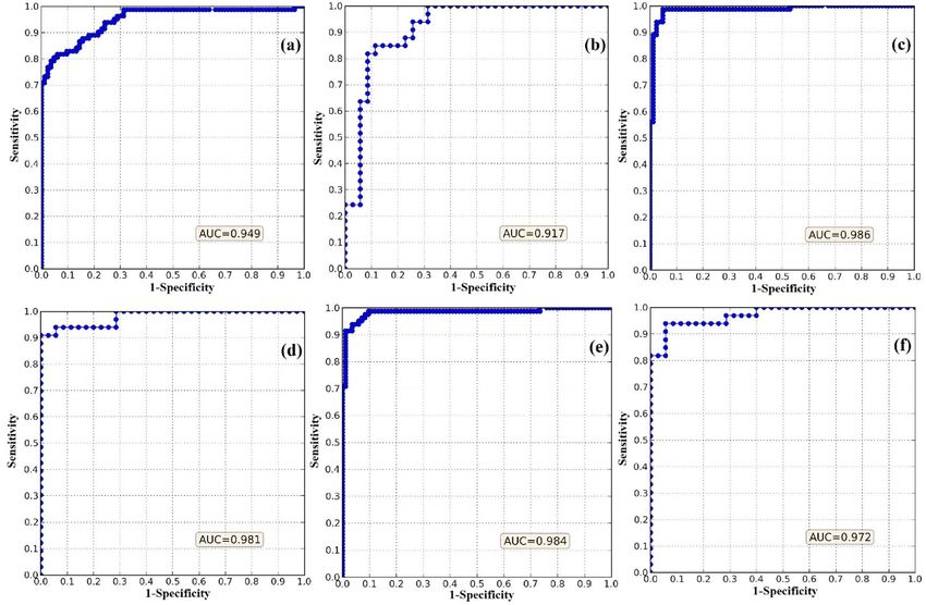
www.nature.com/scientificreports/

                            Figure 6.  (a) Target and output Wavelet-SVR-GWO value of training data samples, (b) target and output
                            Wavelet-SVR-GWO value of testing data samples, (c) mean squared error (MSE) and root mean square error
                            (RMSE) value of training data samples, (d) frequency of errors for training data samples, (e) MSE and RMSE
                            value of testing data samples, and (f) frequency of errors for testing data samples.

                            indicated that the majority of the area (62.3%) belongs to the high flood inundation zone, followed by medium
                            (31.9%), very high (3.4%), low (2.2%), and very low (0.2). The results of the Wavelet-SVR-GWO model showed
                            that approximately 2.4%, 40.7%, 45.7%, 10.9%, and 0.3% of the study area belongs to very high, high, medium,
                            low and very low flood inundation zones, respectively (Fig. 8c).
                                When the flood susceptibility maps prepared with Wavelet-SVR-GWO and Wavelet-SVR-Bat were compared
                            with flood inundation locations in the past, it was found that there was excellent agreement between them. Two
                            schools in Amol are located within zones with a high and very high risk of flood inundation (in the northern part
                            of the study area), which results in children being exposed to urban flood inundation. As discussed by Alderman
                            et al.9, child health in flooded areas must be better reflected in flood mitigation and preparedness programs.

                            Comparison of model predictions. In order to assess spatial agreement between the models, a pairwise
                            agreement plot (PAP) was used. A self-explanatory graphical presentation of the results for the three models is
                            provided in Fig. 9. Unlike a number of quantitative indices that are merely based on metaheuristic classifications
                            and have been repeatedly used for assessing spatial agreement (e.g., kappa), PAP provides more information
                            about the overall agreement and about the data distribution associated with such agreement or disagreement.
                            The dataset includes all the susceptibility values derived from each spatial model, featured as points and ranging
                            from 0 to 1. The diagonal reference line (i.e., 1:1 line) represents the degree to which the models show agreement,
                            meaning that the closer the points get to the 1:1 line, the stronger their spatial agreement. A diagonal distribution
                            of points close to the reference line is ideal, as it represents two perfectly identical susceptibility maps. However,
                            it is normally not achieved since different mathematics produces different susceptibility patterns.
                                 Since the same core mathematical architecture (i.e., SVR) was used in the three models investigated in this
                            study, a certain degree of agreement was achieved, as expected. Figure 9a, comparing the predictions from SVR
                            and Wave-SVR-BAT models, reveals a relatively high dispersion level between selected points. Figure 9b, com-
                            paring the SVR and Wave-SVER-GWO models, shows the highest dispersion among the models. Intuitively,
                            these plots make some inferences regarding the divergence of hybridized algorithms from their core architecture
                            (SVR), based on which divergence appears to be higher for the Wavelet-SVR-GWO hybrid, while Wavelet-SVR-
                            Bat has slightly better agreement with its core. In contrast, in Fig. 9c, focusing on the susceptibility maps of the
                            Wavelet-SVR-Bat and Wavelet-SVR-GWO models, the point cloud seems to be intensely distributed around the
                            reference line and mainly corresponds to values ranging from 0.6 to 0.8 (less dispersed values spreading above
                            0.5), indicating that these two hybridized models have a stronger spatial agreement. Note that these plots do not
                            have connotations of validity and that the inferences refer only to the spatial agreement level. The values above
                            and below the reference line do not signify any superiority, as they may have been overestimated by one model
                            or underestimated by the other.

                            Importance of flood conditioning factors. The relative importance of flood conditioning factors based
                            on the SVR, Wavelet-SVR-Bat, and Wavelet-SVR-GWO models is summarized in Table 4. According to all three
                            models, distance from the channel, distance from river, and curve number are the most important flood condi-
                            tioning factors in the study area. It is reasonable because most floods in the area occur near channels and rivers,
                            where the curve number is considerable (CN > 70). Slope and elevation factors made a moderate contribution to
                            the modeling process, based on all three models. Precipitation showed the lowest importance among all factors.
                            This is probably due to the small spatial variation in the precipitation layer in Amol city. It is in agreement with
                            spatial analysis of flooding events (i.e., observations) in the study area, as demonstrated in Fig. 2, which shows

Scientific Reports |   (2020) 10:12937 |               https://doi.org/10.1038/s41598-020-69703-7                                               7

                                                                                                                                           Vol.:(0123456789)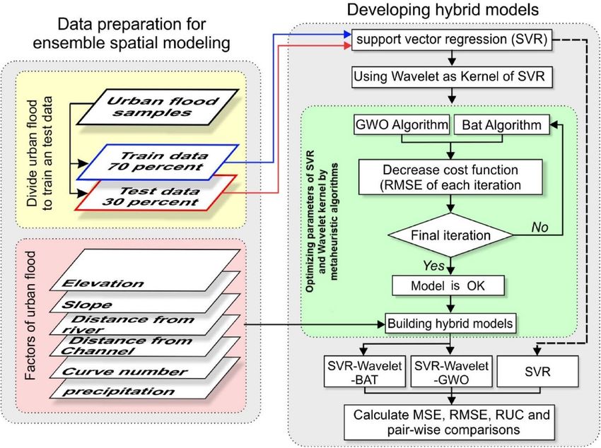
www.nature.com/scientificreports/
Figure 7. Flood inundation susceptibility maps for the city of Amol according to: (a) the SVR model, (b) the
Wavelet-SVR-Bat model, and (c) the Wavelet-SVR-GWO model. These maps were generated using ArcGIS
Desktop 10.7.1, https://desktop.arcgis.com/en/.
Flood inundation classes
Model type Model name Very low Low Medium High Very high
Standalone SVR 2.7 11.3 29.5 44.8 11.7
Wavelet-SVR-Bat 0.2 2.2 31.9 62.3 3.4
Hybridized models
Wavelet-SVR-GWO 0.3 10.9 45.7 40.7 2.4
Table 3. Relative distribution of flood inundation classes from different models.
Scientific Reports | (2020) 10:12937 | https://doi.org/10.1038/s41598-020-69703-7 8
Vol:.(1234567890)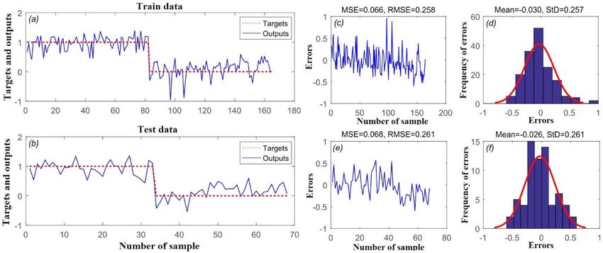
www.nature.com/scientificreports/
Figure 8. Flood inundation zone maps for the city of Amol produced by: (a) the SVR model, (b) the Wavelet-
SVR-Bat model, and (c) the Wavelet-SVR-GWO model. These maps were generated using ArcGIS Desktop
10.7.1, https://desktop.arcgis.com/en/.
Scientific Reports | (2020) 10:12937 | https://doi.org/10.1038/s41598-020-69703-7 9
Vol.:(0123456789)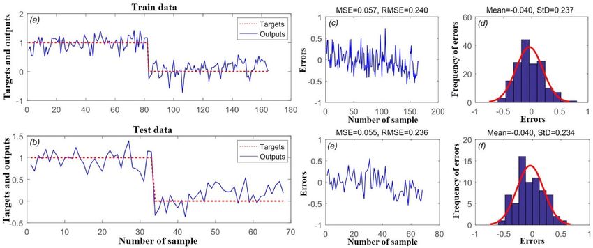
www.nature.com/scientificreports/

                                      Figure 9.  Pairwise agreement plots (PAP) showing results of pair-wise comparisons between: (a) SVR and
                                      Wavelet-SVR-Bat, (b) SVR and Wavelet-SVR-GWO, and (c) Wavelet-SVR-Bat and Wavelet-SVR-GWO.

                                                               Relative decrease in AUC (%)
                                       Excluded factor         SVR          Wavelet-SVR-Bat   Wavelet-SVR-GWO
                                       Distance from channel   38.4 ± 3.6   39.5 ± 4.2        39.1 ± 3.9
                                       Distance from river      31 ± 2.5    32.3 ± 3.1        33.1 ± 3.2
                                       Curve number            26.2 ± 3.4   25.9 ± 2.8        25.7 ± 2.4
                                       Slope                    8.7 ± 3.5    8.2 ± 2.6         8.4 ± 2.8
                                       Elevation                4.1 ± 1.9    4.6 ± 2.3         4.7 ± 2.9
                                       Precipitation            3.6 ± 0.5    3.5 ± 0.4         3.2 ± 0.6

                                      Table 4.  Overall importance of predictors in the three models used.

                                      some examples where several factors have led to flooding. However, there were significant differences in the
                                      contribution of flood conditioning factors to the modeling process (Table 4).

                                      Discussion
                                      Based on the different statistical evaluation metrics employed in this study, both hybrid models tested (Wavelet-
                                      SVR-GWO and Wavelet-SVR-Bat) showed superior performance to the standalone SVR model. The results also
                                      demonstrated that Wavelet-SVR-GWO produced more trustworthy flood susceptibility maps than the other

          Scientific Reports |   (2020) 10:12937 |                   https://doi.org/10.1038/s41598-020-69703-7                                     10

Vol:.(1234567890)
www.nature.com/scientificreports/
models. The GWO algorithm is flexible, robust, easy to enforce, and improves the performance of the model.
Mirjalili et al.33 investigated the optimization performance of GWO and found that it has considerable capacity
for optimizing models. Saxena and Shekhawat34 confirmed the satisfactory efficiency of GWO in optimizing
SVM for an air quality classification issue. Yang35 describes the characteristics of the Bat algorithm that lead
to its optimizing and improving model performance. Bat is a robust algorithm inspired by the echolocation
behavior of bats. Yang29 showed that it is able to outperform other metaheuristic algorithms, such as PSO and
genetic algorithm (GA), in terms of both convergence speed and improved local optima avoidance. In addition,
wavelet transformers are known to be strong decomposition tools that enable prediction models to access more
information at different dissected scales and dimensions of data domain36. Standalone models may not cope
with the non-stationary properties of data, either spatially or temporally, especially when dealing with highly
complicated spatial interrelationships and the problem of data scarcity (such as urban environments). Regard-
ing the benefits of Bat and GWO algorithms and wavelet transformers, the results of this study are in agreement
with previous findings34,37.
Information on the relative importance of flood conditioning factors (i.e., predictor variables) is of practical
relevance to natural disaster managers dealing with allocating and planning limited resources for flood hazard
management8. Kalantari et al.2 indicated that analysis of the relationship between flood events and geoenviron-
mental variables allows managers to focus on the influences of human activities. Although expert opinion-based
methods (e.g., analytical hierarchy process (AHP)) have been applied to analyze the relative importance of
geoenvironmental factors and determine their relationships with urban flood events, they are prone to subjective
judgments. In fact, expert opinion-based methods determine the weight of factors based on the pairwise compari-
son, which can be considered a drawback. Fernández and Lutz38 used the AHP method for urban flood hazard
zoning in Tucumán Province, Argentina, and concluded that, as flood-prone areas can be identified based on
expert opinions, this method can be a useful tool if flood event data and maps are not available. Machine learning
models use real flood occurrences to analyze the role of flood conditioning factors in modeling and determine
the contribution of variables39. This approach helps in reducing bias and subjectivity in decision-making11.
Importantly, as discussed by Khosravi et al.27, the relative importance of predictor variables to a model is probably
affected by the modeling strategy (i.e., model structure, etc.). Therefore, the relative importance of factors should
be investigated using at least two models. In our study, the relative importance of flood conditioning factors was
analyzed based on all three models (standalone SVR, Wavelet-SVR-Bat, and Wavelet-SVR-GWO), which showed
excellent performance. All models demonstrated that distance from channel made the highest contribution to
urban flood modeling, followed by distance from river, and curve number. This confirms results reported by
Darabi et al.4 and Falah et al.23, who investigated the importance of flood conditioning factors in urban areas.
The urban channel network generally has low conveyance capacity, resulting in flooding and inundation events
in urban areas. Rivers in the study area also have low conveyance capacity, and floods often exceed the flow
capacity, so inundation occurs frequently. However, there are limitations to increasing the capacity of existing
drainage channels, because of land availability in urban areas and u rbanization23. In other words, urbanization
in river/channel zones is the main cause of reduced drainage capacity, changes in hydrological and hydraulic
processes, and flooding in urban areas10. In addition, curve number, one of the main flood conditioning factors
in this study, is influenced by human activities (e.g., land-use change in urban areas or in upstream watersheds)
carried out to meet various needs such as residential, agricultural, industrial, mining, and other infrastructural
facilities. These pose major challenges to the sustainable growth of an area.
Concluding remarks
Flooding poses great threats to communities and property, especially in densely-populated urban environments,
where intensifying urbanization leads to severe floods by increasing the area of impermeable surfaces. Since
hydrometric stations are not available in urban areas, data scarcity is the main problem in spatial modeling of
flood susceptibility. This study presents two new hybridized models, wavelet-SVR-GWO and wavelet-SVR-Bat,
based on historical urban flood inundation events and using metaheuristic algorithms and wavelet transforma-
tion analysis. In a case study, Wavelet-SVR-GWO showed better predictive performance (AUC = 0.981, A = 0.926,
RMSE = 0.236) in flood susceptibility mapping for Amol city, Iran, than Wavelet-SVR-Bat (AUC = 0.972,
A = 0.882, RMSE = 0.261). Both hybridized models showed better performance than a standalone SVR. Thus
metaheuristic optimization algorithms (i.e., Bat and GWO) and wavelet transform analysis can considerably
enhance the learning and predictive performance of the standalone SVR model. The coupled wavelet-optimi-
zation algorithms could be a perfect fit for data mining models to find the best solution in a high-dimensional
complex problem space. In Amol city, high and very high flood susceptibility classes covered about 43% of
the study area and two schools fell into these areas. Using the robust flood susceptibility maps provided by the
hybridized models could improve the capability of urban systems in high and very high susceptibility classes to
evacuate floodwaters and reduce negative consequences for the inhabitants, both in terms of threat to human
health and damage to property. However, the hybridized models should be further tested in other urban areas to
validate their performance. Additional optimization algorithms, such as GA and PSO, should also be compared
with those used in the present study.
Methodology
The methodological workflow developed in this study comprised the following steps (Fig. 10): preparation of
dependent and independent variables, running the standalone SVR model, development of the two hybridized
models (Wavelet-SVR-BAT and Wavelet-SVR-GWO), model validation, and comparison of model performance.
Scientific Reports | (2020) 10:12937 | https://doi.org/10.1038/s41598-020-69703-7 11
Vol.:(0123456789)www.nature.com/scientificreports/
Figure 10. Flowchart of the methodology used in this study.
Urban flood inventory. Historical flood inundation events in urban environments provide vital informa-
tion for modeling. In this study, a total of 118 flood inundation locations were recorded by field investigations
and available reports in the Amol Municipality (see Fig. 1). A ratio of 70:30 was used to randomly split the flood
inventory dataset into two groups, for training (n = 83) and validation (n = 35) of the models.
Factors influencing urban flood inundation. There are no universal guidelines for selecting factors
that affect urban flood susceptibility, and previous researchers have considered different factors, depending on
the model used and data availability. In this study, the selection of the flood conditioning factors was based on
previous work by Darabi et al.11 and Falah et al.23 and data availability in the study region. The factors selected
to map urban flood susceptibility in this study were elevation, slope percent, distance from river, distance from
channel, curve number (CN), and precipitation (Fig. 11). River network was derived from an elevation layer
map with 5-m spatial resolution provided by the Amol city authority. The elevation of Amol city ranges between
59 and 137 m (Fig. 11a). Slope as a topographical factor influences water flow characteristics such as velocity
and discharge. It also impacts erosion and sedimentation processes. Lower slopes are generally seen in lowland
areas of a watershed, which makes these susceptible to flooding40. Hence, slope could be an important factor in
flood susceptibility investigations. Slope percent in Amol city varies from 0 to 25 (Fig. 11b). Rivers and channels
are main paths of water flow in cities, where rivers are a natural feature, and channels are human-made. Major
floods usually occur from rivers, but the inappropriate design of channels network can cause considerable flood-
ing. Therefore, this study considered distance from rivers and channels and calculated these layers by Euclidean
distance function. Distance from river in the Amol city ranges between 0 and 2,322 m (Fig. 11c), and distance
from channel varies between 0 and 1,499 m (Fig. 11d). Curve number is an important variable that influences
the permeability of soil or ground surface. This factor represents the impact of land use and soil permeability
features. To create the CN layer, an ArcCN-runoff function was implemented. There is a wide range of CN
in Amol city (40–100), which is high and shows a significant variation (Fig. 11e). Precipitation is the main
source of water flow, especially for flooding. To take its impact into account, we acquired the precipitation map
from the Mazandaran’s Forest, Range, and Watershed Management Organization. According to their report, 20
rain gauging stations were used for generating the precipitation map, based on the Kriging method due mainly
to lower RMSE value compared with other interpolation methods such as inverse distance weighting (IDW).
However, precipitation in the study area does not change dramatically, with a small spatial variation (672 to
684 mm year−1) in the study area (Fig. 11f). Further, the variance inflation factor (VIF) was calculated to investi-
gate the multicollinearity between the factors and avoid bias in the results. A VIF value higher than 5 indicates a
strong correlation between the factors and, accordingly, critical multicollinearity. Tolerance index, the reciprocal
of VIF, was also used, with values lower than 0.2, indicating critical multicollinearity.
Application of models. Support Vector Regression Algorithm. To solve regression issues and perform
short-term forecasting, the support vector regression (SVR) algorithm, which is a supervised learning tech-
Scientific Reports | (2020) 10:12937 | https://doi.org/10.1038/s41598-020-69703-7 12
Vol:.(1234567890)www.nature.com/scientificreports/
Figure 11. (a–f) Factors used to map flood conditioning in Amol city, and location of sites affected by previous
floods and used for both training and validation of the models. These maps were generated using ArcGIS
Desktop 10.7.1, https://desktop.arcgis.com/en/.
nique, can be applied41. The SVR algorithm, which is based on statistical learning theory, was first proposed by
apnik42. This method can be employed to look for relationships between input and output data, based on struc-
V
tural risk minimization. In contrast, Neural Network Algorithms (NNA) and conventional statistical methods
Scientific Reports | (2020) 10:12937 | https://doi.org/10.1038/s41598-020-69703-7 13
Vol.:(0123456789)www.nature.com/scientificreports/
are based on empirical risk minimization. Thus the SVR method has superiority in reducing the generalization
error as opposed to the learning error43. The purpose of SVR is to produce a function which explains the rela-
tionship between input and output data:
f (x) = w T ψ(x) + b (1)
where x ∈ Rn denotes input data vector, w ∈ Rn represents weight vector, b ∈ R is a deviation, and ψ(x) is a non-
linear mapping function that transforms input data into high-dimensional feature space. Parameters w and b are
based on the principle of structural risk minimization and are calculated as:
l
� �
1 2
�
∗
Minimize: �w� + C ξi + ξi
2
i=1
t (2)
yi − w xi − b ≤ ε + ξi
T
S.t. −yi + w xi + b ≤ ε + ξi ∗
ξi , ξi∗ ≥ 0
where yi ∈ Rn shows target data vector, C ≻ 0 is a penalty factor determining the tradeoff between training
error and model complexity, ξi , ξi∗ represents slack variables which adjust the upper and lower constraints on
the function f (x), and ε denotes the insensitive loss function, which represents the quality of a pproximation43.
Equation 2 can be solved utilizing Lagrangian formulation and its final solution:
n
f (x) = (αi − αi∗ )k(x, xi ) + b (3)
i=1
where αi , αi∗ are Lagrangian multipliers and k(xi , xj ) = �ψ(xi ), ψ(xj )� is the kernel function. Many different
types of kernel function can be included (e.g., polynomial, Gaussian radial basis, exponential radial basis).
It should be noted that the SVR technique is highly dependent on model and forecast error to define its
parameters, including penalty coefficient (C), permitted error range (ɛ), and kernel function parameters. For
instance, the training error will be quite high if C is at a very low level. On the contrary, if the penalty coefficient
is very high, the learning accuracy will improve, but the general adoptions of forecasting models will be low
in comparison with reality. When the number of supervised vectors is reduced on condition that ε is high, the
forecasting model is proportionately simple, but the accuracy will decline. On the other hand, if ε is rather low,
the complexity of the forecasting model increases, adoption decreases, and the accuracy of regression will be
enhanced. To find the optimized value of these parameters, in this study, the Bat and Grey Wolf evolutionary
optimization algorithms were applied44. A detailed description of the SVR algorithm can be found in Smola and
Schölkopf45.
Translation invariant wavelet kernel. Kernel functions have been used in many different pattern analysis and
ML techniques. These functions assist the SVR method in processing high-dimensional and infinite data, allow-
ing linear separability by mapping input space data to higher dimensions. In addition, kernel functions keep the
computational complexity of SVR reasonable in feature space46. Thus the number of support vectors and their
weights, but also the type of kernel functions, are important and affect the r esults47,48. A wavelet function can be
employed as the kernel function49. Generally, a wavelet function is defined as:
1 x−b
ψa,b (x) = √ ψ (a ≻ 0, b ∈ R) (4)
a a
where a and b represent dilation (scaling) and translation (shift) parameters, respectively, ψ(x) is the wavelet
base or mother wavelet, and indexed families of wavelets are obtained by changing a and b39,46. If a and b are
chosen on the basis of a power of 2 (a = 2j and b = k × 2j), the discrete wavelet transform (DWT) is as follows50:
1 x
ψj,k (x) = j ψ j − k
2 (5)
22
where k is a translation parameter and j is an integer representing the resolution level, i.e., the dilation parameter.
Based on the above, kernel function can be computed by inner products of wavelet function as:
N
′
x − bi′
xi − bi
k(X, X ′ ) = �ψ(X), ψ(X ′ )� = ψ ·ψ i a, bi , bi′ , xi , xi′ ∈ R (6)
a a
i=1
where X, X ′ ∈ RN are N-dimensional vectors and the translation-invariant wavelet kernel can be expressed a s51:
N
xi − xi′
k(X, X ′ ) = ψ (7)
a
i=1
It should be pointed out that there are various wavelet functions, such as Haar, Splines, Daubechies, Marr, and
Morlet. Gaussian function (Eq. 8) was used in this study due to its excellent reputation in terms of performance
Scientific Reports | (2020) 10:12937 | https://doi.org/10.1038/s41598-020-69703-7 14
Vol:.(1234567890)www.nature.com/scientificreports/
and possessing many useful features, as well as its strong learning capability52–54. Thus Eq. (7) was re-formulated
as:
2
−x
ψGaussian (x) = exp (8)
2
N
xi − x ′
2
i
′
k(X, X ) = exp − (9)
2a2
i=1
Finally, the general form of the wavelet SVR (WSVR) regression function can be written as:
� � 2
n N −
�
− x ′�
� � �xj j�
f (x) = (αi − αi∗ ) exp +b (10)
2a2
i=1 j=1
It should be noted that since WSVR has multidimensional analysis properties and high flexibility, and is a
generalization of the SVR algorithm, it can be employed to solve non-linear problems and approximation and
classification issues46. Studies have shown that the approximation effect of the wavelet kernel is far better than
that of the Gaussian k ernel52. Additionally, due to the redundancy and correlative features of the Gaussian kernel,
the training speed of the wavelet kernel SVM is rather fast in comparison with that of the Gaussian kernel S VM49.
More detailed explanations of wavelet SVR can be found in Zhang and H an49, and Su et al.55.
Bat Algorithm (BA). In 2010, Xing-She Yang established the Bat metaheuristic algorithm, which derives from
ats35. At night, bats can pinpoint their path and produce detailed images of
the echolocation characteristic of b
their prey by comparing the emitting pulse with its echoes. In the Bat algorithm, the position of each bat indi-
cates the potential solution and the quality of the solution is determined according to the best position of a bat
to its prey. The approach was developed based on the following three rules56:
1. All bats apply echo sounds to recognize the distance and distinguish the dissimilarity between food/ prey
and obstacles.
2. During the hunting period, bats fly unsystematically with certain velocity, at position Xi with fixed frequency,
fmin , and varying wavelength, , and loudness, A. Bats can also automatically adjust wavelength and rate of
pulse emission, r ∈ [0, 1], with regard to their distance to target.
3. Since loudness can vary in different directions, it can be assumed that the loudness changes from a maximum
(positive) to a minimum constant value.
Like other metaheuristic algorithms, there is a well-suited tradeoff between the two main features, intensi-
fication (exploitation) and diversification (exploration), which guarantee that the Bat algorithm (BA) can assist
in finding overall solutions57. According to the BA-SVR method, bats move within the parameter space and try
to detect some optimized parameters. In other words, defining the optimal value for the SVR parameters is the
main objective of implementing this a pproach37. For information, see A
li58, Sambariya et al.59, Yang35, and Yang
and Gandomi60.
Grey wolf optimization (GWO) algorithm. The Grey Wolf Optimization (GWO) algorithm can be employed
as another method to set optimum values of SVR parameters. The GWO algorithm was introduced by Mirjalili
et al.33 as a new metaheuristic method. This technique is a bio-inspired global optimization algorithm and, like
other metaheuristic methods, belongs to swarm intelligence approaches. The GWO algorithm is based on the
leadership hierarchy and the social behavior of grey wolves at the time of hunting. Wolves are social animals
that live in packs, and they have a hierarchy in their group. The leader of each pack, the alpha wolf ( α), dictates
decisions about hunting, sleeping, and walking time, and all the other group members must follow its orders.
However, despite the dominant manner of alpha wolves, democratic behavior can also be seen in the group.
In terms of hierarchy, the other wolves fall into three levels, called beta (β), delta (δ), and omega (ω ). The beta
wolves at the second level assist the alpha in making decision. They are the best candidates for alpha replacement
in due course. The delta wolves are in charge of defending the boundaries, warning the pack about any danger or
threats to its territory, and ensuring the safety of the group. At the time of hunting or sourcing food, deltas help
alpha and betas. The omega wolves have the lowest rank and rights in the group. They are not allowed to eat until
all other wolves have finished eating, do not play any role in decision making, and in fact have a victim role33.
However, in reality, theses wolves are a crucial part of the group, and their elimination can lead to fighting and
serious social problems for the overall group61.
In addition to the social hierarchy of grey wolves, another remarkable characteristic is their group hunting,
which can be summarized in three phases: (i) Tracking, chasing, and approaching prey, (ii) running after prey,
surrounding, and harassing the prey up to the moment it stops running, and (iii) attacking and k illing62,63.
In the GWO algorithm, mathematical modeling of wolves’ dominant social hierarchy behavior is performed
by generating a random set of solutions, of which the solution with the best fit is considered the alpha ( α). The
next best solutions are called beta (β ) and delta (δ), respectively, and remaining candidate solutions are called
omega. The hunting process (optimization) is led by α, β , and δ wolves, and ω wolves have to comply with these
Scientific Reports | (2020) 10:12937 | https://doi.org/10.1038/s41598-020-69703-7 15
Vol.:(0123456789)www.nature.com/scientificreports/
Predicted
Observed Non-flooded (absence) Flooded (presence)
Non-flooded (absence) True negative (TN) False positive (FP), Error type I
Flooded (presence) False negative (FN), Error type II True positive (TP)
Table 5. Contingency table used for evaluating models.
three groups. The following four stages are performed: encircling, trapping and surrounding the prey, detecting
prey location, attacking prey, and killing the prey (exploitation)5.
It is worth mentioning that GWO, as an optimization algorithm, has better search ability and higher accuracy
than Genetic Algorithm (GA) and Particle Swarm Optimization (PSO)33. The GWO algorithm can be employed
to find solutions to non-convex optimization problems. Its main advantages are its simplicity, ability to solve
real-world optimization problems, and fewer control parameters13. Supplementary information can be found in
Sulaiman et al.64, Niu et al.65, Jayakumar et al.66, Saxena et al.34, and Luo51.
Accuracy assessment. In the present study, the prediction performance of the models was assessed by
analyzing the agreement between observed data (flood inventory) and model results in terms of both presences
(i.e., flooded locations) and absence (i.e., non-flooded locations)11. Three different evaluation approaches were
used for assessing the accuracy of models in both the training (goodness-of-fit) and the validation (predictive
performance) steps. These were cutoff-independent metrics (Sensitivity, Specificity, Accuracy, Matthews Corre-
lation Coefficient, F-score, Misclassification Rate), cutoff-independent metrics (receiver operating characteristic
(ROC) curve), and root mean square error (RMSE).
Cutoff‑dependent metrics. All cutoff-dependent metrics were calculated based on a confusion matrix (also
known as the contingency table). The components of the contingency table are true negative (TN), true positive
(TP), false negative (FN), and false positive (FP) (Table 5), where FP and FN are the numbers of pixels errone-
ously classified (also known as error types I and II) and TN and TP are the numbers of pixels correctly classified.
Note that a probability holdout value of 0.5 was chosen since the presence and absence locations were equally
balanced, which is in accordance with Frattini et al.67 and Camilo et al.68.
True positive rate. True positive rate (TPR) (also termed sensitivity) is one of the most common evaluation
metrics and can be calculated as:
TP
TPR = (11)
TP + FN
False positive rate. False positive rate (FPR) (also known as 1 − specificity) can be calculated as:
FP
FPR = (12)
FP + TN
However, it should be noted that TPR and FPR are insufficient performance metrics, because they ignore false
positives (here the number of pixels erroneously identified as flooded) and false negatives (here the number of
pixels erroneously identified as non-flooded). In fact, they are useful only when used together.
Accuracy. Accuracy (A, also known as efficiency) is another common metric for evaluating model accuracy.
Accuracy determines the percentage of actual flooded points that are correctly classified by the model as:
TP + TN
A= (13)
TP + TN + FP + FN
Matthews correlation coefficient. The Matthews Correlation Coefficient (MCC) metric assesses the perfor-
mance of models based on the correlation rate between observed and predicted data69. MCC ranges from − 1 to
1, where − 1 indicates considerable disagreement between observed and predicted data and 1 indicates perfect
agreement. MCC is calculated as:
TP × TN − FP × FN
MCC = (14)
[(TP + FP) × (FN + TN) × (FP + TN) × (TP + FN)](1/2)
F‑score. The F-score (also called the F1 score or F measure) is calculated as:
2TP
F-score = (15)
2TP + FP + FN
Scientific Reports | (2020) 10:12937 | https://doi.org/10.1038/s41598-020-69703-7 16
Vol:.(1234567890)www.nature.com/scientificreports/
It can also be obtained based on the TPR and another evaluation metric, Positive Predictive Value (PPV), as:
PPV × TPR
F−score = 2 (16)
PPV + TPR
where PPV is TP/(TP + FP).
Misclassification rate, MR. Misclassification rate considers both the false positive and false negative compo-
nents and therefore reflects an overall error rate. MR can be computed as:
FP + FN
MR = (17)
FP + FN + TP + TN
Cutoff‑independent metric. The area under the ROC curve (AUC) is the most important evaluation metric in
natural hazard a ssessment40. The ROC curve simply plots the TPR (i.e., sensitivity) on the Y-axis against the FPR
(i.e., 1 − specificity) on the X-axis. It is considered the real measure of model evaluation because it simultaneously
includes all components of the confusion matrix and equitably estimates the overall quality of a m odel67. AUC
is bounded by [0, 1]: the larger the AUC value, the better the performance of the model over the whole range
of possible cutoffs. Based on the analytical expression for the ROC curve, denoted f, AUC can be calculated as:
1 1
AUC = f (FPR)dFPR = 1 − f −1 (TPR)d TPR (18)
0 0
Root mean square error. Root Mean Square Error (RMSE) is a frequently used measure of the agreement
between observed and predicted values. In the present study, the RMSE was used to evaluate all models. It can
be calculated as:
N
1/2
1
RMSE = (Si − Oi ) (19)
N
i=1
where Si and Oi are observed and predicted values, respectively.
Contribution of conditioning factors. The contribution of the flood conditioning factors (i.e., predic-
tor variables) to the modeling process (relative importance) was investigated using a map-removal sensitivity
analysis. The relative decrease (RD) in AUC values, which reflects the dependency of the model output on the
conditioning factors, was calculated. RD can be calculated using the following equation:
AUCall − AUCi
RD = × 100 (20)
AUCall
where AUCall and AUCi are the AUC values obtained from the flood susceptibility prediction using all condition-
ing factors and the prediction when the ith conditioning factor was excluded, respectively.
Received: 12 September 2019; Accepted: 24 June 2020
References
1. Dewan, T. H. Societal impacts and vulnerability to floods in Bangladesh and Nepal. Weather Clim. Extremes 7, 36–42 (2015).
2. Kalantari, Z. et al. Assessing flood probability for transportation infrastructure based on catchment characteristics, sediment
connectivity and remotely sensed soil moisture. Sci. Total Environ. 661, 393–406 (2019).
3. Khosravi, K. et al. A comparative assessment of decision trees algorithms for flash flood susceptibility modeling at Haraz watershed,
northern Iran. Sci. Total Environ. 627, 744–755 (2018).
4. Dewan, A. Floods in a Megacity: Geospatial Techniques in Assessing Hazards, Risk and Vulnerability 119–156 (Springer, Dordrecht,
2013).
5. Guha, D., Roy, P. K. & Banerjee, S. Load frequency control of large scale power system using quasi-oppositional grey wolf optimiza-
tion algorithm. Eng. Sci. Technol. 19, 1693–1713 (2016).
6. Auerbach, L. W. et al. Flood risk of natural and embanked landscapes on the Ganges-Brahmaputra tidal delta plain. Nat. Clim.
Change 5(2), 153–157 (2015).
7. Below, R., Wallemacq, P. Natural disasters. CRED—Centre for Research on the Epidemiology of Disasters (2018). https://www.cred.
be/annual-disaster-statistical-review-2017 (2017)
8. Bui, D. T. et al. Novel hybrid evolutionary algorithms for spatial prediction of floods. Sci. Rep. 8, 15364 (2018).
9. Alderman, K., Turner, L. R. & Tong, S. Floods and human health: a systematic review. Environ. Int. 47, 37–47 (2012).
10. Fernández, D. S. & Lutz, M. A. Urban flood hazard zoning in Tucumán Province, Argentina, using GIS and multicriteria decision
analysis. Eng. Geol. 111(1–4), 90–98 (2010).
11. Darabi, H. et al. Urban flood risk mapping using the GARP and QUEST models: a comparative study of machine learning tech-
niques. J. Hydrol. 569, 142–154 (2019).
12. Kalantari, Z. et al. Meeting sustainable development challenges in growing cities: coupled social-ecological systems modeling of
land use and water changes. J. Environ. Manag. 245, 471–480 (2019).
13. Liao, K.-H., Le, T. A. & Van Nguyen, K. Urban design principles for flood resilience: Learning from the ecological wisdom of living
with floods in the Vietnamese Mekong Delta. Landsc. Urban Plan. 155, 69–78 (2016).
Scientific Reports | (2020) 10:12937 | https://doi.org/10.1038/s41598-020-69703-7 17
Vol.:(0123456789)You can also read