Development of a wind turbine drive train engineering model
←
→
Page content transcription
If your browser does not render page correctly, please read the page content below
Development of a wind turbine drive
train engineering model

                         Abraham Derks,
                         August 12, 2008

                                           1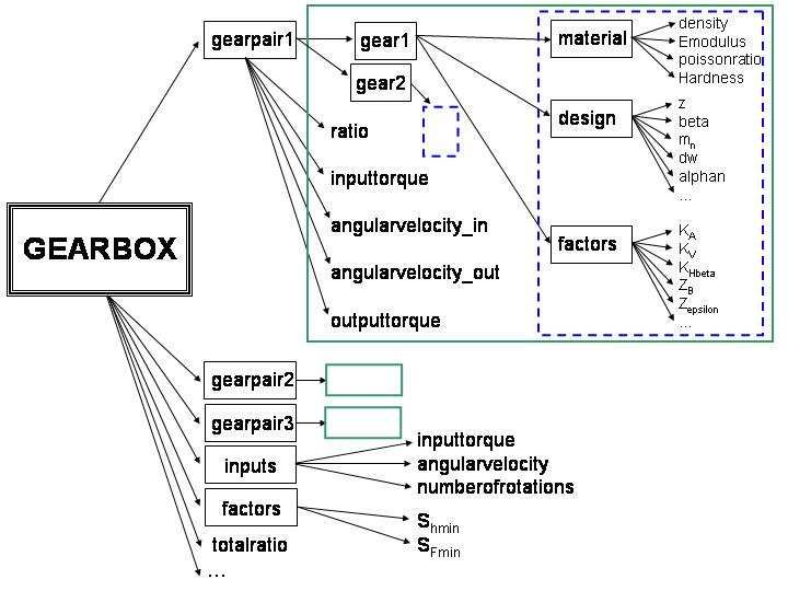
Preface

My interest in renewable energies started after I saw a documentary on visions on
the future of the energy economy. Both the many drawbacks of the dependence of
the world on fossil fuels and the predictions for the future were shown. The urgent
need for a change was explained in a way that I found truly inspiring [I1].
After courses on the various renewable energies, I found wind energy the most
interesting discipline because of its multidisciplinary nature and the matureness of
the industry. That being said, what probably interests me the most is the
combination of grace and sheer size… modern wind turbines are BIG ánd beautiful!

I wanted the aforementioned aspects to play a role in my choice for a graduation
project and succeeded after some good discussions with my later-to-be supervisor
Michiel Zaayer on the topic of design modelling and optimisation.
I found the topic of optimisation incredibly interesting as it models the philosophical
search for the one thing every engineer strives for without knowing exactly what it
is…’The best design’.

During the past year, an optimisation model of a wind turbine drive train was created
to investigate the effect of up scaling on the realization of an optimum design. This
report presents the results of this study, forming the final thesis as part of my
graduation at the faculty of Aerospace Engineering at the Delft University of
Technology.

I would like to thank Michiel Zaayer for his valuable feedback and encouragement
during this lengthy project. Furthermore, I would like to take the opportunity to
thank Giorgia for helping me so much and Martijn for letting me hijack his room and
computer for a year...I appreciate it !

Bram Derks,

August 12, 2008

2
3
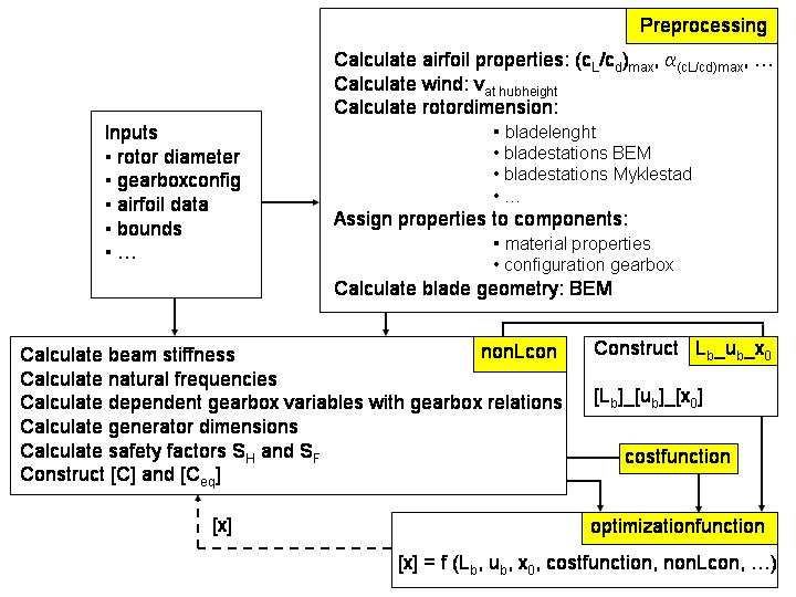
Table of Contents

1      INTRODUCTION .................................................................................................................................8
    1.1       DESIGN AND OPTIMIZATION RESEARCH OF WIND TURBINES..............................................................8
    1.2       THE RESEARCH OBJECTIVE .............................................................................................................10
    1.3       THE APPROACH...............................................................................................................................11
    1.4       OVERVIEW OF THE REPORT .............................................................................................................11
2      WIND TURBINE EVOLUTION .......................................................................................................13
    2.1       WIND ENERGY IN A HISTORICAL CONTEXT .....................................................................................13
    2.2       THE SHIFT FROM ONSHORE TO OFFSHORE; BIGGER = BETTER.........................................................16
    2.3       MODERN WIND TURBINE LAYOUT ...................................................................................................17
    2.4       THE WIND TURBINE IN THIS RESEARCH ...........................................................................................18
3      THE DESIGN PROCESS ...................................................................................................................19
    3.1       THE DESIGN PROCESS .....................................................................................................................19
    3.2       THE REAL-WORLD DESIGN PROCESS ...............................................................................................21
    3.3       THE NUMERICAL DESIGN PROCESS ..................................................................................................22
4      THE WIND TURBINE DRIVE TRAIN............................................................................................25
    4.1     DESCRIPTION OF THE DRIVE TRAIN .................................................................................................25
       4.1.1    General constraints for the drive train ..................................................................................25
    4.2     THE ROTOR .....................................................................................................................................26
       4.2.1    Function and layout of the rotor............................................................................................26
       4.2.2    Design variables and constraints for the rotor......................................................................26
       4.2.3    Aerodynamic design relations ...............................................................................................27
       4.2.4    Rotor constraint relations......................................................................................................31
       4.2.5    Limitations and general remarks on the gearbox model .......................................................35
    4.3     THE GEARBOX ................................................................................................................................36
       4.3.1    Function and layout of the gearbox.......................................................................................36
       4.3.2    Design variables and constraints for the gearbox .................................................................39
       4.3.3    Gearbox constraints relations ...............................................................................................43
       4.3.4    Limitations and general on the gearbox model .....................................................................51
    4.4     GENERATOR ...................................................................................................................................53
       4.4.1    Function and layout of the generator ....................................................................................53
       4.4.2    Design Variables and constraints for the generator..............................................................53
       4.4.3    Limitations and general remarks on the generator model.....................................................54
    4.5     THE COST MODEL OF THE DRIVE TRAIN...........................................................................................54
       4.5.1    Limitations and general remarks on the cost model ..............................................................55
5      IMPLEMENTATION OF THE DESIGN MODEL .........................................................................56
    5.1       MATLAB .........................................................................................................................................56
    5.2       STRUCTURE AND LAYOUT...............................................................................................................57
6      RESULTS AND DISCUSSION ..........................................................................................................62
    6.1       RESULTS AND DISCUSSION OF THE MODEL......................................................................................62
    6.2       RESULTS AND DISCUSSION OF THE IMPLEMENTATION.....................................................................64
7      CONCLUSIONS..................................................................................................................................68
8      THE RECOMMENDATIONS ...........................................................................................................69

4
List of figures
FIGURE 1: DESIGN CONSIDERATIONS FOR A WIND ENERGY CONVERSION SYSTEM, REPRODUCED FROM [B6]....9
FIGURE 2: GROWTH IN SIZE OF COMMERCIAL WIND TURBINES, REPRODUCED FROM [B2] ..............................17
FIGURE 3: CUT AWAY VIEW OF A WIND TURBINE NACELLE, REPRODUCED FROM [B5]....................................25
FIGURE 4: BLADE ELEMENT FORCES, REPRODUCED FROM [MI1] ....................................................................28
FIGURE 5: 61.5 METER WIND TURBINE BLADE, REPRODUCED FROM [B8]........................................................30
FIGURE 6; D-SHAPED BEAM ELEMENT, REPRODUCED FROM [B11] .................................................................31
FIGURE 7: HELICAL GEAR ...............................................................................................................................37
FIGURE 8: SPUR GEAR ....................................................................................................................................37
FIGURE 9: GEAR NOMENCLATURE, REPRODUCED FROM [I12] .........................................................................38
FIGURE 10: PARALLEL GEAR SYSTEM,............................................................................................................39
FIGURE 11: EPICYCLIC GEAR SYSTEM,............................................................................................................39
FIGURE 12: THE STRESSES IN CONTACTING GEAR TEETH, REPRODUCED FROM [I13].......................................43
FIGURE 13: GENERATOR DIMENSIONS, REPRODUCED FROM [P3]....................................................................53
FIGURE 14: STRUCTURE OF THE PROGRAM. ....................................................................................................59
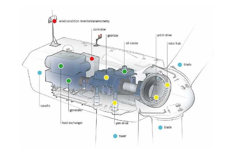
FIGURE 15: STRUCT 'GEARBOX'. .....................................................................................................................60
5
List of tables
TABLE 1: EXAMPLE RESULTS ..........................................................................................................................23
TABLE 2: K-FACTORS FOR THE CALCULATION OF THE DYNAMIC FACTOR.......................................................48
TABLE 3: PHASES AND PARTS OF THE PROGRAM .............................................................................................58
TABLE 4: VERIFICATION OF 'BLADEGEOMETRY_CALCULATION. LAMBDA = 6; B = 3......................................63
TABLE 5: VERIFICATION OF 'MYKLESTAD_FLAPWISE'....................................................................................64
TABLE 6: INPUT VALUES AND RESULTS FOR GEARBOX ...................................................................................66
TABLE 7: VERIFICATION OF 'BLADEGEOMETRY_CALCULATION'. LAMBDA = 1; B=12 ....................................75
TABLE 8: VERIFICATION OF 'BLADEGEOMETRY_CALCULATION. LAMBDA = 10; B = 2 ...................................76

6
Abstract

Wind turbines grow bigger every day. With rotor diameters exceeding the size of a
soccer pitch [I1][I3], it s not hard to imagine that designing such gigantic structures
is a formidable task. The multidisciplinary nature of wind turbine design adds to the
complexity of this task, as the subsystems of a wind turbine need to be tuned with
respect to a common objective to achieve a cost effective and structurally sound
design.

This rapport describes the construction of a model that can be used in an
optimization routine with the goals to automatically design an optimized wind turbine
drive train on the conceptual level and to allow the investigation of changes in
subsystem design with increasing rotor diameter. A secondary objective is to gain
insight in the construction of an optimization model of a wind turbine drive train and
the problems one encounters during implementation.

The drive train under consideration consists of three subsystems: the rotor, the
gearbox and the generator. Only the necessary level of detail to describe the
relationships between the subsystems and their geometry and constraints is
implemented.
Without making a trade off between computer languages, Matlab’s optimization
toolbox was used for the implementation.

The model and constraint of the rotor has been verified. The gearbox model has not
been verified due to lack of reliable data. The primary objective has not been met
due to the inability of the optimizer to find a global optimum. Also, the optimizer was
only able to deal with the implemention of the constraints and models if they were
further simplified.

                                                                                     7
1 Introduction 1.1 Design and optimization research of wind turbines Wind energy use has increased impressively over the last decades. Especially during the late 1990’s the developments were extremely fast and wind energy established itself as a main source of the world’s energy and a multibillion-Euro industry. The need for alternatives to the finite fossil fuels and the negative effects of these fuels for the environment, have driven the fast developments. Wind turbines have developed from relatively simple 50 kWatt turbines in the beginning of the 1980’s to complicated multi-Megawatt turbines that generate enough electrical energy to power a complete city. With the increasing size, also the complexity of designing a wind turbine increased. Designing wind turbines that are cost-effective is a challenge because they have to compete with conventional power systems on the basis of cost price per kilowatt- hour. The cost of conventional energy is mainly made up of the price of the fuel being used, while the cost of (offshore) wind turbines is mainly made up of operation and maintenance cost (O&M), installation cost and capital cost. Although fuel prices have risen sharply, especially during the last few years, there is still an imbalance between prices for conventional energy and those for energy from the wind. This means that in order to improve competitiveness of wind turbines, there must be a reduction in both maintenance and capital cost. 8
Figure 1: design considerations for a wind energy conversion system, reproduced from [B6].

Three of the main technological advancements that would cut these costs are found
to be [B1]:

    -   Scaling-up wind turbine size for low capital cost per kilowatt(-hour).
    -   Integrated design aiming at, for example, reduction of mass to cut installation
        cost.
    -   More efficient energy conversion

These three technological challenges are strongly interrelated. They all have to be
met in order to truly improve wind turbine competitiveness. More efficient conversion
and weight reduction are only possible if the subsystems of the wind turbine are
integrated in a way that improves the performance of the wind turbine as a whole.
Not so much the performance of the subsystem in itself is important, but the
performance of the total system. This means that the subsystems of a wind turbine
should be optimized with respect to the operation of the total wind turbine in mind.
Such optimization is difficult to achieve in practice because a wind turbine design
involves aspects that originate from many areas of engineering, and the interactions
between the different disciplines need to be exploited optimally. See Figure 1 for the
main considerations in wind turbine design. It gets even more complicated when
taking into account up scaling of wind turbines because all subsystems within the
turbine get bigger, heavier, and outside the scope of current design.

                                                                                             9
1.2 The research objective It is an interesting question how the designs of the subsystems in a wind turbine are interrelated. To investigate this in relation to the mentioned up scaling, the following research objective was formulated. “Construct a design model and investigate the effect of up scaling on the optimum design of an offshore wind turbine“ Designing an optimised system requires iterations. A current design is analysed and points of improvement are identified. The design is altered and analysed again to see if the performance of the design has improved. Then again points of improvement are identified, altered and analysed. This process continues until the design is considered optimal. The general procedure consists of identification of points of improvement, alteration of characteristics, generation of the new design and evaluation of this design. This process can be modelled by a computer, which can perform this cycle very quickly and very ‘smart’. Therefore the research is confined to using a computer to build an optimization routine capable of optimizing the drive train of a wind turbine with respect to a to- be-defined objective. The drive train is chosen for reasons outlined in chapter 2. For this optimization, no trade off between programming languages is made; the language chosen for the implementation is Matlab. The reasons for this choice are that it is readily available, easy to work with and includes a specialized optimization toolbox. The drive train is considered a three-subsystem design consisting of the rotor, the gearbox and the generator. The philosophy is to take the simplest level of detail while still being able to define the geometry of the subsystems and to take into account some major constraints. Apart from setting up a working model to do research on design changes, a secondary objective is to gain knowledge and experience with the implementation of a design model for a wind turbine. 10
1.3     The approach

The main steps in the approach were identified as:

•   Definition of the objective

•   A literature research, including:

    -   Analysis of design processes
    -   Research on optimization modeling
    -   Demarcation of the system under consideration
    -   Analysis of subsystem design options
    -   For every subsystem an analysis of the parameters that influence the design
    -   Identification of the design variables
    -   Identification of the bound constraints
    -   Identification of the functional constraints

Subsequently;
•   Modeling the subsystems and constraints

•   Verification of models and constraints

•   Optimization research for different rotor diameters

•   Verification of results of the optimization research

Although the list gives a step-by-step view on the process, many steps were
intertwined. Especially during modeling, which was by far the most elaborate phase
of the project, a lot of research was still needed on how to model the subsystems. It
was undoable to identify all parameters beforehand because of the multidisciplinary
nature and the multitude of variables needed in the model.

1.4     Overview of the report

This report comprises 8 chapters. Chapter 2 gives an overview on the historical
developments and gives an introduction to modern wind turbines. It places the

                                                                                  11
evolution towards offshore placement of wind turbines in a historical context and explains the working principle of wind turbines. The design process as a general engineering practice is explained in chapter 3. It will be indicated that a mathematical procedure can mimic the steps taken in the design process. Chapter 4 zooms in on the wind turbine drive train. The models of the multiple subsystems are described and the constraints that have to be taken into account when designing these subsystems are discussed. It will be shown how these constraints can be accounted for. The objectives for the design of a drive train are identified in the last part of this chapter. The implementation in the computer is described in chapter 5. A short description of Matlab will be given and the structure of the written code will be explained, including the main steps that the program takes in its search for a ‘best’ design. Chapter 6 is reserved for the results and the discussion of these. Since the program has difficulties in finding a ‘best’ design, part of this chapter is devoted to finding a reason why this is the case. In the last part of this chapter, both the primary and the secondary objective will be evaluated. A summarization of the conclusions is given in chapter 7, some suggestions for future research are given in chapter 8 12
2       Wind turbine evolution

2.1      Wind energy in a historical context

The first use of wind energy is thought to have occurred as early as 900 A.D, when
windmills were used for grinding grain and pumping water [B1]. Around the 12th
century windmills emerged in Europe and around the 14th century became the main
source of energy. It’s hard to recognize the major impact windmills had on landscape
and society in The Netherlands. The rise of the Netherlands during the golden age is
partly due to the advancements in windmill engineering as they sped up the
machining of wood for building ships and gave the possibility to shape the landscape
and win the battle against the water.

The technology developments were mainly driven by inventive millers to improve the
efficiency of their mill and ease their heavy work. The fantail, invented around 1735,
enabled the windmill to yaw automatically.
As scientific methodology developed, a more systematic approach towards windmills
was adapted, where testing and evaluation of tests became standard. This led to the
discovery by Englishman John Smeaton of three basic rules still applicable today
[B1]:

    -   The speed of the blade tips is ideally proportional to the wind speed
    -   The maximum torque is proportional to the speed of the wind squared
    -   The maximum power is proportional to the speed of the wind cubed.

This knowledge led to more development in the field of wind engineering; in 1807 a
system was developed by Sir William Cubitt to automatically adjust the sail setting to
the wind speed and preventing the sails from being ripped apart in heavy winds, the
so-called patent sails.[I1]
Around the mid-19th century, windmill use gradually declined in Europe as the steam
engine eliminated the need for the (sometimes absent) wind. However, around this
time there was an increased interest in wind energy in the United States, where
windmills were used for pumping water in the deserted areas of the west. These
mills, with many blades and a simple regulating system could run unattended for
long times and needed little wind to be operational.

                                                                                   13
When electrical generators appeared around the end of the 19th century interest
developed to use windmills to power them. The term wind turbine came into use to
depict such a combined generator – windmill system.[I5]
Charles F. Brush erected the first wind turbine in 1888. Using the American concept
with 144 blades made of cedar wood and 17 meters rotor diameter he reached a
power rating of 12 kWatt, see picture 1
.
picture 1: The 12kW Brush wind generator, reproduced from [I5]
Around the 1930’s the use of small electrical generators started to decline as a result
of expansion of the central electrical grid. One significant wind turbine built around
the time was the Smith-Putnam machine, a huge 1.25 MWatt twin bladed wind
turbine with a rotor diameter of 53.3 meters, see picture 2. Starting operation on 19
October 1941, it was the largest turbine in the world until the 1980’s. Being so large,
the Smith-Putnam turbine suffered from problems in the bearings and blades. In
1943 it had to be taken out of service when a blade broke off. Although it had many
problems, the Smith-Putnam wind turbine helped to improve wind turbine technology
and showed the potential of using the wind to generate electricity in large quantities
[I6].
14picture 2: The Smith-Putnam wind turbine, reproduced from [I7]
Until the oil crisis of the 1970’s wind energy was basically abandoned. This changed
as fossil fuels became expensive and environmental concerns grew. Research and
subsidy programs were stimulated in countries that wanted to be less dependent on
oil. In California wind turbine exploitation began to make economic sense due to
regulatory changes, leading to the great California wind rush. Several designs were
developed and at the end of 1985, more than 1000 MWatt was installed in this state
alone. The market in the United States disappeared in 1986 with the abandonment of
Californian support schemes. During this wind rush, most wind turbines originated
from Denmark, where manufacturers built a strong track record with simple, solid
machines, which came to be known as the Danish concept. The emergence of Danish
manufacturers can be considered the start of a professional wind turbine industry.
152.2 The shift from onshore to offshore; Bigger is Better
Three important rules were mentioned in paragraph 2.1 regarding the influence of
wind speed on maximum torque and maximum power. Another important
observation is the increase in available power with swept area of the rotor and wind
speed. The actual power produced by a wind turbine is:
1
Pmax = η C p ρV03 A (2.1)
2
In this equation, η is the mechanical (including electrical) efficiency, C p is the
powercoefficient, which represents the ratio of power available in the flow and the
power extracted from the flow. ρ is the density of the flow, V0 the undisturbed
speed of the flow, and A the rotor area.
Looking at equation (2.1) it is obvious that the wind speed has a profound effect on
the power produced by a wind turbine. Of course, this is the reason why it makes
sense to place wind turbines at windy locations. Although not as large, a good
aerodynamic design (for a high value of C p ) and a large swept area also have an
important positive influence on the actual power production.
The importance of good wind resource, large rotor swept area and the scarcity of
suitable locations because of social opposition for onshore installation (the classical
NIMBY complex see [I8]), led wind turbine manufacturers offshore during the late
1990’s. The wind resources are generally better at sea and large rotor diameters are
not much of a problem if placed far enough from shore as to not influence the
landscape. However, putting wind turbines offshore also means increasing piecewise
cost for grid connection and O&M. This is main reason why wind turbines grew
massively over the last decade (as depicted in Figure 2) and are expected to grow
even larger in the future; It’s more cost effective to put fewer but larger wind
turbines offshore than building many small wind turbines with the same total swept
area at those remote locations.
16Figure 2: Growth in size of commercial wind turbines, reproduced from [B2]
2.3 Modern wind turbine layout
As mentioned in paragraph 2.1, many Danish wind turbines were installed in the
1980’s. The Danish concept was developed, which is a horizontal axis, stall
regulated, fixed speed wind turbine (HAWT), with a three-bladed upwind rotor and
the asynchronous generator coupled directly to the grid. Since its rise, the Danish
concept has been somewhat of a standard against which other turbines are judged.
They were a starting point for developments towards the newer generation of wind
turbines, which are mostly three bladed and of the variable speed, pitch regulated
type. The basic subsystems of a typical horizontal axis wind turbine remained the
same, these include:
- The rotor, including blades and hub
- The drive train, including the gearbox and the generator
- The nacelle, including the housing and yawing system
- The tower
- The foundation
- The control system
- The electrical system, including cables, transformers and power electronics.
17The energy conversion occurs in the rotor drive train combination. The kinetic energy of the flow is converted into electrical energy in the generator. Because the electrical energy must be transported to the net, transformers and power electronics are needed to deliver the energy in a suitable form. The other subsystems are either supportive or ancillary. The supportive subsystems carry the rotor drive train combination and include the nacelle, the tower and the foundation. The ancillary subsystems include the control and yaw system, which guide the rotor drive train combination to adapt to changing conditions in the environment and keep it at its optimum operating point. The terminology of subsystems is always bit tricky as it is often not very clear where one subsystem ends and another starts. Different manufacturers use different terms for the same subsystem or subsystem. Of course this is just a matter of definition. Although not correct according to the above terminology, in the remaining of this research the rotor is considered part of the drive train. 2.4 The wind turbine in this research The foregoing discussion made clear that offshore use of wind turbines resulted in a rapid growth of rotor diameter. This is the rationale behind directing the research towards subsystems design of a wind turbine in relation to changing rotor diameter. Furthermore, the drive train can be considered the ‘heart’ of the turbine because this is where the energy conversion takes place. The research will therefore be confined to investigating the effect of a change in rotor diameter on the design of the rest of the drive train: the gearbox and the generator. 18
3        The Design Process

3.1      The design process

The Longman dictionary of contemporary English defines design “the arrangement of
parts that go into human production” [B4].

From a conceptual point of view, a design is a combination of values for the
quantifiable parameters involved in the problem. A subset of the quantifiable
parameters is formed by the design variables; Those are the quantities that lie under
the control of the designer and with which he directly influences the purposefulness
of the final combination of parameters. Of course, there are also parameters that are
outside the control of the designer. Choosing which of the variables are taken as
independent often requires an evaluation of the constraints and the objective the
designer has to deal with.

To illustrate the concept of design, the following problem is considered;
During the design of a wind turbine it is interesting to investigate what the optimum
design of a wind turbine would have to be with regards to costs. After some
research, a manufacturer found that the cost of its turbines is a function of three
design variables: The height of the hub of the turbine    H , the diameter of the rotor
D and the power delivered P . He expects that:

         g * H + h * D 2.4
Cost =                     (3.1)
              i * P2

where    g , h and i are scaling factors, that can originate from a range of causes,
such as the production process, the logistics, the expected revenue per Kilowatt,
etc. The objective would be to design a system, in this case a combination of design
variables H, D and P, for which the cost are minimized.

The constraints limit the allowed values for the variables. The constraints can
originate from (scientific) research, limitations in resources, or assumed as being
valid and can be either set (also called box or bound) contraints or functional

                                                                                    19
constraints. A set constraints is constraint on the value of a design variable, in the
example above there could be several set constraints.
For example, a set constraint could be that the towerheight must be larger than a
meters, but cannot be larger than b meters, because of limitations in the production
facilities: a < H < b (3.2)
An additional set constraint could be that the blades should not be smaller than 0.5c,
but also not longer than 0.5d, because of logistical considerations. The set
constraints on the rotor diameter are: c < D < d (3.3).
The maximum delivered power is not constrained in this case, but the power
delivered should not be smaller than or equal to zero, because it would mean that
the manufacturer would have created an enormous fan, which is not very usefull
offshore and probably would not generate a lot of revenue: P > 0 (3.4)
(Formally, this could be taken into account by changing the objective function and
making the cost very high for this situation, but this is not considered any further)
A functional constraint is a constraint on the value of a function of (multiple) design
variable(s). An example of such a constraint would be to model the power as a
product of a factor and the diameter: P = e * D 2 (3.5)
in which e is a factor which is determined by choices of the designer and includes
(amongst others) the C p -factor in (2.1). In this example, e is considered fixed.
The turbine under consideration is an offshore wind turbine, for which the hubheight
H must be at least equal to the sum of the length of the blade and a factor f
representing the maximum expected waveheight at the location. Thus, another
1
functional constraint is H ≥ * D + f . (3.6)
2
The design space is the imaginary space made up of all possible combinations of the
design variables H , D , P . Every point in this design space has a corresponding
value for the objective function. The constraints are imposed on the design space,
thereby creating the feasible region. In this case, we have 3 designvariables and the
design space is a 3-dimensional space with every axis representing a design variable
that can be chosen within the feasible region, determined by its bound and/or
functional constraints. As a result of equation (3.5) the feasible region is a curved
20sheet. The design process is the method to find the optimum set of design variables
with respect to the objective while never violating the constraints.
3.2 The real-world design Process
The design process in a commercial organization is an iterative (decision making)
process that has an alternating divergent-convergent character. It starts with the
‘Mission Need’ definition phase, in which the need is meticulously formulated. After
this, the requirements and functional analysis starts, with the goal to arrive at a
complete understanding of the problem to be solved for the end-user. Every function
that needs to be fulfilled by the end product to meet operational requirements must
be identified. Subsequently, technology studies are performed and candidate
concepts and architectures are generated. This is the divergent part of the design
process, in which as many ideas as possible are generated
After this, a process is started of working through all of the concepts far enough that
their feasibility can be judged. During the subsequent trade-off phase, the feasible
designs are weighed on the predetermined trade-off criteria, and the design process
converges towards one chosen concept
At this stage of the design process there is merely a worked-through concept, not a
final product design and the process starts to come to an end product. The described
process of generating concepts and doing trade-offs is repeated on subsystem and
component level throughout the next stage of the design process, which is
characterized by an increasing convergence towards the final product. Major design
decisions and the ones involved with long lead times should be made first. The later
a major design decision is made, the more costly it will be, because more and more
derived design decisions will have to be reviewed. Design changes are analyzed for
their effects on the fulfillment of the final objective (need) and the totality of system
requirements. For this reason, this part of the design process involves a lot of
interaction between different design groups to check that a design change does not
have a detrimental effect on the performance of the overall design, including the
performance of other disciplines. The inability to recognize that system requirements
can differ from disciplinary requirements is a general recurring problem in product
development.
213.3 The numerical design process The design process can be modelled as an optimization problem and can be numerically solved by an optimization algorithm. The derivative based search algorithms are widely used for this goal. This kind of algorithm starts at values X0 and searches through the feasible region by making sensitivity analysis of the bjective function with respect to the design variables. It checks the slope of the objective function in the direction of the different design variables, to see whether the value of the objective function would be increasing or decreasing in that particular direction. It then chooses the slope towards the lowest point. If the optimizer arrives at a point X for which the value of the objective function would only be increasing in either search direction, it recognizes this as a minimum. The similarities between the numerical optimization algorithm and the real world design process are that starting at a value, changes in the design variables are constantly checked for their influence on the objective and the best change is choosen to iterate towards an optimum solution. The Mathematical formulation The mathematical formulation, written in vectors, of the above problem is as follows: min Cost(X) subject to: A*X
a b
LB = c , UB = d .(3.8)
0 ∞
The power, as given in equation (3.5), is considered a nonlinear equality constraint
that can be written as:
e*D 2 − P = 0 (3.9)
This simple example is worked out with Matlab (see paragraph 5.1 for a description
of general method). As this is merely an example, the values for the constants
a,...., i are arbitrarily chosen as:
Constraints: Factors:
a = 0; g = 10;
b = 120; h = 1.5;
c = 10; i = 50;
d = 200;
e = 0.5;
f = 15;
The results for randomly chosen starting values for X0 are shown in Table 1.
H0 D0 P0 H D P Cost
101.062 31.324 23.049 119.916 200.000 20000.000 0.041728
108.623 36.284 17.203 119.797 200.000 20000.000 0.041727
89.333 22.137 6.459 116.671 200.000 20000.000 0.041725
82.790 33.905 1.280 24.781 19.562 191.331 1.942670
107.451 39.282 1.043 25.443 20.886 218.117 1.724428
80.912 26.254 14.649 119.792 200.000 20000.000 0.041727
83.818 20.259 22.812 116.352 200.000 20000.000 0.041725
90.623 43.413 14.100 119.848 200.000 20000.000 0.041728
93.097 21.476 2.489 115.000 200.000 20000.000 0.041723
82.733 37.821 8.233 77.816 48.889 1195.065 0.414707
Table 1: example results
23The actual values of this example are not so important since the values are arbitrarily chosen. What ís important are some trends that can be seen in this table. It is clear that the optimization mostly finds the same minimum value for Cost, irrespective of the starting values of the optimization. Sometimes, however, the optimization results in a value for Cost, which is clearly not a minimum, see calculations 4, 5 and 10. Looking at the starting values for those calculations and comparing them to the values for the other runs, there is no clear reason why the optimization results in a suboptimal value. This is a phenomenon that often occurs in numerical optimizations. The explanation for this is that the optimizer that was used is a gradient based search algorithm for which it cannot be guaranteed that an optimum is global [I10]. It could be the case that the optimizer recognized a local minimum only and does not recognise that there is a value elsewhere in the feasible region where the objective function attains a smaller value. 24
4          The Wind Turbine Drive train

4.1        Description of the drive train

As mentioned in paragraph 2.3, the drive train considered in this research consists of
the rotor, the gearbox and the generator. In Figure 3, a typical modern wind turbine
drive train is shown. As can be seen, many auxiliary systems are attached to the
drive train, such as coolers, but these systems are not taken into consideration in
this research. Only the three major subsystems will be modeled.

Figure 3: Cut away view of a wind turbine nacelle, reproduced from [B5].

4.1.1      General constraints for the drive train

The three subsystems that are being modeled are physically connected in a real-
world drive train. This implies that some physical quantities are being transferred.
This poses constraints on the input and output values of these quantities for the
subsystems. For the drive train the following general constraints are valid:

Ω rotor = ωin , gearbox

                                                                                   25
Trotor = Tin, gearbox
ωout , gearbox = ωin, generator
Tout , gearbox = Tin , generator
where T is the torque, Ω is the rotational velocity of the rotor, and ω is the
rotational velocity of the gearbox and generator.
4.2 The rotor
4.2.1 Function and layout of the rotor
The rotor under consideration consists of the hub and the blades. In a wind turbine,
more subsystems are included such as, for example, the pitch system, but these are
not modeled. Since the aerodynamics of the blade is responsible for its main
function, energy conversion, it is also the driving aspect for the design. Therefore,
the shape of the blades is determined with respect to aerodynamics only. In
contradiction to the rest of the drive train, the aerodynamic design of the blade, as
considered in this research, is not an optimization process such as explained in
chapter 3. The ideal shape of the blade can be computed directly whenever the
number of blades, the tip speed ratio and airfoils are chosen by the designer.
The structural part of the blade, however, must be optimized with the constraint that
that the rotor must be dynamically reliable.
4.2.2 Design variables and constraints for the rotor
The design variables of the rotor are originating from two disciplines; aerodynamics
and structural mechanics.
Aerodynamic design variables
The design variables for the aerodynamic design of the blades are:
- The tip speed ratio λ
- The number of blades B
- The rotor radius Rtip
These design variables are somewhat different then the other design variables, as
the designer chooses them, after which the optimization of rest of the drive train will
26start. Therefore, the design variables for the aerodynamic design are constrained to
the values chosen by the designer.
Structural design variables
The only design variable for the structural design of the blades is:
- The wall thickness δ of the D-shaped load-carrying element in the blade.
The bound constraints for the rotor:
λ = λinput
B = Binput
Rtip = Rinput (4.1)
δ min < δ < δ max
The functional constraints rotor.
During the optimization, a check has to be made on whether there is a safe margin
between the natural frequency and the 1p and 3p forcing frequencies. If the natural
frequencies of the blade tend to coincide with either of these, designing a stiffer
load-carrying element can increase the blade’s natural frequencies. In this research,
only flapwise vibration (out of the rotor plane) is taken into account.
- The first three natural frequencies of the blade should not coincide with the 1P
or 3P frequency of the rotor:
• 0 < ωni < 0.95*1P OR
• 1.05*1P < ωni < 0.95*3P OR (4.2)
• 1.05*3P < ωni < ∞
where ωn ,i is the i th natural frequency.
4.2.3 Aerodynamic design relations
The optimal aerodynamic design consists of values for the blade twist and chord
distributions along the blade. The optimal distributions can be derived from the Blade
Element Momentum (BEM) theory, which will be given in the following. For a
complete derivation of the BEM theory, the reader is directed to [B7]
27Twist distribution of the blade
The torque of the rotor is produced by the lift on all the combined airfoils. As
described in the theory of airfoil aerodynamics, lift and drag forces on an airfoil are a
function of its geometry and angle of attack α eff with respect to the flow it is moving
in. This angle of attack can be expressed as:
α eff = φ − θ (4.3)
In this expression, θ is the blade twist angle and φ the inflow angle, which is
determined by the ratio of the speeds of the incoming flow and the local blade speed,
see Figure 4.
Figure 4: Blade element forces, reproduced from [Mi1]
The inflow angle φ at position r along the blade, can be written as
U 0 (1 − a ) 1 − a 1
φ (r ) = tan −1 = (4.4),
Ωr (1 + a ') 1 + a ' λr
in which U 0 is the undisturbed wind speed, a the axial induction factor, a ' the
Ωr
radial induction factor, Ω the rotational speed of the rotor and λr = (4.5) the
U0
local tip speed ratio.
28The wind speed is related to the rotor radius, U 0 = U 0 ( R ) by means of the power law
α
H ( R)
U 0 = hub
H ref
*U ref
where α is wind shear exponent, H hub the hub height, R the rotor radius, H ref the
reference height and U ref the reference wind speed.
H hub is related to the radius as H hub = H 0 + 2 R , where H 0 is the minimum height of
the blade above sea level. For given values for α , H ref , U ref and H 0 it results in
U 0 = U 0 ( R)
Every airfoil has an optimum angle of attack at which the lift-to-drag ratio is
maximal, and the effective (local) tip speed ratio changes with position along the
blade. Taking into account that for an optimal design a and a ' are constants [B1], it
can be seen that there is an optimum twist distribution along the blade for a given
tip speed ratio: θ (r ) = φ (r ) − α eff (r ) (4.6)
Chord distribution
The blade element momentum equations valid at each annular position, as derived in
[B7] or [B1], are given by
Bc 2
4a (1 − a )U 02 = Veff (cl cos φ + cd sin φ ) (4.7)
2π r
and
Bc 2
4a '(1 − a )ΩrU 0 = Veff (cl sin φ − cd cos φ ) (4.8)
2π r
In these equations, B represents the number of blades, c the chord of the blade, cl
the lift coefficient and cd the drag coefficient. Veff designates the resultant speed of
the flow with respect to the foil.
It was already mentioned that there is an optimal value for the angle of attack which
Bc
influences cl and cd . This leaves the local rotor solidity, as a variable. For a
2π r
29fixed number of blades, it can be seen that there is an optimum chord distribution
along the blade, see Figure 5 for the typical shape of a modern blade design.
Figure 5: 61.5 meter wind turbine blade, reproduced from [B8]
Rotor power
The rotor power coefficient can be calculated with
λ
c
Cp = (8 / λ 2 ) ∫ λr3a '(1 − a ) 1 − d cot φ d λr (4.9),
λh cl
in which λh is the local speed ratio at the hub. The rotor power can be calculated with,
1 P
P = Cp ρV03 A (4.10), and the Torque with T = (4.11)
2 Ω
304.2.4 The rotor constraint relations
Apart from converting the energy in the wind efficiently, the rotor also has to be
structurally and dynamically reliable. The structural design of the blades consists of
values for the thickness of the D-shaped beam element that is shown in fig Figure 6
Figure 6; D-shaped beam element, reproduced from [B11]
In Figure 6, τ is the thickness-to-chord ratio of the airfoil, and d is the ratio of the
depth of the D-shape to the chord of the airfoil.
For the functional constraints in equation (4.2) the natural frequency of the beam
must be calculated. If either of the constraints is not met, the stiffness of the beam
must be increased. The material properties of the beam are fixed; therefore, the
second moment of area is the property that predicts resistance to bending. An
approximation of the second moment of area of a D-shaped beam element was
derived in [B11]:
1 2
πδ τ c ( 3dc + τ c )
I xx =
1 2 .
2 4
Since τ and d are determined by the shape of the airfoil, which is invariant, the
thickness δ of the beam element determines the stiffness of the blade and is
therefore the only design variable.
31The blade’s natural frequencies: The blade’s natural frequencies are determined using the Myklestad-Prohl Method [B1][B9][B10], further referred to as the Myklestad method. The Myklestad method is a system matrix method, with which one can calculate the natural frequency of a non-uniform beam-like structure. In this method the blade is discretized into blade elements for which the stiffness and mass properties are known. The properties are combined in matrix form to construct the equations of motion of the total structure. The Myklestad method solves the fourth order differential equation that describes the vibration of a beam, ∂4Z ∂2Z EI 4 + m 2 = 0 (4.12), ∂x ∂t in which Z represents the deflection, ∂x the span wise differential length, m the mass of the beam per unit length, E young’s modulus and I the second moment of area. The method uses difference equations between lumped masses at locations ‘n’ and ‘n+1’. ‘n+1’ is closer to the blade tip, to compute shear force, deflection, slope and bending moment progressively along the beam. In the process, the centrifugal can be taken into account at the lumped mass stations. Using small angle approximations, the difference equations that are evaluated between station ‘n’ and station ‘n+1’ are as follows: The centrifugal force, T, is given by Tn = Tn +1 + mn Ω 2 rn (4.13) where mn is the lumped mass at station ‘n’, Ω is the rotational speed of the rotor and rn is the distance from station ‘n’ to the axis of rotation of the rotor. The Shear force is given by S n = S n +1 + mnω 2 Z n (4.14) 32
where ω is the natural frequency and Z n is the flapwise displacement, see equation
(4.17).
The flapwise moment can be calculated with
M n = M n +1 + S n+1ln, n+1 − Tn+1 ( Z n+1 − Z n ) (4.15)
In this equation, ln ,n +1 represent the length of the section between station ‘n’ and
’n+1’
The slope is determined from
ln2, n+1 ln ,n +1 ln2,n +1
θ n = θ n +1 (1 + Tn+1 ) − M n +1 − S n +1 (4.16)
2 EI EI 2 EI
and the deflection from
ln3,n +1 ln2,n +1 ln3,n +1
Z n = Z n+1 − θ nln, n+1 + Tn +1θ n +1 − M n +1 − S n +1 (4.17)
3EI 3EI 3EI
In the equations above, no aerodynamic forces or damping are taken into account.
Also, coupling between edgewise and flapwise vibrations due to twist is neglected.
Equations (4.14)until (4.17) are written in matrix form Axn = B xn +1
1 0 0 0
1 −mnω 2 S n S
−Tn +1 n +1
0 0
ln ,n +1 0
0 1 0 −Tn +1 M n 2 M
= −l −l 1 − Tn +1l 2 n+1 (4.18),
0 0 1 0 θ n 2 EI EI 2 EI
0 θ
n +1
0 1 Z n −l 3 3
0 ln ,n +1 Z
−l 0 n +1
2 Tn +1l
3EI 2 EI 3EI
−1
If both sides are multiplied by A , an equation of the form x n = C x n+1 is found,
where C is being constructed by progressing over the blade from tip to root.
In order to solve this set of equations, we need to know the boundary conditions.
33The centrifugal force is independent of the rest of the equations and can be
calculated independently. The value for the centrifugal force at the root is T0 = 0 .
Then we are left with a system of four differential equations for which four boundary
conditions are needed in order to be solvable. The boundary conditions at the tip are
as follows:
ST 0
M 0
T = (4.19)
θT θT
Z T ZT
Since the blade is fixed rigidly at the root, the boundary conditions at the root are:
S0 S0
M M
0 = 0 (4.20)
θ0 0
Z0 0
Carrying the two unknowns through until arriving at the blade root, the values for
the four variables at the root can be written as:
S 0 aS bS cS dS 0
M a bM cM d M 0
0 = M (4.21)
0 aθ bθ cθ dθ θT
0 aZ bZ cZ d Z ZT
The latter can be simplified to,
cθ dθ ZT
c = 0 (4.22)
z d z θT
ZT cθ dθ
Since θ ≠ 0 , a solution is found when Det c d z
= 0 ,(4.23)
T z
34Remember, the elements of the matrix in (4.23) are all a function of ω . Beginning at
a starting value, the system is recalculated with increasing values for ω . The natural
frequencies are the values of ω for which (4.23) is found to be true.
4.2.5 Limitations and general remarks on the rotor model
The aerodynamic design is based on idealized conditions and no limitations with
regards to production, transport or interfaces have been modeled.
Only the natural frequencies in the flapwise direction are taken into account. The
number of natural frequencies that the user wants to check has a large influence on
the time that is required for the Myklestad analysis. To accurately calculate all the
natural frequencies of a blade, also the edgewise and coupled flapwise-edgewise
torsional response of the blade should be considered. The computational effort for
this would also be very large, taking into account that the natural frequencies need
to be determined for every instantiation of the design variables. In the Myklestad
method, no aerodynamic damping has been taken into account. It is realized that the
dynamic functional constraint is not the only important functional constraint for the
rotor. As the blademass increases with the cube of the rotor diameter [B11], it
becomes an increasingly important aod for large wind turbines, especially near the
blade root. This could be reflected in the model of the blade.
354.3 The gearbox
4.3.1 Function and layout of the gearbox
In a typical modern wind turbine, the design ranges of the rotational speed of the
rotor (several tens of rotations per minute) and the generator (more than thousand
rotations per minute) don’t overlap. The function of the gearbox is to overcome this
speed difference, increasing rotational speed towards required rotational speed of the
generator.
The gearbox is a crucial subsystem of the drive train as it has historically been a
source of many problems. Barely a single manufacturer escaped series failure of
gearboxes, resulting in expensive retrofitting procedures, bringing manufacturers in
serious problems during the nineteen-nineties (e.g. NEG Micon) [M1].
The reasons for its susceptibility for malfunctioning are various; firstly, the gearbox
is a highly complicated design with many rotating components, subject to stochastic
loading with large changes in load direction. This combined with the large number of
cycles means wear is a major problem in gearbox design.
Although it is recognized that many problems originate in the gearbox bearings [P2],
in this research the gearbox is treated as a subsystem consisting of gears only.
Gears
The gears are the elements used in transferring torque from one shaft to another.
As gears mesh, the tangential velocities of both gears at the point of contact are
necessarily equal. Therefore, if the gears have different sizes, this will lead to
different rotational velocities of the gears; the ratio of rotational velocities therefore
equals the ratio of pitch diameters and the ratio of the numbers of teeth:
z2 d 2 ω1 T1
u= = = = (4.24)
z1 d1 ω2 z2
In which u is the gear ratio, z the number of teeth, d is the gear’s (base circle)
diameter, ω the rotational velocity and T the transmitted torque.
The gears considered in this research are all of the helical type, with the spur gear
considered as a special type of helical gear with helix angle equal to zero see Figure
367 and Figure 8. The helix angle β is the angle between a tooth and a plane passing
through the axis of rotation. The gears can be either external or internal, referring to
the position of the teeth with respect to the annulus.
Figure 7: Helical gear Figure 8: Spur gear
The gears considered in the model are all with the involute tooth shape, which is
chosen as it is insensitive to small variations of center distances which would cause
torque or speed variations during meshing. It is a standard tooth form for demanding
applications [B12]. Although the stress relieving and meshing effects are taken into
account, no undercutting, addendum or fillet modifications are present in the model
to limit the number of variables involved. See Figure 9 for the gear nomenclature:
37Figure 9: gear nomenclature, reproduced from [I12] Parallel gear system The parallel stages consist of two or more gears mounted on parallel shafts, see Figure 10. For the parallel gear systems, no idler gears are considered in this research so they consist of two gears only. The smaller gear is called the ‘pinion’, whereas the larger one is called ‘the wheel’ or simply ‘the gear’. The main advantages of a parallel stage are its simplicity and dynamic stability. They are easy to design, manufacture and install. The main disadvantage of the parallel stage is its low specific power handling. Parallel gearpairs that need to transmit large powers and ratios are large and bulky. Therefore, parallel gear stages are usually designed for gear ratios up to five [B8]. 38
Figure 10: Parallel gear system,       Figure 11: Epicyclic gear system,
 reproduced from [B8]                   reproduced from [B8]

Epicyclic gear system
The epicyclic or planetary gear system under consideration consists of 5 gears: the
ring wheel, which is an internal gear, the sun and the three planets that are attached
to the planet carrier. Only planetary gears with a fixed ring gear are considered.
Figure 11 shows a planetary arrangement. The planetary gear system is used in wind
turbines because it yields a high torque density. This means it transfers more torque
for the same amount of material required in the design. Epicyclic stages are usually
designed for gear ratios up to seven [B8]. There are a number of disadvantages to
the epicyclic gear system. One disadvantage of the planetary system is that it is not
suitable for very high rotational speeds because it is susceptible to dynamic
instabilities. Therefore they are normally not used in the last stage(s) of a wind
turbine gearbox.

Layout and design options
A gearbox typically consists of multiple stages, where the maximum ratio of every
stage depends on the type of stage. The model of the gearbox consists of minimum
zero and maximum three stages. Both types of stages can be combined throughout
the gearbox; however, the last stage should be of the parallel type.

4.3.2    Design variables and constraints for the gearbox

The design variables for the gearbox, for stage number i     = 1, 2,3 ;

    -   The gear ratio per stage ui

                                                                                   39
You can also read