Evolution of Image Segmentation using Deep Convolutional Neural Network: A Survey
←
→
Page content transcription
If your browser does not render page correctly, please read the page content below
Evolution of Image Segmentation using Deep
                                                       Convolutional Neural Network: A Survey
                                                           Farhana Sultanaa , Abu Sufiana,∗, Paramartha Duttab
                                                       a
                                                         Department of Computer Science, University of Gour Banga, India
arXiv:2001.04074v2 [cs.CV] 10 Feb 2020

                                               b
                                                   Department of Computer and System Sciences, Visva-Bharati University, India

                                         Abstract
                                         From the autonomous car driving to medical diagnosis, the requirement of
                                         the task of image segmentation is everywhere. Segmentation of an image is
                                         one of the indispensable tasks in computer vision. This task is comparatively
                                         complicated than other vision tasks as it needs low-level spatial information.
                                         Basically, image segmentation can be of two types: semantic segmentation
                                         and instance segmentation. The combined version of these two basic tasks
                                         is known as panoptic segmentation. In the recent era, the success of deep
                                         convolutional neural network (CNN) has influenced the field of segmentation
                                         greatly and gave us various successful models to date. In this survey, we are
                                         going to take a glance at the evolution of both semantic and instance segmen-
                                         tation work based on CNN. We have also specified comparative architectural
                                         details of some state-of-the-art models and discuss their training details to
                                         present a lucid understanding of hyper-parameter tuning of those models.
                                         Lastly, we have drawn a comparison among the performance of those models
                                         on different datasets.
                                         Keywords: Convolutional Neural Network, Deep Learning, Semantic
                                         Segmentation, Instance Segmentation, Panoptic Segmentation, Survey.

                                         1. Introduction
                                             We are living in the era of artificial intelligence (AI) and the advancement
                                         of deep learning is fueling AI to spread over rapidly [1], [2]. Among different

                                           ∗
                                            Corresponding author
                                            Email addresses: sfarhana@ieee.org (Farhana Sultana ), sufian.csa@gmail.com
                                         (Abu Sufian ), paramartha.dutta@gmail.com (Paramartha Dutta)

                                         Preprint submitted to ArXiv                                            February 11, 2020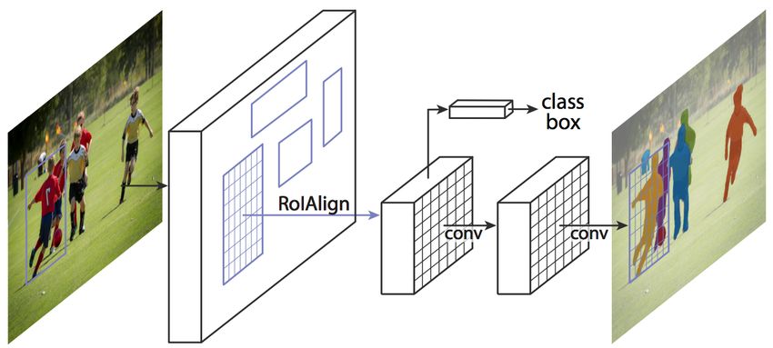
deep learning models, convolutional neural network(CNN)[3, 4, 5] has shown
outstanding performance in different high level computer vision task such
as image classification [6, 7, 8, 9, 10, 11, 12, 13, 14, 15], object detection
[16, 17, 18, 19, 20, 21, 22, 23, 24, 25, 26, 27, 28] etc. Though the advent
and success of AlexNet [6] turned the field of computer vision towards CNN
from traditional machine learning algorithms. But the concept of CNN was
not a new one. It started from the discovery of Hubel and Wiesel [29] which
explained that there are simple and complex neurons in the primary visual
cortex and the visual processing always starts with simple structures such as
oriented edges. Inspired by this idea, David Marr gave us the next insight
that vision is hierarchical [30]. Kunihiko Fukushima was deeply inspired by
the work of Hubel and Wiesel and built a multi-layered neural network called
Neocognitron [31] using simple and complex neurons. It was able to recognize
patterns in images and was spatial invariant. In 1989, Yann LeCun turned
the theoretical idea of Neocognitron into a practical one called LeNet-5 [32].
LeNet-5 was the first CNN developed for recognizing handwritten digits.
LeCun et al. used back propagation [33][11] algorithm to train his CNN.
The invention of LeNet-5 paved the way for the continuous success of CNN
in various high-level computer vision tasks as well as motivated researchers to
explore the capabilities of such networks for pixel-level classification problems
like image segmentation. The key advantage of CNN over traditional machine
learning methods is the ability to learn appropriate feature representations
for the problem at hand in an end-to-end training fashion instead of using
hand-crafted features that require domain expertise [34].
    Applications of image segmentation are very vast. From the autonomous
car driving [35] to medical diagnosis [36, 37], the requirement of the task
of image segmentation is everywhere. In this paper, we have tried to give
a survey of different image segmentation models based on CNN. Semantic
segmentation and instance segmentation of an image are discussed. Herein,
we have described comparative architectural details of different state-of-the-
art image segmentation models. Also, different aspects of those models are
presented in tabular form for clear understanding.

1.1. Contributions of this paper
    • Gives taxonomy and survey of the evolution of CNN based image seg-
      mentation.

   • Explores elaborately some CNN based popular state-of-the-art segmen-

                                       2
tation models.

   • Compares training details of those models to have a clear view of hyper-
     parameter tuning.

   • Compares the performance metrics of those state-of-the-art models on
     different datasets.

1.2. Organization of the Article
    Starting from the introduction in section 1, the paper is organized as
follows: In section 2, we have given background details of our work. In
sections 3 and 4, semantic segmentation and instance segmentation works
are discussed respectively with some subsections. In section 5, Panoptic
segmentation is presented in brief. The paper is concluded in section 6.

2. Background Details
2.1. Image Segmentation
    In computer vision, image segmentation is a way of segregating a digital
image into multiple regions according to the different properties of pixels.
Unlike classification and object detection, it is typically a low-level or pixel-
level vision task as the spatial information of an image is very important
for segmenting different regions semantically. Segmentation aims to extract
meaningful information for easier analysis. In this case, the image pixels
are labeled in such a way that every pixel in an image shares certain char-
acteristics such as color, intensity, texture, etc. [38, 39]. Mainly, image

                  Figure 1: Different types of image segmentation

                                        3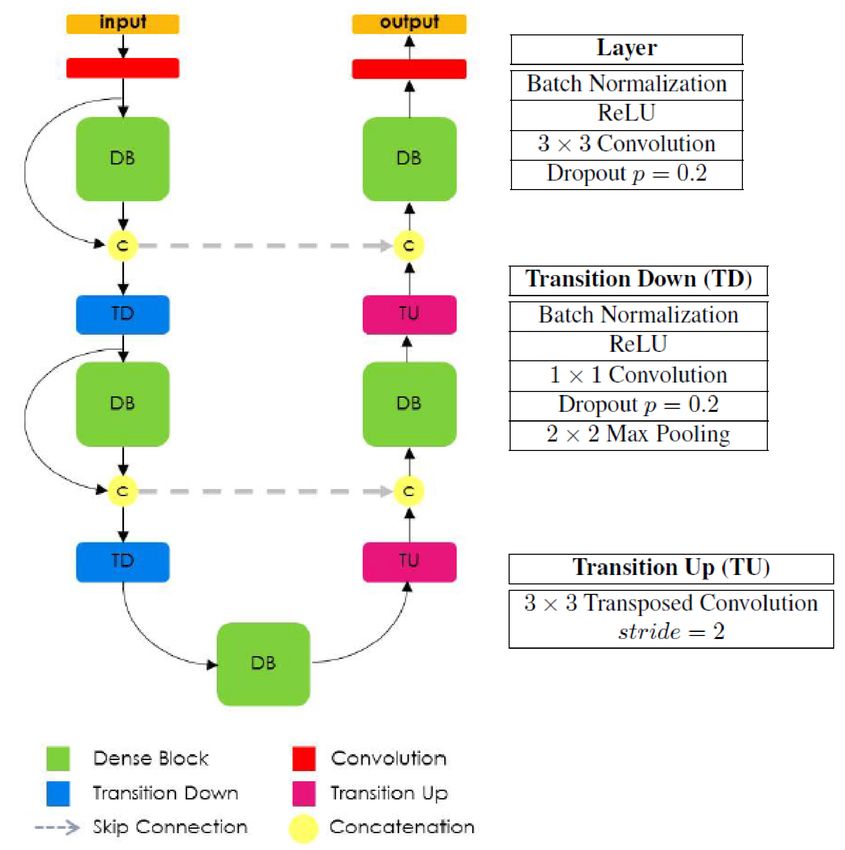
segmentation is of two types: semantic segmentation and instance segmen-
tation. Also, there is another type called panoptic segmentation[40] which
is the unified version of two basic segmentation processes. Figure 1 shows
different types of segmentation and figure 2 shows the same with examples.

         Figure 2: An example of different types of image segmentation [40]

2.2. Why CNN?
    The task of segmenting an image is not a new field of computer vision.
Various researchers are addressing this task in different way using tradi-
tional machine learning algorithms like in [41, 42, 43] with the help various
technique such as thresholding [44], region growing [45, 46], edge detection
[47, 48, 49], clustering [50, 51, 52, 53, 54, 55, 56, 57], super-pixel [58, 59]
etc for years. Most of the successful works are based on handcrafted ma-
chine learning features such as HOG [60, 61, 62, 63], SIFT [64, 65] etc. First
of all, feature engineering needs domain expertise and the success of those
machine learning-based models was slowed down around the era when deep
learning was started to take over the world of computer vision. To give a
outstanding performance, deep learning only needs data and it does not need
any traditional handcrafted feature engineering techniques. Also, traditional
machine learning algorithm can not adjust itself for a wrong prediction. On
the other hand, deep learning has that capability to adapt itself according

                                         4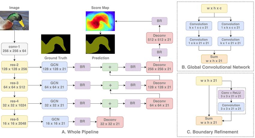
to the predicted result. Among different deep learning algorithms, CNN got
tremendous success in different fields of computer vision as well as grab the
area of image segmentation [66, 67, 68].
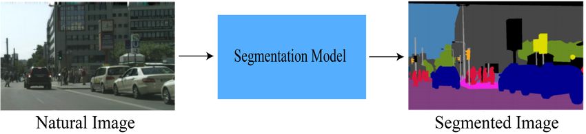
3. Semantic Segmentation
Semantic segmentation describes the process of associating each pixel of
an image with a class label [69]. Figure 3 shows the black-box view of seman-
tic segmentation. After the success of AlexNet in 2012, we have got different
successful semantic segmentation models based on CNN. In this section, we
are going to survey the evolution of CNN based semantic segmentation mod-
els. In addition, we are going to bring up here an elaborate exploration of
some state-of-the-art models.
Figure 3: The process of semantic segmentation[40]
3.1. Evolution of CNN based Semantic Segmentation Models:
The application of CNN in semantic segmentation models has started
with a huge diversity. In [70], the authors have used multi-scale CNN for
scene labeling and achieve state-of-the-art results in the Sift flow [71], the
Bercelona dataset [72] and the Standford background dataset [73]. R-CNN
[74] used selective search [75] algorithm to extract region proposals first and
then applied CNN upon each proposal for PASCAL VOC semantic segmenta-
tion challenge [76]. R-CNN achieved record result over second order pooling
(O2 P ) [77] which was a leading hand-engineered semantic segmentation sys-
tem at that time. At the same time, Gupta et al. [63] used CNN along with
geocentric embedding on RGB-D images for semantic segmentation.
Among different CNN based semantic segmentation models, Fully Con-
volutional Network(FCN) [78], as discussed in section 3.2.1, gained the max-
imum attention and an FCN based semantic segmentation model trend has
emerged. Major changes in FCN which helped the model to achieve state
5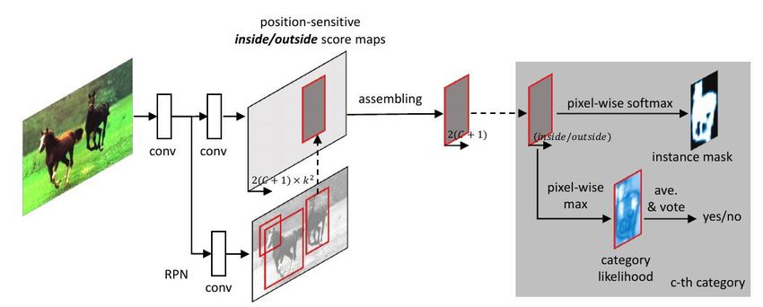
of the art result are the base model VGG16, bipolar interpolation technique
for up-sampling the final feature map and skip connection for combining low
layer and high layer features in the final layer for fine-grained semantic seg-
mentation. FCN has used only local information for semantic segmentation
but only local information makes semantic segmentation quite ambiguous.
To reduce ambiguity contextual information from the whole image is much
helpful. In [79] and [80] authors have used contextual features and achieved
state of the art performance. Recently, in [81], the authors have used fully
convolutional two stream fusion network for interactive image segmentation.
    Chen et al aggregate ‘atrous’ algorithm and conditional random (CRF)
field in semantic segmentation and proposed DeepLab [82] as discussed in
section 3.2.2. Later the authors have incorporated ‘Atrous Special Pyramid
Pooling (ASPP)’ in DeepLabv2 [83]. DeepLabv3[84] has gone further and
used a cascaded deep ASPP module to incorporate multiple contexts. All
three versions of DeepLab have achieved good results.
    Deconvnet [85] used convolutional network followed by hierarchically op-
posite de-convolutional network for semantic segmentation as discussed in
section 3.2.3. Ronneberger et al used a U-shaped network called U-Net [86]
which has a contracting and an expansive pathway to approach semantic
segmentation. Contracting path extracts feature maps and reduces spatial
information as a traditional convolution network. Expansive pathway takes
the contracted feature map as input and apply an up-convolution. In each
step of the expansive pathway, the network concatenates the reduced up-
convolved feature map with the corresponding cropped feature map from
the contracting pathway. In this way, U-Net incorporates both high-level
feature and low-level spatial information together for more precise segmen-
tation. Section 3.2.4 discussed the model in more detail. Recently, in [87],
the authors have used U-Net with multiRes block for multimodal biomedical
image segmentation and got better result than using classical U-Net. SegNet
[88] is a encoder-decoder network for semantic segmentation. The encoder
is a basic VGG16 network excluding FC layers. The decoder is identical to
encoder but the layers are hierarchically opposite. The Decoder used convo-
lution and unpooling operation to get a feature map of a size similar to input
image for precise localization of the segmented objects. SegNet is discussed
in section 3.2.7. The basic architectural intuition of U-Net, Deconvnet, and
SegNet are similar except some individual modifications. The second half of
those architectures is the mirror image of the first half.
    Liu et al mixed the essence of global average pooling and L2 normalization

                                      6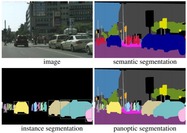
layer in FCN [78] architecture, and proposed ParseNet [89] to achieve state
of the art result in various datasets. Zhao et al. proposed Pyramid Scene
Parsing Network(PSPNet) [90]. They have used Pyramid Pooling Module
on top of the last extracted feature map to incorporate global contextual
information for better segmentation. Peng et al used the idea of global
convolution using a large kernel to apply the advantage of both local and
global features [91]. Pyramid Attention Network (PAN) [92], ParseNet [89],
PSPNet[90] and GCN[91] have used global context information with local
feature to have better segmentation. Sections 3.2.6, 3.2.9 and 3.2.8 will
discuss those models in detail.
    Fully convolutional DenseNet [10] is used to address semantic segmenta-
tion in [93, 94]. DeepUNet [95], a ResNet based FCN, used to segment sea
land. At the same time, ENet[96], ICNet[97] are used as real-time seman-
tic segmentation models for the autonomous vehicles. Some recent works
[98, 99, 100] have used combination of encoder-decoder architecture and di-
lated convolution for better segmentation. Kirillov et al.[101] used point-
based rendering in DeepLabV3[84] and in semanticFPN [102] and produce
state-of-the-art semantic segmentation model.

3.2. Some popular state-of-the-art semantic segmentation models:
    In this section, we are going to explore architectural details of some state
of the art CNN based semantic segmentation models in detail.

3.2.1. FCN:
    Long et al. proposed the idea of Fully Convolutional Network(FCN)
[78] to address the semantic segmentation task. They have used AlexNet[6],
VGGNet[8] and GoogleNet[9], pre-trained on ILSVRC [103] data, as base
model. They transferred these models from classifiers to dense FCN by sub-
stituting fully connected layers with 1 × 1 convolutional layers and append a
1 × 1 convolution with channel dimension 21 to predict scores for each of the
PASCAL VOC [104] class (including background). This process produces
a class presence heat map in low resolution. The authors have experienced
that among FCN-AlexNet, FCN-VGG16 and FCN-GoogLeNet, FCN-VGG16
gave the highest mean IU(56.0 %) on PASCAL VOC 2011 validation dataset.
So they choose the FCN-VGG16 network for further experiments. As the
network produces coarse output locations, the authors used bilinear inter-
polation to up-sample the coarse output 32× to make it pixel dense. But

                                       7
Figure 4: Architecture of FCN32s, FCN16s, FCN8s

this up-sampling was not enough for fine-grained segmentation. So the au-
thors have used skip connection[105] to combine the final prediction layer
and feature-rich lower layers of VGG16 and call this combination as deep
jet. Figure 4 shows different deep jet : FCN-16s and FCN-8s and FCN-32s.
The authors have shown that FCN-8s gave the best result in PASCAL VOC
2011 & 2012 [104] test dataset and FCN-16s gave the best result on both
NYUDv2 [106] & SIFT Flow [71] datasets.

3.2.2. DeepLab:
    Chen et al. has brought together methods from Deep Convolutional
Neural Network(DCNN) and probabilistic graphical model, and produced
DeepLab [82] to address semantic segmentation. DeepLab achieved 71.6%
IOU accuracy in the test set of the PASCAL VOC 2012 semantic segmenta-
tion task. The authors have faced two technical difficulties in the application
of DCNN to semantic segmentation: down sampling and spatial invariance.
To handle the first problem, the authors have employed ‘atrous’ (with holes)
[107] algorithm for efficient dense computation of CNN. Figure 5a and 5b
shows atrous algorithm in 1-D and in 2-D. To handle the second problem,
they have applied a fully connected pairwise conditional random field (CRF)
to capture fine details. In addition, the authors have reduced the size of the
receptive field 6× than the original VGG16 [8] network to reduce the time
consumption of the network and also used multi-scale prediction for bet-
ter boundary localization. The authors again modified the DeepLab using
Atrous Special Pooling Pyramid (ASPP) to aggregate multi-scale features

                                      8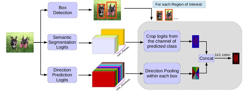
(a)                                (b)

Figure 5: Illustration of atrous algorithm (a) in 1-D, when kernel size=3, input-stride=2
and output-stride=1 [82] and (b) in 2-D, when kernel size 3 × 3, with rate 1, 6 and 24 [84]

for better localization and proposed DeepLabv2 [83]. Figure 6 shows ASPP.
This architecture used both ResNet [10]and VGGNet[8] as base network. In
DeepLabv3[84], to incorporate multiple contexts in the network, the authors
have used cascaded modules and have gone deeper especially with the ASPP
module.

                     Figure 6: Atrous Spatial Pooling Pyramid [84]

3.2.3. Deconvnet:
    Deconvnet [85] proposed by Noh et al., has a convolutional and de-
convolutional network. The convolutional network is topologically identical
with the first 13 convolution layers and 2 fully connected layers of VGG16[8]
except for the final classification layer. As in VGG16, pooling and recti-
fication layers are also added after some of the convolutional layers. The
De-convolutional network is identical to the convolutional network but hier-
archically opposite. It also has multiple series of deconvolution, un-pooling
and rectification layers. All the layers of convolutional and de-convolutional
network extract feature maps except the last layer of the de-convolutional
network which generates pixel-wise class probability maps of the same size

                                            9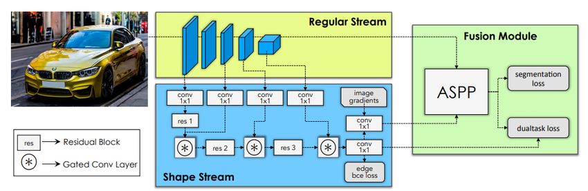
as the input image. In the deconvolutional network, the authors have ap-
plied unpooling which is the reverse operation of the pooling operation of the
convolutional networks to reconstruct the original size of activation. Follow-
ing [7][108], unpooling is done using max-pooling indices which are stored
at the time of convolution operation in the convolutional network. To den-
sify enlarged but sparse un-pooled feature maps, convolution like operation
is done using multiple learned filters by associating single input activation
with multiple outputs. Unlike FCN, the authors applied their network on
object proposals extracted from the input image and produced pixel-wise
prediction. Then they have aggregated outputs of all proposals to the orig-
inal image space for segmentation of the whole image. This instance wise
segmentation approach handles multi-scale objects with fine detail and also
reduces training complexity as well as memory consumption for training. To
handle the internal covariate shift in the network, the authors have added
batch normalization [109] layer on top of convolutional and de-convolutional
layers. The architecture of Deconvnet is shown in figure 7.

         Figure 7: Convolution-Deconvolution architecture of Decovnet [85]

3.2.4. U-Net:
    U-Net [86]is a U-shaped semantic segmentation which has a contracting
path and an expansive path. Every step of the contracting path consists
of two consecutive 3 × 3 convolutions followed by ReLU nonlinearity and
max-pooling using 2 × 2 window with stride 2. During the contraction, the
feature information is increased while spatial information is decreased. On
the other hand, every step of the expansive path consists of up-sampling of
feature map followed by a 2×2 up-convolution. This reduces the feature map
size by a factor of 2. Then the reduced feature map is concatenated with
the corresponding cropped feature map from the contracting path. Then

                                        10
two consecutive 3 × 3 convolution operations are applied followed by ReLU
nonlinearity. In this way, the expansive pathway combines the features and
spatial information for precise segmentation. The architecture of U-Net is
shown in figure 8.
Figure 8: Contracting and expansive architecture of U-Net[86]
3.2.5. Dialatednet:
Traditional CNN, used for classification tasks, loses resolution in its way
and it is not suitable for dense prediction. Yu and Koltun have introduced a
modified version of traditional CNN, called dialated convolution or Dialated-
Net [110], to accumulate multi-scale contextual information systematically
for better segmentation without suffering the loss of resolution. Dialated-
Net is like a rectangular prism of convolutional layers, unlike conventional
pyramidal CNN. Without losing any spatial information, it can support the
exponential expansion of receptive fields as shown in figure 9.
3.2.6. ParseNet:
Liu et al proposed an end-to-end architecture called ParseNet [89] which
is an improvement of Fully Convolution Neural Network. The authors have
added global feature or global context information for better segmentation.
11Figure 9: (a) 1-dialatednet with receptive field 3 × 3, (b) 2-dialatednet with receptive field
7 × 7 and (c)-dialatednet with receptive field 15 × 15 [110]
.
In figure 10, the model description of ParseNet is shown. Till convolutional
feature map extraction, the ParseNet is the same as FCN [78]. After that,
the authors have used global average pooling to extract global contextual
information. Then the pooled feature maps are un-pooled to get the same
size as input feature maps. Now, the original feature maps and un-pooled
feature maps are combined for predicting the final classification score. As
the authors have combined two different feature maps from two different
layers of the network, those feature maps would be different in scale and
norm. To make the combination work, they have used two L2 normalization
layers: one after global pooling and another after the original feature map
extracted from FCN simultaneously. This network achieved state-of -the-art
performance on ShiftFlow [71], PASCAL-context [111] and near the state of
the art on PASCAL VOC 2012 dataset.
Figure 10: ParseNet Model Design [89]
123.2.7. SegNet:
SegNet [88] has encoder-decoder architecture followed by a final pixel-wise
classification layer. The encoder network has 13 convolutional layers as in
VGG16 [8] and the corresponding decoder part also has 13 de-convolutional
layers. The authors did not use fully connected layers of VGG16 to re-
tain the resolution in the deepest layer and also to reduce the number of
parameters from 134M to 14.7M. In each layer in the encoder network, a
convolutional operation is performed using a filter bank to produce feature
maps. Then, to reduce internal covariate shift the authors have used batch
normalization [112] [113] followed by ReLU [114] nonlinearity operation. Re-
sulting output feature maps are max-pooled using a 2 × 2 non-overlapping
window with stride 2 followed by a sub-sampling operation by a factor of
2. A combination of max-pooling and sub-sampling operation achieves bet-
ter classification accuracy but reduces the feature map size which leads to
lossy image representation with blurred boundaries which is not ideal for
segmentation purposes where boundary information is important. To retain
boundary information in the encoder feature maps before sub-sampling, Seg-
Net stores only the max-pooling indices for each encoder map. For semantic
segmentation, the output image resolution should be the same as the input
image. To achieve this, SegNet does up-sampling in its decoder using the
stored max-pooling indices from the corresponding encoder feature map re-
sulting high-resolution sparse feature map. To make the feature maps dense,
the convolution operation is performed using a trainable decoder filter bank.
Then the feature maps are batch normalized. The high-resolution output
feature map produced form final decoder is fed into a trainable multi-class
softmax classifier for pixel wise labeling. The architecture of SegNet is shown
in figure 11.
Figure 11: Encoder-decoder architecture of SegNet[88]
133.2.8. GCN:
Like ParseNet, Global Convolution Network [91] has also used global fea-
tures along with local features to make the pixel-wise prediction more accu-
rate. The task of semantic segmentation is the combination of classification
Figure 12: Pipeline network of GCN [91]
and localization tasks. These two tasks are contradictory in nature. The
classification should be transformation invariant and localization should be
transformation sensitive. Previous state-of-the-art models focused on local-
ization more than classification. In GCN, the authors did not use any fully
connected layers or global pooling layers to retain spatial information. On
the other hand, they have used a large kernel size (global convolution) to
make their network transformation invariant in the case of pixel-wise clas-
sification. To refine the boundary further the authors have used Boundary
Refinement (BR) block. As shown in figure 12, ResNet is used as a backbone.
GCN module is inserted in the network followed by the BR module. Then
score maps of lower resolution are up-sampled with a deconvolution layer,
and then added up with higher ones to generate new score maps for final
segmentation.
3.2.9. PSPNet:
Pyramid Scene Parsing Network(PSPNet) [90], proposed by Zhao et al.,
has also used global contextual information for better segmentation. In this
14model, the authors have used Pyramid Pooling Module on top of the last fea-
ture map extracted using dilated FCN. In Pyramid Pooling Module, feature
maps are pooled using 4 different scales corresponding to 4 different pyramid
levels each with bin size 1×1, 2×2, 3×3 and 6×6. To reduce dimension, the
Figure 13: PSPNet Model Design [90]
pooled feature maps are convolved using 1 × 1 convolution layer. The out-
puts of the convolution layers are up-sampled and concatenated to the initial
feature maps to finally contain the local and the global contextual informa-
tion. Then, they are again processed by a convolutional layer to generate the
pixel-wise predictions. In this network, the pyramid pooling module observes
the whole feature map in sub-regions with a different locations. In this way,
the network understands a scene better which also leads to better semantic
segmentation. In figure 13, the architecture of PSPNet is shown.
3.2.10. FC-DenseNet:
DenseNet [10] is a CNN based classification network that contains only
a down-sampling pathway for recognition. Jégou et al. [115] has extended
DenseNet by adding an up-sampling pathway to regain the full resolution of
the input image. To construct the up-sampling pathway, the authors followed
the concept of FCN. They have referred the down-sampling operation of
DenseNet as Transition Down (TD) and up-sampling operation in extended
DenseNet as Transition UP (TU) as shown in figure 14. The rest of the
convolutional layers follows the sequence of Batch Normalization, ReLU, 3×3
convolution and dropout of 0.2 as shown in the top right block in figure 14.
The up-sampling pathway used the sequence of dense block [10] instead of
convolution operation of FCN and used transposed convolution as an up-
sampling operation. The up-sampling feature maps are concatenated with
the feature maps derived from corresponding layers of the down-sampling
15pathway. In figure 14 these long skip connections are shown in yellow circle.
Figure 14: Architecture of Fully Convolutional DenseNet for semantic segmentation with
some building blocks[115]
3.2.11. Gated-SCNN:
Figure 15: Architecture of Gated Shape CNN for semantic segmentation [94]
Takikawa et al. proposed Gated - Shape CNN(GSCNN) [94] for Seman-
tic Segmentation. As shown in figure 15, GSCNN consists of two streams of
networks: regular stream and shape stream. The regular stream is a classical
CNN for processing semantic region information. Shape stream consists of
16multiple Gated Convolution Layer (GCL) which process boundary informa-
tion of regions using low-level feature maps from the regular stream. Outputs
of both streams are fed into a fusion module. In fusion modules, both out-
puts are combined using Atrous Special Pyramid Pooling [83] module. The
use of ASPP helps their model to preserve multi-scale contextual informa-
tion. Finally, the Fusion module produced semantic region of objects with a
refined boundary.
3.3. Discussion
From the year 2012, different CNN based semantic segmentation models
have emerged in successive years to date. In subsection 3, we have described
major up-gradation in the networks of various state-of-the-art models for
better semantic segmentation. Among different models, Fully Convolutional
Network (FCN) has set a path for semantic segmentation. Various models
have used FCN as their base model. DeepLab and its versions have used
atrous algorithm in different ways. SegNet, DeconvNet, U-Net have a simi-
lar architecture where the second part of those architectures is hierarchically
opposite of the first half. ParseNet, PSPNet, and GCN have addressed se-
mantic segmentation with respect to contextual information. FCDenseNet
used top-down /bottom-up approach to incorporate low-level features with
high-level features. So, the performance of a semantic segmentation model
depends on the internal architecture of a network as well as other aspects
such as the size of the data set, number of semantically annotated data, dif-
ferent training hyperparameters (such as learning rate, momentum, weight
decay), optimization algorithm, loss function, etc. In this section, we have
given different comparative aspects of each model in tabular form.
3.3.1. Optimization Details of Different State-of-the-art Semantic Segmen-
tation Models:
Table 1 shows different optimization details of different models where we
can see that the success of a model not only depends on the architecture.
Table 2 presents base network (pre-trained on ImageNet [116] dataset), data
pre-processing technique (basically data augmentation) and different loss
function used for different models. Table 3 has briefly shown some important
features of each model.
17Table 1: Optimization details of different state-of-the-art semantic segmentation models
Name of Optimization Mini Learning Rate Momentum Weight
the model Algorithm Batch Size Decay
FCN- SGD [117] 20 images 0.0001 0.9 0.0016 or
VGG16 0.0625
[78]
DeepLab SGD 20 images initially 0.001 (0.01 0.9 0.0005
[82] for final classification
layer), increasing it
by 0.1 at every 2000
iteration.
Deconvnet SGD - 0.01 0.9 0.0005
[85]
U-Net [86] SGD single image 0.99
DialatedNet SGD 14 images 0.001 0.9 -
[110]
ParseNet SGD 1e − 9 0.9
[89]
SegNet [88] SGD 12 images 0.1 0.9
GCN [91] SGD Single 0.99 0.0005
image
PSPNet [90] SGD 16 images ‘poly’ learning rate 0.9 0.0001
with base learning rate
of 0.01 and power to
0.9
FC- SGD initially 1e − 3 with 1e − 4
DenseNet103 an exponential decay of
[115] 0.995
Gated- SGD 16 1e − 2 with polynomial 0
SCNN decay policy
[94]
3.3.2. Comparative Performance of State-of-the-art Semantic Segmentation
Models:
In this section, we are going to show the comparative result of different
state-of-the-art semantic segmentation modelson the various datasets. The
performance metric used here is mean average precision (mAP) as Intersec-
tion over union(IoU) threshold
4. Instance Segmentation
Like semantic segmentation, the applicability of CNN has been spread
over instance segmentation too. Unlike semantic segmentation, instance seg-
mentation masks each instance of an object contained in an image indepen-
dently [126, 127]. The task of object detection and instance segmentation
18Table 2: Base Model, data preprocessing technique and loss functions of different state-
of-the-art semantic segmentation models.
Name of Base Data pre-processing Loss
the Network Funtion
model
FCN- AlexNet[6], VGGnet[8], Per-pixel multinomial logistic
VGG16 GoogLeNet[9] (All pre-trained loss
[78] on ILSVRC dataset [103])
DeepLab VGG16 [8] pre-trained on Data augmentation using extra Sum of cross-entropy loss
[82] ILSVRC dataset annotated data of [118]
Deconvnet VGG16 pre-trained on ILSVRC Data augmentation using extra
[85] dataset annotated data of [118]
U-Net [86] FCN [78] Data augmentation by applying Cross entropy loss
random elastic deformation to
the available training images
DialateNet VGG16 [8] Data augmentation using extra
[110] annotated data of [118]
ParseNet FCN [78]
[89]
SegNet VGG16 [8] Local contrast normalization to Cross
[88] RGB data entropy loss
GCN [91] ResNet152 [10] as feature net- Semantic Boundaries Dataset
work and FCN-4 [78] as segmen- [118] is used as auxiliary dataset
tation network
PSPNet Pretrained ResNet [10] Data augmentation: random Four losses:
[90] mirror and random resize be- • Additional loss for initial re-
tween 0.5 and 2, random rota- sult generation
tion between -10 and 10 degrees, • Final loss for learning the
random Gaussian blur residue later
• Auxiliary loss for shallow lay-
ers
• Master branch loss for final
prediction
FC- DensNet [10] Data augmentation using ran-
DenseNet dom cropping and vertical flip-
[115] ping
Gated- ResNet101[10] and • Segmentation loss for regular
SCNN WideResNet[119] stream
[94] • Dual task loss for shape
stream
•• Standard binary cross en-
tropy loss for boundary refine-
ment
•• Standard cross entropy for
semantic segmentation
are quite correlated. In object detection, researchers use the bounding box
to detect each object instance of an image with a label for classification. In-
stance segmentation put this task one step forward and put a segmentation
mask for each instance.
Concurrent to semantic segmentation research, instance segmentation re-
search has also started to use the convolutional neural network(CNN) for
better segmentation accuracy. Herein, we are going to survey the evolution
of CNN based instance segmentation models. In addition, we are going to
bring up here an elaborate exploration of some state-of-the-art models for
instance segmentation task.
19Table 3: Some important features of different state-of-the-art semantic segmentation mod-
els
Model Important Features
FCN-VGG16 • Dropout is used to reduce overfitting
• End to end trainable
DeepLab • End to end trainable
• Piecewise training for DCNN and CRF
• Inference time during testing is 8frame per second
• Used Atrous Special Pyramid Pooling module for aggregating multi-scale features
Deconvnet • Used edge-box to generate region proposal
• Used Batch Normalization to reduce internal covariate shift and removed dropout
• Two-stage training for easy examples and for more challenging examples
• End to end trainable
• Drop-out layer is used at the end of the contracting path
U-Net • End to end trainable
• Inference time for testing was less than 1 sec per image
DialatedNet Two stage training:
• Front end module with only dilated convolution
• Dilated convolution with multi-scal context module
ParseNet • End to end trainable
• Batch Normalization is used
• Drop-out of 0.5 is used in deeper layers
SegNet • Different Ablation study
GCN • Large Kernel Size
• Included Global Contextual information
PSPNet • End to end training
• Contains dialated convolution
• Batch normalization
• Used pyramid pooling module for aggregating multi-scale features
FC-DensNet • Initialized the model with HeUniform[120] and trained it with RMSprop
dataset[121]
• Used dropout of 0.2
• Used the model parameters efficiently
Gated -SCNN • End to end trainable
• Applied ablation study
4.1. Evolution of CNN based Instance Segmentation Models:
CNN based instance segmentation has also started its journey along with
semantic segmentation. As we have mentioned in section 4 that instance
segmentation task only adds a segmentation mask to the output of object
detection task. That is why most of the CNN based instance segmentation
models have used different CNN based object detection models to produce
better segmentation accuracy and to reduce test time.
Hariharan et al. have followed the architecture of R-CNN [74] object
detector and proposed a novel architecture for instance segmentation called
Simultaneous Detection and Segmentation(SDS) [127] which is a 4 step in-
stance segmentation model as described in section 4.2.1.
Till this time CNN based models have only used the last layer feature map
20Table 4: Comparative accuracy of different semantic segmentation models in terms of
mean average precision (mAP) as Intersection over Union (IoU)
Model Year Used Dataset mAP as IoU
FCN-VGG16 [78] 2014 Pascal VOC 2012 [76] 62.2%
DeepLab[82] 2014 Pascal VOC 2012 71.6%
Deconvnet[85] 2015 Pascal VOC 2012 72.5%
U-Net[86] 2015 ISBI cell tracking challenge 2015 92% on PhC-U373 and 77.5% on
DIC-HeLa dataset
DialatedNet [110] 2016 Pascal VOC 2012 73.9%
ParseNet [89] 2016 • ShiftFlow [71] 40.4%
• PASCAL- Context [111] 36.64%
• Pascal VOC 2012 69.8%
SegNet [88] 2016 • CamVid road scene segmenta- 60.10%
tion [122]
• SUN RGB-D indoor scene 31.84%
segmentation[123]
GCN[91] 2017 • PASCAL VOC 2012 82.2%
•Cityscapes [124] 76.9%
PSPNet [90] 2017 • PASCAL VOC 2012 85.4%
• Cityscapes 80.2%
FC-DenseNet103 [115] 2017 • CamVid road scene segmenta- 66.9%
tion
• Gatech[125] 79.4%
Gated-SCNN [94] 2019 • Cityscapes 82.8%
for classification, detection and even for segmentation. In 2014, Hariharan
et al. have again proposed a concept called Hyper-column [128] which has
used the information of some or all intermediate feature maps of a network
for better instance segmentation. The authors added the concept of Hyper-
column to SDS and their modified network achieved better segmentation
accuracy
Different object detector algorithms such as R-CNN, SPPnet [17], Fast R-
CNN [18] have used two stages network for object detection. The first stage
detects object proposals using Selective Search [75] algorithm and second
stage classify those proposals using different CNN based classifier. Multi-
box [129, 130], Deepbox [131], Edgebox [132] have used CNN based proposal
generation method for object detection. Faster R-CNN [19] have used CNN
based ‘region proposal network (RPN)’ for generating box proposal. How-
ever, the mode of all these proposal generations is using a bounding box
and so the instance segmentation models. In parallel to this, instance seg-
mentation algorithms such as SDS and Hyper column have used Multi-scale
Combinatorial Grouping (MCG)[133] for region proposal generation. Deep-
Mask [134], as discussed in section 4.2.2, has also used CNN based RPN as
Faster R-CNN to generate region proposals so that the model can be trained
21end to end.
Previous object detection and instance segmentation modules such as
[74],[17],[18],[19] [127],[128],[134] etc. have used computationally expensive
external methods for generating object level or mask level proposals like
Selective Search, MCG, CPMC [77], RPN etc. Dai et al. [135] break the
tradition of using a pipeline network and did not use any external mask pro-
posal method. The authors have used a cascaded network for incorporating
features from different CNN layers for instance segmentation. Also, the shar-
ing of convolution features leads to faster segmentation models. Detail of the
network is discussed in section 4.2.3.
In papers [136], [137], [80], [17], [138], [128], [78], [139] researchers used
contextual information and low level features into CNN in various ways for
better segmentation. Zagoruko et al. [140] has also used those ideas by
integrating skip connection, foveal structure and integral loss in Fast R-CNN
[18] for better segmentation. Further description is given in section 4.2.4.
SDS, DeepMask, Hyper-columns have used feature maps from top layers
of the network for object instance detection which leads to coarse object mask
generation. Introduction of skip connection in [141, 142, 143, 140] reduces
the coarseness of masks which is more helpful for semantic segmentation
rather instance segmentation. Pinheiro et. al.[144] have used their model to
generate a coarse feature map using CNN and then refined those models to
get pixel-accurate instance segmentation masks using a refinement model as
described in section 4.2.5.
Traditional CNNs are translation invariant i.e images with the same prop-
erties but with different contextual information will score the same classifi-
cation score. Previous models, specially FCN, used a single score map for
semantic segmentation. But for instance segmentation, a model must be a
translation variant so that the same image pixel of different instances having
different contextual information can be segmented separately. Dai et al [21]
integrated the concept of relative position into FCN to distinguish multiple
instances of an object by assembling a small set of score maps computed
from the different relative positions of an object. Li et al [145] extended the
concept of [21] and introduced two different position-sensitive score maps
as described in section 4.2.7. SDS, Hypercolumn, CFM[146], MNC [135],
MultiPathNet[140] used two different subnetworks for object detection and
segmentation which prevent the models to become an end to end trainable.
On the other hand [147],[148] extends instance segmentation by grouping or
clustering FCNs score map which involves a large amount of post-processing.
22[145] introduced a joint formulation of classification and segmentation mask-
ing subnets in an efficient way.
While [149, 150, 151, 152] have used semantic segmentation models, Mask
R-CNN [20] extends the object detection model Faster R-CNN by adding a
binary mask prediction branch for instance segmentation.
The authors of [153], [154] has introduced direction features to predict
different instances of a particular object. [153] has used template matching
technique with direction feature to extract the center of an instance whereas
[154] followed the assembling process of [145, 21] to get instances.
[155, 156, 150, 128] have used features form intermediate layers for better
performance. Liu et al.[157] have also used the concept of feature propagation
from a lower level to top-level and built a state-of-the-art model based on
Mask R-CNN as discussed in section 4.2.10.
Object detection using the sliding window approach gave us quite suc-
cessful work such as Faster R-CNN, Mask R-CNN, etc. with refinement step
and SSD[23], RetinaNet[26] without using refinement stage. Though sliding
window approach is popular in object detection but it was missing in case
of instance segmentation task. Chen et al. [158] have introduced dense in-
stance segmentation to fill this gap and introduced TensorMask. Recently,
Kirillov et al.[101] used point-based rendering in Mask R-CNN and produce
state-of-the-art instance segmentation model.
4.2. Some State-of-the-art Instance Segmentation Models:
In this section, we are going to elaborately discuss some state-of-the-art
CNN based instance segmentation models.
4.2.1. SDS:
Simultaneous Detection and Segmentation (SDS) [127] model consists of
4 steps for instance segmentation. The steps are proposal generation, feature
extraction, region classification, and region refinement respectively. On input
image, the authors have used Multi-scale Combinatorial Grouping(MCG)
[133] algorithm for generating region proposals. Then each region proposals
are fed into two CNN based sibling networks. As shown in figure 16, the
upper CNN generates a feature vector for bounding box of region proposals
and the bottom CNN generates a feature vector for segmentation mask. Two
feature vectors are then concatenated and class scores are predicted using
SVM for each object candidate. Then non-maximum suppression is applied
on the scored candidates to reduce the set of same category object candidates.
23Figure 16: Architecture of SDS Network[127]
Finally, to refine surviving candidates CNN feature maps are used for mask
prediction.
4.2.2. DeepMask:
DeepMask [134] used CNN to generate segmentation proposals rather
than less informative bounding box proposal algorithms such as Selective
Search, MCG, etc. DeepMask used VGG-A[8] model (discarding last max-
Figure 17: Model illustration of DeepMask [134].
pooling layer and all fully connected layers) for feature extraction. As shown
in figure 17, the feature maps are then fed into two sibling branches. The
top branch which is the CNN based object proposal method of DeepMask
predicts a class-agnostic segmentation mask and bottom branch assigns a
score for estimating the likelihood of patch being centered on the full object.
The parameters of the network are shared between the two branches.
4.2.3. Multi-task Network Cascades (MNC):
Dai et al. [135] used a network with the cascaded structure to share
convolutional features and also used region proposal network (RPN) for bet-
ter instance segmentation. The authors have decomposed the instance seg-
24mentation task into three sub tasks: instance differentiation (class agnostic
bounding box generation for each instance), mask estimation(estimated a
pixel-level mask/instance ) and object categorization (instances are labeled
categorically). They proposed Multi-task Network Cascades (MNC) to ad-
dress these sub-tasks in three different cascaded stages to share convolutional
features. As shown in figure 18, MNC takes an arbitrary sized input which
is a feature map extracted using VGG16 network. Then at the first stage,
the network generates object instances from the output feature map as class
agnostic bounding boxes with an abjectness score using RPN. Shared convo-
lutional features and output boxes of stage-1 then go to the second stage for
regression of mask level class-agnostic instances. Again, shared convolutional
features and output of the previous two stages are fed into the third stage
for generating category score for each instance.
Figure 18: Three stage architecture of Multi-task Network Cascades [135].
4.2.4. MultiPath Network:
Zagoruko et al. integrate three modifications in the Fast R-CNN object
detector and proposed Multipath Network [140] for both object detection
and segmentation tasks. Three modifications are skip connections, foveal
structure, and integral loss. Recognition of small objects without context is
difficult. That is why, in [136], [137], [80], [17], [159], the researcher used con-
textual information in various ways in CNN based model for better classifica-
tion of objects. In Multipath Network, the authors have used four contextual
regions called foveal regions. The view size of those regions are 1×, 1.5×,
2×, 4× of the original object proposal. On the other hand, researchers of
[138], [128], [78], [139] has used feature from higher-resolution layers of CNN
25for effective localization of small objects. In Multipath Network, the authors
have connected third, fourth and fifth convolutional layers of VGG16 to the
four foveal regions to use multi-scale features for better object localization.
Figure 19 shows the architectural pipeline of MultiPath Network. Feature
maps are extracted from an input image using the VGG16 network. Then
using skip connection those feature maps go to four different Foveal Region.
The output of those regions are concatenated for classification and bound-
ing box regression. The use of the DeepMask segmentation proposal helped
their model to be the 1st runner-up in MS COCO 2015 [160]detection and
segmentation challenges.
Figure 19: Architecture of MultiPath Network [140].
4.2.5. SharpMask:
DeepMask generates accurate masks for object-level but the degree of
alignment of the mask with the actual object boundary was not good. Sharp-
Mask [144] contains a bottom-up feed-forward network for producing coarse
semantic segmentation mask and a top-down network to refine those masks
using a refinement module. The authors have used feed-forward DeepMask
segmentation proposal network with their refinement module and named it
as SharpMask. As shown in figure 20, the bottom-up CNN architecture pro-
duces coarse mask encoding. Then the output mask encoding is fed into a
top-down architecture where a refinement module un-pool it using match-
ing features from the bottom-up module. This process continues until the
reconstruction of the full resolution image and the final object mask.
26Figure 20: Bottom-up/top-down architecture of SharpMask [144].
4.2.6. InstanceFCN:
The fully convolutional network is good for single instance segmentation
of an object category. But it can not distinguish multiple instances of an
object. Dai et al have used the concept of relative position in FCN and
proposed instance sensitive fully convolutional network (InstanceFCN) [21]
for instance segmentation. The relative position of an image is defined by a
k × k grid on a square sliding window. This produces a set of k 2 instance
sensitive score maps rather than one single score map as FCN. Then the in-
stance sensitive score maps are assembled according to their relative position
in a m × m sliding window to produce object instances. In DeepMask[134],
shifting sliding window for one stride leads to the generation of two different
fully connected channels for the same pixel which is computationally exhaus-
tive. In InstanceFCN, the authors have used the concept of local coherence
[161] which means sliding a window does not require different computations
for a single object. Figure 21 shows the architecture of InstanceFCN.
4.2.7. FCIs
InstanceFCN introduced position-sensitive score mapping to signify the
relative position of an object instance but the authors have used two dif-
27Figure 21: Architecture of Instance-sensitive fully convolutional network [21].
ferent sub networks for object segmentation and detection. Because of two
different networks, the solution was not end to end. Li et al. [145] pro-
posed the first end to end trainable fully convolutional network based model
in which segmentation and detection are done jointly and concurrently in a
single network by score map sharing as shown in figure 22. Also instead of
the sliding window approach, the model used box proposals following [19].
The authors have used two different position-sensitive score maps: position-
sensitive inside score maps and position sensitive outside score maps. These
two score maps depend on detection score and segmentation score of a pixel
in a given region of interests (RoIs) with respect to different relative position.
As shown in figure 22 RPN is used to generate RoIs. Then RoIs are used on
score maps to detect and segment object instances jointly.
4.2.8. Mask R-CNN
Mask R-CNN[20] contains three branches for predicting class, bounding-
box and segmentation mask for instances within a region of interest (RoI).
This model is the extension of Faster R-CNN. As Faster R-CNN, Mask R-
CNN contains two stages. In the first stage, it uses RPN to generate RoIs.
Then to preserve the spatial location, the authors have used RoIAlign in-
stead of RoIPool as in Faster R-CNN. In the second stage, it simultaneously
predicts a class label, a bounding box offset and a binary mask for each in-
dividual RoI. In Mask R-CNN, the prediction of binary mask for each class
was independent and it was not a multi-class prediction.
28Figure 22: Architecture of FCIs [145].
Figure 23: Architecture of Mask R-CNN[20].
4.2.9. MaskLab
MaskLab [154] has utilized the merits of both semantic segmentation and
object detection to handle instance segmentation. The authors have used
Faster R-CNN[19] (ResNet-101[10] based) for predicting bounding boxes for
object instances. Then they have calculated semantic segmentation score
maps for labeling each pixel semantically and direction score maps for pre-
dicting individual pixels direction towards the center of its corresponding
instance. Those score maps are cropped and concatenated for predicting a
coarse mask for target instance. The mask is then again concatenated with
hyper-column features[128] extracted from low layers of ResNet-101 and pro-
cessed using a small CNN of three layers for further refinement.
29Figure 24: Architecture of MaskLab [154].
4.2.10. PANet:
The flow of information in the convolutional neural network is very impor-
tant as the low-level feature maps are information-rich in terms of localization
and the high-level feature maps are rich in semantic information. Liu et al.
focused on this idea. Based on Mask R-CNN and Feature Pyramid Net-
work(FPN) [162], they have proposed a Path Aggregation Network (PANet)
[157] for instance segmentation. PANet used FPN as its base network to
extract features from different layers. To propagate the low layer feature
through the network, a bottom-up augmented path is used. Output of each
layer is generated using previous layers high-resolution feature map and a
coarse map from FPN using a lateral connection. Then an adaptive pooling
layer is used to aggregate features from all levels. In this layer, a RoIPool-
ing layer is used to pool features from each pyramid level and element wise
max or sum operation is used to fuse the features. As Mask R-CNN, the
output of the feature pooling layer goes to three branches for prediction of
the bounding box, prediction of the object class and prediction of the binary
pixel mask.
4.2.11. TensorMask
Previous instance segmentation models used methods in which the ob-
jects are detected using bounding box then segmentation is done. Chen et
al. have used the dense sliding window approach instead of detecting the
object in a bounding box named TensorMask [158]. The main concept of
this architecture is the use of structured high-dimensional (4D) tensors to
present mask over an object region. A 4D tensor is a quadruple of (V, U,
H, W). The geometric sub-tensor (H, W) represents object position and (V,
30Figure 25: Architecture of PANet [157].
U) represents the relative mask position of an object instance. Like fea-
ture pyramid network, TensorMask has also developed a pyramid structure,
called tensorbipyramid over a scale-indexed list of 4D tensors to acquire the
benefits of multi-scale.
4.3. Discussion:
In the previous subsection 4.2, we have presented important architectural
details of different state-of-the-art models. Among different models, some of
them are based on object detection models such as R-CNN, Fast R-CNN,
Faster R-CNN, etc. Some models are based on semantic segmentation mod-
els such as FCN, U-Net, etc. SDS, DeepMask, SharpMask, InstanceFCN
are based on proposal generation. InstanceFCN, FCIs, MaskLab calculate
position-sensitive score maps for instance segmentation. PANet emphasized
on feature propagation across the network. TensorMask used the sliding
window approach for dense instance segmentation. So, architectural differ-
ences help different models to achieve success in various instance segmen-
tation dataset. On the other hand, fine-tuning of hyper-parameters, data
pre-processing methods, choice of the loss function and optimization func-
tion, etc are also played an important role in the success of a model. In this
subsections, we are going to present some of those important features in a
comparative manner.
4.3.1. Optimization Details of State-of-the-art Instance Segmentation Mod-
els:
The training and optimization process is very crucial for a model to be-
come successful. Most of the state-of-the-art models used stochastic gradient
descent(SGD) [163] as an optimization algorithm with different initialization
31Table 5: Optimization details of different state-of-the-art instance segmentation models
Name of Optmization Mini Learning Rate Momentum Weight
the model Algorithm Batch Size Decay
DeepMask SGD 32 images 0.001 0.9 0.00005
[134]
MNC [135] SGD 1 images per 0.001 for 32k iteration,
GPU, total 8 0.0001 for next 8K itera-
GPUs are used tion
MultPath Net- SGD 4 images,1 im- initially 0.001, after 160k - -
work [140] age per GPU, iterations, it was reduced
each with 64 to 0.0001
object propos-
als
SharpMask SGD 1e−3
[144]
InstanceFCN SGD 8 images each 0.001 for initial 32k iter- 0.9 0.0005
[21] with 256 sam- ations and 0.0001 for the
pled windows, next 8k.
1 image/GPU
FCIs [145] SGD 8 im- 0.001 for the first 20k and
ages/batch, 0.0001 for the next 10k it-
1 image per erations
GPU
Mask R-CNN SGD 16 im- 0.02 for first 160k iteration 0.0001 0.9
[20] ages/batch, and 0.002 for next 120k it-
2 images per erations
GPU
PANet [157] SGD 16 images 0.02 for 120k iterations 0.0001 0.9
and 0.002 for 40k itera-
tions
TensorMask SGD 16 images, 2 0.02 with linear warm- 0.9 0.0005
[158] images per up[163] of 1k iteration
GPU
of corresponding hyper parameters such as mini-batch size, learning rate,
weight decay, momentum etc. Table 5 shows those hyper-parameters in a
comparative way. Different models has used different CNN based classi-
fication, Object detection and semantic segmentation model as their base
network according to the availability. Its an open choice to the researchers
to choose a base model (may be pre-trained on some dataset) according to
their application domain. Most of the data preprocessing basically includes
different data augmentation technique. Differences in loss function depend
on the variation of the model architecture as shown in table 6. Table 7 is
showing some important features of different models.
4.3.2. Comparative Performance of State-of-the-art Instance Segmentation
Models:
Around 2014, concurrent with semantic segmentation task, CNN based
instance segmentation models have also started gaining better accuracy in
various data sets such as PASCAL VOC, MS COCO, etc. In table 8, we
have shown the comparative performance of various stat-of-the-art instance
32You can also read